AN EXPERIMENTAL STUDY OF VARIABLE DEPTH SEARCH ALGORITHMS FOR THE QUADRATIC ASSIGNMENT PROBLEM
Elizabeth Ferreira Gouvˆea Goldbarg
*and Marco C´esar Goldbarg
Received February 11, 2011 / Accepted October 17, 2011
ABSTRACT.This paper introduces a new variable depth search method for the Quadratic Assignment Problem. The new method considers the cost of edges assignment as the criterion to decide which ver-tices to exchange during local search moves. It also presents the results of an extensive experimental study that compares the performance of local search and variable depth search algorithms for the Quadratic As-signment Problem. The investigation presented here contributes to a better understanding of the potential of these techniques, which are widely used as intensification tools in more sophisticated heuristic meth-ods, such as evolutionary algorithms. Different algorithms presented in the literature were implemented and compared to the proposed methods. The results of a computational experiment with 161 benchmark instances are reported. Different statistical tests are applied in order to analyze the results provided by the experiments.
Keywords: local search, variable depth search, experimental analysis, quadratic assignment problem.
1 INTRODUCTION
Local search algorithms are popular methods to find approximate solutions to hard optimiza-tion problems. At present many metaheuristics are extensions or generalizaoptimiza-tions of local search procedures, such as Tabu Search, Simulated Annealing, GRASP and Variable Neighborhood Search, among others (Glover & Kochenberger, 2003). Local search is also often embedded in evolutionary algorithms to deal with intensification tasks, where the objective is to combine the power of evolutionary operators in determining interesting regions of the search space with the power of local search procedures to conduct a thorough search in a specified region (Grosan & Abraham, 2007). In this sense, investigations of efficient local search methods contribute to the development of better heuristics to hard optimization problems, since the development of more efficient search strategies will result in more powerful heuristics. In its basic form, the local search algorithm starts from an initial solution and searches among the neighboring solutions
*Corresponding author
one that improves the starting solution. If such a neighbor is found, the process is re-started with the new solution replacing the current one as the starting solution. The iterations continue until no solution with better quality is found in the neighborhood of the current solution. The best solution found by the algorithm is said to be a local optimum with respect to the neighborhood structure used in the search. Usually, the neighborhood structure depends on the problem under consideration and is a determinant factor for the performance of local search algorithms. Variable Depth Search (VDS) is an important variation of local search. It was firstly presented for graph partitioning (Kernighan & Lin, 1970) and for the Traveling Salesman Problem (Lin & Kernighan, 1973). Lin and Kernighan’s heuristic for the Traveling Salesman Problem is considered to be one of the most effective methods to symmetric instances (Johnson & McGeoch, 2002). The main feature of VDS is to perform subsequences of local search moves such that large portions of the space of solutions are explored in reasonable processing times. Usually, the search is based on simple neighborhood structures and a sequence of solutions is obtained with the application of simple local search moves. The number of solutions generated in each sequence varies during the search. In most cases, the effectiveness of variable depth searches is highly dependent on the choices of the exchanged elements at each iteration step. Applications of VDS were proposed for the generalized assignment problem (Yagiuraet al., 1998) and for bi-partitioning signal flow graphs (de Kocket al., 1995).
Given the trade-off between processing time and quality of solution, a question arises on whether it is advantageous or not to use VDS instead of simple local search approaches. This is the first point investigated in this paper that focuses on the Quadratic Assignment Problem (QAP) which is a strong NP-hard combinatorial optimization problem (Sahni & Gonzalez, 1976) with exten-sive practical application and an important test ground for most heuristics. A wide range of algorithms based on metaheuristic strategies have been proposed for this problem, many of them have local search methods as an important component (Loiolaet al., 2007). Although a huge number of papers are dedicated to the QAP, as far as the authors’ knowledge concerns, no paper addressed the investigation of the benefits of using variable depth search methods rather than simple local search methods. This is the first point examined in this paper that compares strate-gies based on local search and on VDS for the QAP. Two VDS algorithms were proposed for the investigated problem (Liet al., 1994; Regoet al., 2006) which use the 2-exchange neighbor-hood structure. Those algorithms are compared to the VLSN (Very Large Scale Neighborneighbor-hood) (Ahujaet al., 2007) and to an iterated local search algorithm that uses the classical 2-exchange neighborhood and was embedded on an efficient Evolution Strategies algorithm (St ¨utzle, 2006). The results of a computational experiment with 92 benchmark instances show that both VDS ap-proaches outperform the local search methods and therefore are a better option as intensification tools for other heuristics.
of vertices, a new variable depth search heuristic that aims at taking advantage of the informa-tion of the cost of edge assignments to choose which vertices are exchanged during the search is proposed here. A computational experiment with 161 benchmark instances shows that the consideration of the cost of the edge assignments is beneficial for several families of instances.
This paper is organized in other five sections besides this one. An overview of the Quadratic Assignment Problem is presented in Section 2. Section 3 presents the methodology used in the computational experiments reported in subsequent sections. Existing VDS and local search algorithms are compared in Section 4. Section 5 introduces the new VDS algorithm and reports the results of computational experiments. Concluding remarks are presented in Section 6.
2 THE QUADRATIC ASSIGNMENT PROBLEM
The Quadratic Assignment Problem was first introduced by Koopmans & Beckman (1957) in the context of facility-location problems. Given square matrices of ordern, F = (fi j)and
D = (di j), the problem consists in finding a permutation ρ of the set N = {1, . . . ,n}that minimizes the costc(ρ)given in equation 1.
c(ρ)=X fρ(i)ρ(j)di j. (1)
In the location theory, the elements of matrix F represent flows of materials between facilities and the elements of matrixD represent distances between locations. If matricesF andD are symmetric then the QAP is said to be symmetric, otherwise it is asymmetric. In terms of Graph Theory, the QAP can be thought as an assignment between the vertices of two complete graphs of ordern, whose weighted adjacency matrices correspond toFandD. The assignment of vertices yields an assignment of the edges of the correspondent graphs. The cost of the assignment of edge(ρ(i), ρ(j))to edge(i,j)is represented by fρ(i)ρ(j)di jin equation (1). The objective is to find an assignment of vertices which minimizes the cost of the assignment of edges given by the sum of the costs of each edge assignment.
QAP applications arise in diverse areas such as electronics, chemistry, economy and archeol-ogy, among others (C¸ ela, 1998). Some recent applications comprise room allocation problems (Cirianiet al., 2004), visualization of patterns of gene expression (Inostroza-Pontaet al., 2007), web site design (Saremiet al., 2008), layout of machines and facilities in cellular manufacturing (Ramkumaret al., 2008) and channel coding in communication systems (Wang & Wu, 2010). Furthermore, several NP-hard combinatorial optimization problems, such as the traveling sales-man, the bin-packing and the max clique problem, can be modeled as QAPs (C¸ ela, 1998).
signifi-cant research effort has been made in this direction, the most challenging QAP instances solved nowadays are still rather small,n ≤ 40. Optimal solutions for instances with sizen =36 were first reported by Nystr¨om (1999) who solved Ste36b and Ste36c. Anstreicheret al.(2002) imple-mented a Branch-and-Bound algorithm based on a quadratic programming lower bound (Brixius & Anstreicher, 2001) in a computational grid and solved instances up to 32 locations. Zhanget al. (2010) propose constraint reductions in linear integer programming QAP formulations and present a Branch-and-Bound algorithm that, although generate more nodes than previous ap-proaches, is more efficient in terms of processing time. They solve instances up to 32 locations on different computational platforms with time limit 4 hours.
Since, usually, real world problems modeled by the QAP are larger than the ones that exact algo-rithms are able to solve, a wide variety of heuristic approaches were proposed for handling near optimal solutions for this problem (Loiolaet al., 2004, 2007). Heuristic algorithms developed according to a myriad of metaheuristic techniques were proposed for the QAP. A review of such algorithms is presented by Loiolaet al. (2004, 2007). Some recent works include Tabu Search (Jameset al., 2009a, 2009b; Fescioglu-Unver & Kokar, 2011), Differential Evolution (Davendra et al., 2009), Iterated Local Search (Ramkumar et al., 2009), Ant Colony (Puris et al., 2010) and Lagrangian Smoothing Algorithm (Xia, 2010). Paul (2010) presents a comparison between Simulated Annealing and Tabu Search algorithms for the QAP.
Most successful heuristics presented for the QAP are based on, extend or embed local search methods with the 2-exchange neighborhood structure (Drezner, 2005; Drezner, 2008; Jameset al., 2009; Fescioglu-Unver & Kokar, 2011). Therefore, an investigation on the potential of local search procedures and variations is very useful in the context of deciding which method to use to compose more sophisticated heuristics.
3 MATERIALS AND METHODS
The next two sections present computational experiments that consider two sets of test cases: QAPLIB (Burkardet al., 1991) (http://www.opt.math.tu-graz.ac.at/qaplib/inst.html), Taixxe and Dre instances (Drezneret al., 2005) (http://mistic.heig-vd.ch/taillard/problemes.dir/qap.dir/qap.html). The QAPLIB is a benchmark library of QAP instances with different structures. Those instances can be divided in four classes (Taillard, 1995): instances randomly generated from a uniform distribution, instances whose distance matrix is based on the Manhattan distance on a grid and the elements of the flow matrix are randomly generated, not necessarily from a uniform distribution, instances that arise from practical applications and instances that have the same characteristics of real-life problems, that is, they are randomly generated, but not from a uniform distribution and the distance matrix corresponds to the Euclidean distance betweenn points in the plane. Taixxe and Dre instances are introduced by Drezneret al.(2005). Those instances were designed to be difficult to solve by algorithms that depend on transposition neighborhoods.
an Iterated Local Search (ILS) framework. ILS is an effective way of using repeated runs of local search. This method has been proposed, independently, by several researchers who gave it different names, such as iterated descent, large-step Markov chains, and iterated local search among others (Lourenc¸oet al., 2002). This search strategy leads to a randomized walk in the space of local optima and, in many cases, is more effective than the random re-starts. In iterated local search algorithms a starting solution,ρ0, is generated and a local search is applied to it. The resulting solution,ρ1, is disturbed and the local search procedure is applied toρ1, resulting inρ2. An acceptance criterion is applied to decide which solution will be the input for a new application of the local search. These steps are repeated until a given condition is met.
The platform used to implement the iterated local search algorithms is an Intel Core 2, 2.4 GHz, 2 Gb RAM, running Linux. Twenty five independent executions of each algorithm were per-formed for each instance. The stopping criterion adopted in the experiments is a pre-specified maximum processing time.
In Section 4, existing VDS like algorithms (Li et al., 1994; Regoet al., 2006) are compared to an effective ILS algorithm that uses the classical 2-exchange neighborhood (St ¨utzle, 2006) and to a multi-start algorithm that implementsk-exchange neighborhoods (Ahujaet al., 2007). Except for the latter, all algorithms were implemented by the authors. The results reported in the experiments for the multi-start algorithm were presented by Ahujaet al.(2007). The experiments were performed on 92 symmetric and asymmetric QAPLIB test cases, including all families of instances.
The computational experiment concerning the VDS algorithms proposed in this paper were per-formed on 161 symmetric and asymmetric QAP instances withn ranging from 20 to 150: 92 QAPLIB instances, 60 Taixxe instances and 9 Dre instances.
In general, the mean and the median costs of the solutions found by each algorithm on the QAPLIB instances were close. It did not occur with Taixxe instances. Therefore, we opted to present the mean when dealing to QAPLIB instances and the median to Taixxe and Dre instances. The choice to present the median for the latter classes of instances was made since this statistic presents an upper limit to the minimal values found in at least 50% of the independent executions. The results are presented in terms of percent difference from the best known solution calculated with equation 2, wherevaldenotes the value of the mean, median orbestsolution accordingly and best denotes the value of the optimal solution or the best known value reported in the literature when the optimum is not known.
gap= val−best
best ×100. (2)
when dealing with number of best solutions. Algorithms are compared in pairs. The input data for proportions comparison tests are the number of instances considered in a given experiment and the number of instances where each algorithm is successful in relation to the other.
To illustrate the potential of the proposed algorithms, their results are compared to the ones produced with an exact algorithm proposed recently by Zhanget al. (2010). The comparison is performed on 17 sparse instances withnup to 32.
4 LOCAL SEARCH AND VARIATIONS
This section reviews some approaches of local search and variations applied to the QAP. The neighborhood structures used in these algorithms are based on the exchange of elements of a current solution. The exchanges are done systematically, without any information, except for the value of the objective function calculated with equation 1. The performances of these algorithms are compared and conclusions are drawn. This section is divided into two parts. The differ-ent heuristics are presdiffer-ented in Subsection 4.1 and the computational experimdiffer-ent is presdiffer-ented in Subsection 4.2.
4.1 Local Search for the QAP
Exchange neighborhoods are very popular for problems that can be represented as permutations ofnelements, such as the QAP. The local search procedures used in the most successful heuris-tics proposed to tackle the investigated problem rely on the 2-exchange neighborhood structure. Given a solutionρ, the neighborhoodℵ(ρ)obtained through the 2-exchange structure, is defined by the set of permutations which can be reached by exchanging two elements ofρ, as defined in expression 3.
ℵ(ρ)=ρ′|ρ′[r] =ρ[s], ρ′[s] =ρ[r], ρ′[i] =ρ[i] ∀i,i 6=r,s (3)
There aren(n−1)/2 possible combinations of two locations of a permutation withnelements and, given two elements, there is only one way of exchanging them. An advantage of this neigh-borhood for the QAP is that the difference between the costs of two neighbor solutions can be computed inO(n)(Taillard, 1991). This neighborhood is the most widely used in several heuris-tic algorithms proposed for the examined problem.
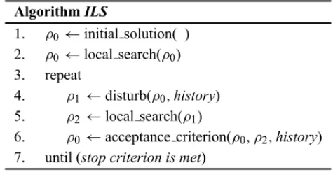
Search method, ILS, is an alternative to prevent that effect. The method is thought to perform a biased sampling of the search space by performing small perturbations in the solution gener-ated by the local search procedure and using this disturbed solution as the starting solution of the next iteration (Lourenc¸oet al., 2003). An ILS approach with the 2-exchange neighborhood is proposed for the QAP by St ¨utzle (2006). The general ILS framework and the ILS algorithm proposed for the QAP are reviewed in the following, since the ILS algorithm proposed by St ¨utzle (2006) is tested in the computational experiments presented in this paper and also the ILS archi-tecture is used in the implementation of the proposed methods. A general framework of the ILS algorithm is presented in Figure 1.
AlgorithmILS
1. ρ0←initial solution( ) 2. ρ0←local search(ρ0) 3. repeat
4. ρ1←disturb(ρ0,history) 5. ρ2←local search(ρ1)
6. ρ0←acceptance criterion(ρ0,ρ2,history) 7. until (stop criterion is met)
Figure 1– General framework of ILS.
An initial solution is generated and a local search is applied to it in steps 1 and 2, respectively. The ILS algorithm may use or not a set to store the history of the search, called history in Figure 1. This set may contain, for example, interesting solutions generated during the search. The history of the search may influence the decisions made in steps 4 and 6. Although history can be considered, in many ILS implementations, the decisions regarding the perturbation of the current solution (step 4) and acceptance criterion (step 6) do not depend on it. The solution generated in the first two steps is disturbed and a local search is applied to the new solution in steps 4 and 5, respectively. In order to re-start the search, an acceptance criterion chooses from which solution the search will be continued. At least, two new decisions, beyond those of the local search method, have to be made in order to use an iterated local search algorithm: the method to disturb solutions and the criteria to accept a solution.
when compared to the other three versions and was implemented in our computational experi-ments for the comparison with the other algorithms. The implementation followed the directions given in the paper it was presented. The local search procedure uses the first pivoting rule and “don’t look bits”. St¨utzle (2006) presents experimental results of the iterated local search algo-rithms for 38 instances withn ranging from 20 to 100. The ILS algorithm is then embedded in an evolutionary algorithm that presents high quality results.
Multi-exchange neighborhoods are natural extensions of the 2-exchange. Ahuja et al. (2007) investigate multi-exchange neighborhoods for the QAP. They definedρ′, ak-exchange neighbor ofρ, as the permutation obtained fromρby a cyclic sequence ofkelements. Given a sequence of locations i1, . . . ,ik, the multi-exchange move corresponds to assign facility ρ(ij)to loca-tionij+1, for all j 6= kand to assign facilityρ(ik)to locationi1. The local search algorithm iteratively examines all cyclic sequences of increasing values for k, where the maximum is a specified parameter. The size of the neighborhood grows exponentially withk, thus this neigh-borhood structure is classified as a Very Large Scale Neighneigh-borhood, for which an exhaustive examination of the whole neighborhood is impracticable in computational terms. With the use of an improvement graph, Ahujaet al. (2007) show that, in average, they can compute the cost of ak-exchange move inO(k). Due to the high processing times needed to the full enumeration scheme the authors established a maximum value for kequals 4. They test multi-start imple-mentations of the proposed neighborhood structure against a multi-start implementation of the 2-exchange neighborhood in 132 test cases of the QAPLIB, with fixed processing times. They show that their neighborhood obtains consistently better results than the multi-start local search with the 2-exchange neighborhood.
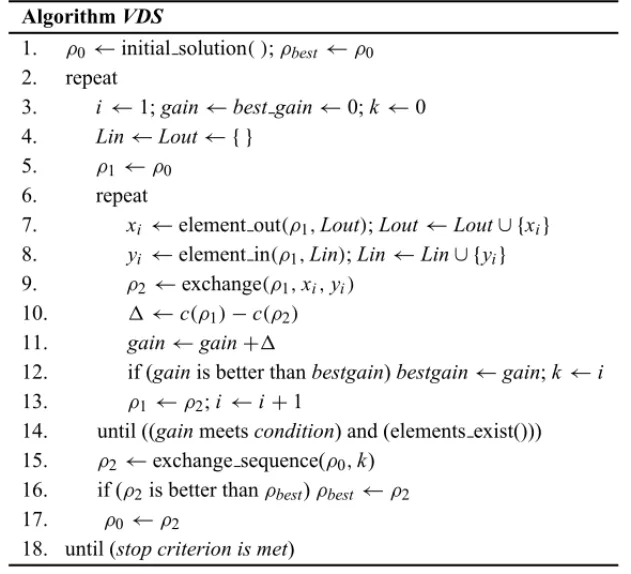
In general, for fixed values, askgrows, the computational effort to deal withk-exchange neigh-borhoods rises rapidly and, usually, the improvement in the quality of solutions does not com-pensate a greater effort. An effective alternative for the fixed size neighborhood structures is presented by Kernighan & Lin (1970) and Lin & Kernighan (1973) for the Partitioning Problem and the Traveling Salesman Problem, respectively. The idea is to perform sequences of moves, such that each move is likely to lead to a better solution instead of testing all moves of a given neighborhood. This method is called Variable Depth Search (VDS). The VDS algorithm exam-ines iteratively, for growing values ofk, whether exchangingkelements may result in a better neighboring solution. A gain function is computed and if it is likely that the previous solution can be improved, then the algorithm tests ifkcan be extended tok+1. When no more gain can be made, the algorithm performs the exchange of thekelements. The general framework of a VDS algorithm is shown in Figure 2.
AlgorithmVDS
1. ρ0←initial solution( );ρbest ←ρ0 2. repeat
3. i ←1;gain←best gain←0;k←0 4. Lin←Lout← { }
5. ρ1←ρ0 6. repeat
7. xi ←element out(ρ1,Lout);Lout←Lout∪ {xi} 8. yi ←element in(ρ1,Lin);Lin←Lin∪ {yi} 9. ρ2←exchange(ρ1,xi,yi)
10. 1←c(ρ1)−c(ρ2) 11. gain←gain+1
12. if (gainis better thanbestgain)bestgain←gain;k←i 13. ρ1←ρ2;i ←i+1
14. until ((gainmeetscondition) and (elements exist())) 15. ρ2←exchange sequence(ρ0,k)
16. if (ρ2is better thanρbest)ρbest ←ρ2 17. ρ0←ρ2
18. until (stop criterion is met)
Figure 2– General framework of VDS.
andLincontain elements that were withdrawn and included in the current solution, respectively. The choice of elementsxi(that is withdrawn) andyi(that is included in the current solution) aims at maximizing the improvement of the current solution within the sequence of moves. Variable ρ1 stores the neighboring solutions found during the VDS iterations. A test is done in step 14 to find out if, given conditions established in advance, the value ingainstill indicates that an improvement exists with the current sequence of moves. The inner loop also finishes if no elements exist to be exchanged due to the restrictions imposed by the lists of prohibited elements what is verified in procedureelement exist( ). In step 15 a new solutionρ2 is generated with the replacement of elementsx1, . . . ,xk by y1, . . . ,yk in solutionρ0. The main loop continues iterating until a given stop criterion is met.
who propose an ejection chain algorithm. Their method builds sequences of exchanges until no promising permutations are likely to exist or until a maximum of n moves. Initially, the best 2-exchange move for each facilityρ(i),i =1, . . . ,n, is identified. Let j be the best location for facilityρ(i), then this facility is assigned to location j. The facility that previously occupied position j is said to be ejected and has to be assigned to other location. The method prohibits elements to be moved twice. Thus the sequence can grow until allnfacilities are moved. Each element of the move sequence corresponds to one local search step in a QAP instance ofq ele-ments, whereqvaries fromnto 1.
4.2 Experiments Comparing Local Search Algorithms
The algorithms by Liet al. (1994) and Regoet al. (2006) were implemented under an iterated local search framework and are named IT-LPR and IT-EC, respectively. The solution generated by the algorithm presented by Regoet al.(2006) is not guaranteed to be a local optimum for the 2-exchange neighborhood. Therefore, a final 2-exchange local search step was included at the end of the iterated local search iterations. Preliminary experiments showed that this modifica-tion improved significantly the performance of this algorithm.
The VDS algorithms are compared to the LSMC (St ¨utzle, 2006) and to the VLSN (Ahujaet al., 2007). For the experiments performed in this paper, we tested two methods to update the “don’t look bits” in the LSMC. The first method followed the directions given in the reference paper by St¨utzle (2006) where only the “don’t look bits” of exchanged elements are reset to 0. In the second method all “don’t look bits” are reset to 0 after a solution is disturbed. The results of the experimentation made to compare these methods showed that the first method produces worse solutions than the second method for the majority of the tested instances. Thus, for compari-son purposes, the best result found for each instance by one of these two versions is reported for LSMC.
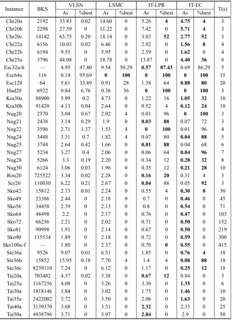
The results listed in columns related to the VLSN were reported by Ahuja et al. (2007) who used an IBM RS6000 platform (333 MHz). Their stopping criterion was 1 hour for problems with n ≥ 40 and 2 hours for problems greater than 40. The stop condition for LSMC, IT-LPR and IT-EC is the maximum processing time (in seconds) shown in the last column of Tables 1 and 2. These tables present the results for symmetric and asymmetric QAPLIB in-stances, respectively. The name of the instance is presented in the first column followed by the best known solution in the second column. Columns Avand %best present, respectively, the average percent deviation from the best known solution and the percentage of best known solutions obtained in 25 independent executions. The results obtained for instances Esc32x, Sko100x and Bur26x are grouped. In these cases the best known solution is not presented in the correspondent column. The best result obtained for each instance by one of the compared algorithms is bold.
Table 1– Comparing local search methods and variants on symmetric QAP instances.
Instance BKS VLSN LSMC IT-LPR IT-EC T(s)
Av %best Av %best Av %best Av %best
Chr20a 2192 33.83 0.02 14.60 0 5.26 4 4.75 4 3
Chr20b 2298 27.59 0 11.22 0 7.42 0 5.71 4 3
Chr20c 14142 63.75 0.20 18.14 0 3.03 52 2.77 52 3
Chr22a 6156 10.03 0.02 6.46 0 2.92 0 1.56 8 4
Chr22b 6194 9.55 0 5.95 0 2.59 0 1.62 0 4
Chr25a 3796 44.08 0 18.78 0 13.87 0 4.40 36 6
Esc32a-h — 4.95 47.80 9.54 50.29 0.57 87.43 0.69 86.29 5
Esc64a 116 0.14 95.69 0 100 0 100 0 100 15
Esc128 64 5.61 33.89 0.91 28 1.38 64 0.88 80 20
Had20 6922 0.84 6.76 0.36 36 0 100 0 100 3
Kra30a 88900 5.99 0.2 4.73 0 1.22 16 1.05 32 10
Kra30b 91420 4.13 0.04 2.64 0 0.52 4 0.12 24 10
Nug20 2570 3.04 0.67 2.02 4 0.01 96 0 100 3
Nug21 2438 3.14 0.29 1.9 0 0.03 88 0.07 72 3
Nug22 3596 2.71 1.37 1.53 4 0 100 0.01 96 4
Nug24 3488 3.31 0.7 1.82 4 0.07 80 0.04 88 5
Nug25 3744 2.64 0.42 1.66 0 0.01 88 0.04 68 6
Nug27 5234 3.27 0.4 2.06 0 0.06 64 0.04 96 7
Nug28 5266 3.3 0.19 2.20 0 0.34 12 0.28 32 8
Nug30 6124 3.06 0.03 1.96 0 0.35 12 0.21 28 10
Rou20 725522 3.34 0.02 2.28 0 0.16 20 0.31 4 3
Scr20 110030 6.22 0.21 2.67 0 0.04 88 0.05 92 3
Sko42 15812 2.73 0.01 2.24 0 0.55 4 0.30 8 30
Sko49 23386 2.44 0 2.18 0 0.7 0 0.46 0 45
Sko56 34458 2.39 0 2.13 0 0.8 0 0.54 0 71
Sko64 48498 2.2 0 2.17 0 0.76 0 0.47 0 103
Sko72 66256 2.21 0 2.02 0 0.71 0 0.50 0 152
Sko81 90998 1.91 0 2.14 0 0.67 0 0.50 0 219
Sko90 115534 1.89 0 2.18 0 0.72 0 0.59 0 300
Sko100a-f — 1.80 0 2.37 0 0.70 0 0.55 0 415
Ste36a 9526 9.07 0.01 6.51 0 1.85 0 0.76 4 18
Ste36b 15852 15.95 0.18 7.70 4 1.4 4 0.08 88 18
Ste36c 8239110 7.24 0 6.12 0 1.17 0 0.25 12 18
Tai20a 703482 4.37 0.02 3.38 0 0.67 12 0.84 0 3
Tai25a 1167256 4.08 0 3.26 0 3.30 0 1.35 0 6
Tai30a 1818146 3.84 0 3.02 0 1.75 0 1.46 0 10
Tai35a 2422002 3.72 0 3.50 0 2.06 0 1.63 0 20
Tai40a 3139370 3.68 0 3.51 0 2.32 0 2.35 0 25
Table 1(continuation) – Comparing local search methods and variants on symmetric QAP instances.
Instance BKS VLSN LSMC IT-LPR IT-EC T(s)
Av %best Av %best Av %best Av %best
Tai60a 7205962 3.54 0 3.83 0 2.87 0 3.03 0 89
Tai80a 13511780 2.78 0 3.32 0 2.74 0 2.58 0 223
Tai100a 21052466 2.49 0 3.16 0 2.57 0 2.71 0 1000
Tho30 149936 3.72 0.03 3.34 0 0.43 16 0.3 20 10
Tho40 240516 3.70 0 2.97 0 1.01 0 0.52 0 25
Tho150 8133398 2.12 0 3.64 0 0.79 0 0.68 0 1000
Wil50 48816 1.37 0 1.07 0 0.20 0 0.11 0 120
Wil100 273038 0.95 0 3.12 0 0.35 0 0.25 0 1000
Table 2– Results for asymmetric instances.
Instance BKS VLSN LSMC IT-LPR IT-EC T(s)
Av %best Av %best Av %best Av %best
Bur26a-h —– 0.27 1.99 0.26 0.13 0.08 0 0.00 85.50 15
Lipa20a 3683 2.52 1.37 1.93 12 0 100 0 100 3
Lipa30a 13178 1.83 0.24 1.77 0 1.01 24 0.56 60 4
Lipa40a 31538 1.36 0.01 1.23 0 1.13 0 0.80 28 25
Lipa50a 62093 1.17 0 1.14 0 1.02 0 0.93 8 50
Lipa60a 107218 0.99 0 0.99 0 0.90 0 0.90 0 89
Lipa70a 169755 0.86 0 0.88 0 0.80 0 0.80 0 150
Lipa80a 253195 0.75 0 0.77 0 0.71 0 0.72 0 225
Lipa90a 360630 0.69 0 0.73 0 0.67 0 0.67 0 300
Lipa20b 27076 12.66 12.94 9.67 32 0 100 0 100 3
Lipa30b 151426 14.96 7.34 14.05 12 0 100 1.80 88 4
Lipa40b 476581 16.9 5.8 17.20 0 0.66 96 1.39 92 5
Lipa50b 1210244 17.52 2.33 18.90 0 8.26 52 5.61 68 10
Lipa60b 2520135 19.22 0.42 20.66 0 16.66 12 17.57 8 17
Lipa70b 4603200 19.94 0.53 21.07 0 16.65 16 18.32 8 30
Lipa80b 7763962 20.92 0.08 21.74 0 19.94 4 20.92 0 45
Lipa90b 12490441 — — 26.61 0 19.43 8 20.38 4 60
Tai20b 122455319 14.22 6.3 0.79 28 0 100 0 100 3
Tai25b 344355646 12.1 0.59 4.66 0 0.07 48 0 100 15
Tai30b 637117113 9.06 0.13 2.60 0 0.20 4 0 100 25
Tai35b 283315445 6.47 0.03 4.86 0 0.25 4 0.09 60 39
Tai40b 637250948 8.29 0.24 6.26 0 0.05 12 0.00 96 59
Tai50b 458821517 5.73 0 4.15 0 0.27 0 0.27 24 116
Tai60b 608215054 6.16 0 4.80 0 0.30 0 0.54 4 211
Tai80b 818415043 5.27 0 3.84 0 1.09 0 0.92 0 500
Tai100b 1185996137 4.43 0 2.05 0 0.64 0 0.46 0 1000
results in Table 1 show that the two VDS algorithms present, in general, the best performance for the 58 symmetric instances of the computational experiment. The IT-LPR presents the best average results on 18 instances. The IT-EC presents the overall best performance regarding qual-ity of solution. It presents 46 best average results including instances Esc32c, Esc32d, Esc32e, Esc32g and the whole Sko100 set. The number of best known solutions produced by the two VDS algorithms is similar with some advantage for the IT-EC. The average concerning the 58 symmetric instances and the 25 independent executions are 4.02, 4.90, 23.65 and 28.39 for the VLSN, LSMC, IT-LPR and IT-EC, respectively.
The Kruskal-Wallis’ statistical test was applied to determine if significant differences exist be-tween the results presented by the three ILS algorithms. The VLSN could not be tested, once the results for each instance are not available. The results of the statistical test considering signif-icance level 0.05 showed that the null hypothesis (samples come from identical populations) cannot be rejected only for instances Esc32c, Esc32e, Esc32g, Esc64a and Esc128, indicat-ing that for the other 53 instances the results produced by at least one algorithm were signif-icantly different from the other two. In all cases the test indicated that the LSMC performed significantly worse than the other algorithms. The Mann-Whitney U-test was applied to the re-sults of the two VDS algorithms. With significance level 0.05, the test showed that the IT-EC produced significantly superior results on instances Chr22a, Chr22b, Chr25a, Kra30b, Nug27, Nug28, Tai25a, Tai35a, Sko42, Sko49, Sko56, Sko64, Sko72, Sko81, Sko90, Sko100a-f, Ste36a-c, Tho30, Tho40, Tho150, Wil50 and Wil100. Significant better results were presented by the IT-LPR on instances: Rou20, Tai50a, Tai60a, Tai80a and Tai100a.
In order to apply the test for proportions comparison (Taillardet al., 2008) it is necessary to define “success” In this paper, one algorithm is considered successful on one instance when compared to other, if the former produces a better average value than the latter. With significance level 0.01, the statistical test showed that the IT-EC was the best approach when compared to each of the other three algorithms. The VLSN performed conclusively worse than the others. The comparison between the IT-LPR and to the LSMC showed that that the former outperformed the latter.
The test for proportions comparison with significance level 0.01 showed that the two VDS algo-rithms outperform the VLSN and the LSMC. The null hypothesis cannot be rejected (even with significance level 0.05) in the comparison between VLSN and LSMC. The test also pointed out a significant better result of the IT-EC over the IT-LPR.
5 GUIDING VDS WITH THE COSTS OF EDGE ASSIGNMENTS
In terms of Graph Theory, each parcel of equation 1 corresponds to the cost of an assignment of two edges of complete graphs of ordern. From this viewpoint, the objective function seeks at minimizing the sum of products of edge weights. The problem of assigning edges is solved in polynomial time, but only few assignments of edges, regarding the total number of such as-signments, lead to feasible solutions concerning the assignment of vertices whenn >3 (Rangel & Abreu, 2007). Nevertheless, the costs of the edges assignments can be used to guide the search indicating goodcandidates to be exchanged. In this sense, the edges are thought as the exchanging elements, taking due care to maintain feasibility of the solutions produced during the search. Given a solution, ρ, the flow edge ef with terminal verticesρ(i)and ρ(j) and the location edge ed with terminal vertices i and j, the assignment of edges is represented by(ef,ed).
Consider that edge ef is assigned toed, the assignment ofef to a new locationed′ implies in freeing the edgee′f, previously assigned toe′d. Therefore, the basic idea consists in, iteratively, canceling an edge assignment and to re-assign the freed flow edge to another distance edge.
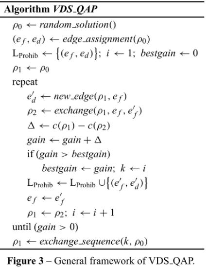
In this paper, two alternatives are considered for the new assignment. In the first alternative, the assignment of one terminal vertex ofef is undone and the assignment of the other terminal vertex remains fixed. In the other alternative both assignments of the terminal vertices of edge ef are undone. In both cases, the freed vertex(vertices) is(are) assigned to a new location(s). This new assignment induces a new solution,ρ1. The difference between the costs of the origi-nal solution,ρ, and the solution induced by the basic move,ρ1, is calculated and the gain func-tion is updated. The first and the second alternatives lead to one and two algorithmic versions, respectively. The general framework of the variable-depth search based on the first alternative is presented in algorithm VDS QAP.
After the initial solution,ρ0, is generated, the first assignment of edges to be undone is chosen in procedureedge assignment( ). A list of prohibited moves, LProhib, stores the pair of edges
AlgorithmVDS QAP
ρ0←random solution() (ef,ed)←edge assignment(ρ0) LProhib←
(ef,ed) ; i←1; bestgain←0
ρ1←ρ0 repeat
e′d←new edge(ρ1,ef)
ρ2←exchange(ρ1,ef,e′f)
1←c(ρ1)−c(ρ2) gain←gain+1 if (gain>bestgain)
bestgain←gain; k←i LProhib←LProhib∪
(e′f,e′d) ef ←e′f
ρ1←ρ2; i←i+1 until (gain>0)
ρ1←exchange sequence(k, ρ0)
Figure 3– General framework of VDS QAP.
in LProhib, then the new pair is added to it. Otherwise, the new element replaces the “oldest”
element of LProhib. The main loop iterates while positive gains exist (variable gain is greater than
0). Alternatively a stopping criterion can also consider a maximum number of iterations of the main loop. Finally, the initial solution,ρ0, is updated with the best sequence of edges exchange in procedureexchange sequence( ).
Two important decisions to be made when implementing VDS QAP are: to define how many and which assignments are canceled at each iteration step and to define how the new locations for the freed edges are chosen. A number of alternatives exist for these and other implementa-tion issues. Depending on the decisions made by the developer, algorithms with wide varying behaviors are expected to be created. In the next two sections, three algorithmic versions are presented where the details concerning those decisions are explained.
In the algorithms presented in the next sections, the choice of the first edge assignment that is undone is based on the cost of the assignments of each pair of edges in the initial solution. Given a solution,ρ, the weight of the assignment(ef,ed)of edge ef with terminal verticesρ(i)and
ρ(j)to edgeed with terminal verticesi and j is given byw(ef,ed)= fρ(i)ρ(j)di j. In order to select the first pair,(ef,ed), a restricted list of candidates is built with thelsize% pairs with the greatest weights. One element of that list is randomly chosen with a probability that is directly proportional to the weight of the correspondent assignment.
It was observed that the best results were obtained with 10 or 30, with the latter value yielding slightly better results than the former.
The sequence of movements is terminated ifgain≤0. In the implementations reported here an additional stopping criterion was added to establish a maximum number of iterations being twice the size of LProhibwithout the improvement of the best solution found up to the current iteration.
The size of LProhibwas set to 150 after preliminary experiments.
5.1 One Terminal Vertex is set Free – VDS1
In the first variant of the proposed algorithm, denoted as VDS1, only one terminal vertex of edge ef is set free. Thus, it is necessary to decide which terminal vertex assignment remains fixed and which is undone. It corresponds to choose which location of edgeedbecomes unoccupied. This decision is made simultaneously with the choice of the new location for the free facility. Both terminal vertices of edgeef are tested.
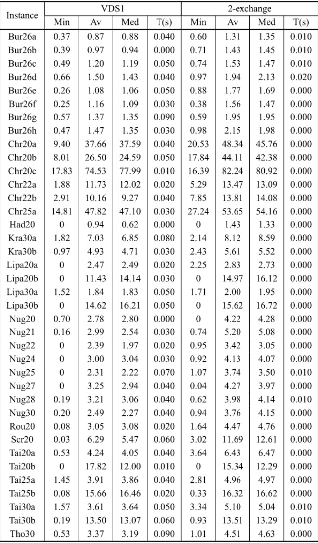
In a first experiment to examine the potential of the variant VDS1 in relation to the 2-exchange neighborhood, 100 random re-starts of each method were applied to all QAPLIB instances with n ranging from 20 to 30. In this experiment, each released vertex was tested in all locations not prohibited for it. The minimal, average and median solution reached by each method were computed, as well as the average processing time. The results are shown in Table 3 where the values of the minimal, average and median solutions are reported in columnsMin,AvandMed, respectively. The average processing time in seconds is exhibited in columnT.
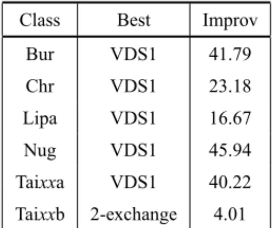
The results presented in Table 3 show that the minimal values obtained by VDS1 are better than the ones produced by the 2-exchange on 32 of the 38 instances, there are 4 ties and the latter method finds 2 minimal values better than the former. The proposed method also finds the best average solutions on 36 instances. All median values produced by the VDS1 are lower than the median values obtained with the other method. A summary of the improvements in average solutions obtained by VDS1 over the other algorithm per instance class is shown in Table 4. The values exhibited in Table 4 were calculated on classes with at least three instances. Columns Class,BestandImprovementshow, respectively, the class name, which algorithm produced the best average value and the improvement of the average solution over the other algorithm.
Table 4 shows that the 2-exchange local search exhibits better results on Taixxb class, where an improvement of 4.01% is obtained. The proposed approach outperforms the 2-exchange algo-rithm on the remaining instances with the lowest improvement being 16.67% on class Lipa.
Table 3– Results of 100 random starts of methods VDS1 and 2-exchange local search.
Instance VDS1 2-exchange
Min Av Med T(s) Min Av Med T(s)
Bur26a 0.37 0.87 0.88 0.040 0.60 1.31 1.35 0.010
Bur26b 0.39 0.97 0.94 0.000 0.71 1.43 1.45 0.010
Bur26c 0.49 1.20 1.19 0.050 0.74 1.53 1.47 0.010
Bur26d 0.66 1.50 1.43 0.040 0.97 1.94 2.13 0.020
Bur26e 0.26 1.08 1.06 0.050 0.88 1.77 1.69 0.000
Bur26f 0.25 1.16 1.09 0.030 0.38 1.56 1.47 0.000
Bur26g 0.57 1.37 1.35 0.090 0.59 1.95 1.95 0.000
Bur26h 0.47 1.47 1.35 0.030 0.98 2.15 1.98 0.000
Chr20a 9.40 37.66 37.59 0.040 20.53 48.34 45.76 0.000 Chr20b 8.01 26.50 24.59 0.050 17.84 44.11 42.38 0.000 Chr20c 17.83 74.53 77.99 0.010 16.39 82.24 80.92 0.000 Chr22a 1.88 11.73 12.02 0.020 5.29 13.47 13.09 0.000 Chr22b 2.91 10.16 9.27 0.040 7.85 13.81 14.08 0.000 Chr25a 14.81 47.82 47.10 0.030 27.24 53.65 54.16 0.000
Had20 0 0.94 0.62 0.000 0 1.43 1.33 0.000
Kra30a 1.82 7.03 6.85 0.080 2.14 8.12 8.59 0.000
Kra30b 0.97 4.93 4.71 0.030 2.43 5.61 5.52 0.000
Lipa20a 0 2.47 2.49 0.020 2.25 2.83 2.73 0.000
Lipa20b 0 11.43 14.14 0.030 0 14.97 16.12 0.000
Lipa30a 1.52 1.84 1.83 0.050 1.71 2.00 1.95 0.000
Lipa30b 0 14.62 16.21 0.050 0 15.62 16.72 0.000
Nug20 0.70 2.78 2.80 0.000 0 4.22 4.28 0.000
Nug21 0.16 2.99 2.54 0.030 0.74 5.20 5.08 0.000
Nug22 0 2.39 1.97 0.020 0.95 3.42 3.05 0.000
Nug24 0 3.00 3.04 0.030 0.92 4.13 4.07 0.000
Nug25 0 2.31 2.22 0.070 1.07 3.74 3.50 0.010
Nug27 0 3.25 2.94 0.040 0.04 4.27 3.97 0.000
Nug28 0.19 3.21 3.06 0.040 0.62 3.98 4.14 0.010
Nug30 0.20 2.49 2.27 0.040 0.94 3.76 4.15 0.000
Rou20 0.08 3.05 3.08 0.020 1.64 4.47 4.76 0.000
Scr20 0.03 6.29 5.47 0.060 3.02 11.69 12.61 0.000
Tai20a 0.53 4.24 4.05 0.040 3.64 6.43 6.47 0.000
Tai20b 0 17.82 12.00 0.010 0 15.34 12.29 0.000
Tai25a 1.45 3.91 3.86 0.040 2.81 4.96 4.97 0.000
Tai25b 0.08 15.66 16.46 0.020 0.33 16.32 16.62 0.000
Tai30a 1.57 3.61 3.64 0.050 3.34 5.10 5.04 0.010
Tai30b 0.19 13.50 13.07 0.060 0.93 13.51 13.29 0.010
Table 4– Improvements on average solutions per instance class.
Class Best Improv
Bur VDS1 41.79
Chr VDS1 23.18
Lipa VDS1 16.67
Nug VDS1 45.94
Taixxa VDS1 40.22
Taixxb 2-exchange 4.01
of the 38 instances only. It means that on the majority of instances, 28 of 38, the statistical test did not indicate significant differences regarding computational times.
In the ILS version of VDS1, two matrices are used to establish a preference order among the localities to which a free facility can be assigned. In a pre-processing phase, two matricesn×n−1 of ranks,RF andRD, are built from FandD, respectively. In order to generate these matrices, a list is created for each facility(location) that contains the remaining facilities(locations) in non-decreasing(non-increasing) order of flow(distance). ElementRF[p][q]is the position of facility
q in the list built for facility p. Element RD[p][q]is the locality that is in theq-th position of the list correspondent to location p.
Letρ(i)andρ(j)be the free and the fixed vertices, respectively, of edgeef. A list of possible locations forρ(i),Lposs, is built with basis on RD and element RF[ρ(j)][ρ(i)]. Since j is the occupied location, the first candidate as the new location of facilityρ(i)to be included inLposs is the element in position RF[ρ(j)][ρ(i)]of the list of locations corresponding to j, that is, element RD[j][RF[ρ(j)][ρ(i)]]. The other elements ofLpossare RD[j][RF[ρ(j)][ρ(i)+1],
RD[j][RF[ρ(j)][ρ(i)−1], . . . ,RD[j][RF[ρ(j)][ρ(i)+k], RD[j][RF[ρ(j)][ρ(i)−k]. If it is the case thatρ(i)−k =0 andρ(i)+k <n−1 orρ(i)] −k > 0 andρ(i)+k =n −1, Lpossis completed with elementsRD[j][RF[ρ(j)][ρ(i)+k+1], . . . ,RD[j][RF[ρ(j)][n−1], or
RD[j][RF[ρ(j)][ρ(i)−k], . . . ,RD[j][RF[ρ(j)][1], respectively. Therefore,Lpossis mounted with the locations with best chance of being a good location forρ(i)according to the values of the corresponding edges. The algorithm seeks the new location forρ(i), analyzing the exchange ofρ(i)andρ(h),h being the current location examined of listLposs. In the algorithm described in this paper, a first improvement rule was used. Let bestloc be the best location found for ρ(i). Then a new solutionρ1with costc(ρ1)is induced by the interchange of verticesρ(i)and ρ(bestloc). The same analysis is done for vertexρ(j)resulting in solution ρ2with costc(ρ2). The assignment that induces the solution with the lowest cost amongρ1andρ2is assumed as the exchange move.
5.2 Two Terminal Vertexes are Set Free – VDS2
to be time consuming in this case, once two vertices need to be re-located. Thus, in the VDS2 versions, the choice of the distance edgee′
dto whichef is assigned has a random element. Two versions of VDS2 are investigated. These variants do not use the list of forbidden movements. This occurs because the probability of undoing previous movements is very small due to the randomness on the choice of the new assignments.
The first version, named VDS2A, in order to definee′
d, one location is selected at random. Let us consider that edgeedhas no facilities assigned to its terminal vertices, since the current facilities will be removed. One facility,fac1, is chosen at random with equal probability to be assigned to one terminal vertex ofed. Letiand jbe the terminal vertices of edge ed and suppose thatfac1 is assigned to locationi. If j is thek-th element in the list of vertexi, regarding the distances betweeni and the other locations, then the candidate facilities to be assigned to the second free location are close to the k-th element of the corresponding list of fac1. In the algorithm implemented in this paper, the facilities in positionsk±ain the list offac1are the candidates to be the facility that will be assigned to location j. In this version, one of these facilities is selected at random with uniform probability. Preliminary tests evaluated values 0, 1 and 2 for variablea. The experiments showed that the results witha =0 were inferior to botha =1 anda =2. A small advantage was observed fora =2 with no significant difference in processing time. Once the two new facilities are chosen, the algorithm determines the best assignment among the two pair of facilities, the ones that left the locations and the new ones.
In the second VDS2 version, VDS2R, ed′ is selected at random among the possible distance edges.
The absence of the best improvement criterion employed in VDS1 reflects on the quality of solu-tions, but a gain regarding the processing times is obtained. Like in the IT-EC, to guarantee that the solution produced by each algorithm is a local optimum for the 2-exchange neighborhood, a final 2-exchange local search step was included at the end of each ILS iteration.
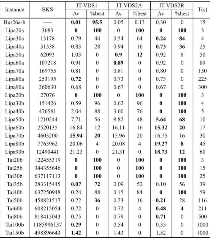
Tables 5 and 6 present the results of the computational experiments regarding symmetric and asymmetric QAPLIB instances for the iterated local search versions of the three proposed VDS algorithms. The Kruskal-Wallis’ statistical test with significance level 0.05 was applied to de-termine if differences exist between the results presented by the three new algorithms.
Table 5– Edge assignment based VDS for QAPLIB symmetric instances.
Instance BKS IT-VDS1 IT-VDS2A IT-VDS2R T(s)
Av %best Av %best Av %best
Chr20a 2192 3.38 28 2.62 8 3.05 16 3
Chr20b 2298 5.52 8 6.44 0 5.36 0 3
Chr20c 14142 1.76 68 2.43 76 1.49 76 3
Chr22a 6156 1.29 8 1.06 32 1.17 20 4
Chr22b 6194 1.72 0 1.82 4 1.60 20 4
Chr25a 3796 3.73 28 5.81 32 5.37 12 6
Esc32a-h — 0.85 83.43 1.32 82.29 1.16 83.43 5
Esc64a 116 0 100 0.21 92 0 100 15
Esc128 64 0.88 76 4.25 32 2.63 60 20
Had20 6922 0 100 0 100 0 100 3
Kra30a 88900 1.18 20 1.28 28 1.10 24 10
Kra30b 91420 0.13 32 0.21 24 0.21 24 10
Nug20 2570 0 100 0 100 0 100 3
Nug21 2438 0.09 60 0.02 88 0.03 84 3
Nug22 3596 0 100 0 100 0 100 4
Nug24 3488 0.13 68 0.04 92 0.01 96 5
Nug25 3744 0.01 80 0.02 76 0.02 80 6
Nug27 5234 0 100 0 100 0 100 7
Nug28 5166 0.17 48 0.26 48 0.22 52 8
Nug30 6124 0.20 20 0.28 8 0.13 40 10
Rou20 725522 0.22 4 0.20 4 0.20 16 3
Scr20 110030 0.05 88 0.14 72 0.01 96 3
Sko42 15812 0.24 20 0.37 4 0.27 4 30
Sko49 23386 0.41 0 0.37 0 0.40 0 45
Sko56 34458 0.48 0 0.56 0 0.42 0 71
Sko64 48498 0.5 0 0.47 0 0.49 0 103
Sko72 66256 0.49 0 0.56 0 0.51 0 152
Sko81 90998 0.47 0 0.47 0 0.44 0 219
Sko90 115534 0.61 0 0.58 0 0.55 0 300
Sko100a-f — 0.54 0 0.58 0 0.55 0 415
Ste36a 9526 0.56 12 0.86 8 0.52 20 18
Ste36b 15852 0.01 96 0.11 88 0.01 96 18
Ste36c 8239110 0.22 12 0.31 32 0.32 12 18
Tai20a 703482 0.72 2 0.52 3 0.60 3 3
Tai25a 1167256 1.29 1 1.30 0 1.47 0 6
Tai30a 1818146 1.52 0 1.79 0 1.55 0 10
Tai35a 2422002 1.76 0 1.90 0 1.73 0 20
Tai40a 3139370 2.22 0 2.45 0 2.73 0 25
Table 5(continuation) – Edge assignment based VDS for QAPLIB symmetric instances.
Instance BKS IT-VDS1 IT-VDS2A IT-VDS2R T(s)
Av %best Av %best Av %best
Tai60a 7205962 2.95 0 3.05 0 3.10 0 89
Tai80a 13511780 2.48 0 2.95 0 2.89 0 223
Tai100a 21052466 2.77 0 2.69 0 2.73 0 1000
Tho30 149936 0.21 40 0.24 28 0.27 32 10
Tho40 240516 0.65 0 0.62 0 0.45 0 25
Tho150 8133398 0.66 0 0.77 0 0.75 0 1000
Wil50 48816 0.12 4 0.11 0 0.09 0 120
Wil100 273038 0.26 0 0.25 0 0.25 0 1000
Table 6– Edge assignment based VDS for QAPLIB asymmetric instances.
Instance BKS IT-VDS1 IT-VDS2A IT-VDS2R T(s)
Av %best Av %best Av %best
Bur26a-h —– 0.01 95.5 0.05 0.13 0.30 0 15
Lipa20a 3683 0 100 0 100 0 100 3
Lipa30a 13178 0.79 44 0.54 64 0.24 84 4
Lipa40a 31538 0.83 28 0.94 16 0.73 36 25
Lipa50a 62093 1.03 0 0.9 12 0.92 8 50
Lipa60a 107218 0.91 0 0.89 0 0.92 0 89
Lipa70a 169755 0.81 0 0.81 0 0.80 0 150
Lipa80a 253195 0.72 0 0.73 0 0.73 0 225
Lipa90a 360630 0.68 0 0.67 0 0.67 0 300
Lipa20b 27076 0 100 0 100 0 100 3
Lipa30b 151426 0.59 96 0.62 96 0 100 4
Lipa40b 476581 2.04 88 3.60 76 0 100 5
Lipa50b 1210244 7.71 56 8.82 48 5.64 68 10
Lipa60b 2520135 16.84 12 16.11 16 15.32 20 17
Lipa70b 4603200 15.94 20 15.96 20 16.75 16 30
Lipa80b 7763962 20.06 4 20.08 4 19.27 8 45
Lipa90b 12490441 21.23 0 21.31 0 18.73 12 60
Tai20b 122455319 0 100 0 100 0 100 3
Tai25b 344355646 0 100 0 100 0 100 15
Tai30b 637117113 0 100 0 100 0 100 25
Tai35b 283315445 0.07 72 0.09 52 0.10 56 39
Tai40b 637250948 0.24 88 0.15 84 0 100 59
Tai50b 458821517 0.22 36 0.23 16 0.21 28 116
Tai60b 608215054 0.72 0 0.72 4 0.48 4 211
Tai80b 818415043 0.75 0 0.79 0 0.71 0 500
Tai100b 1185996137 0.29 0 0.54 0 0.35 0 1000
The test for proportions comparison with significance level 0.05 shows that, except for the pair IT-VDS1 and IT-VDS2R, significant differences do exist among the other pairs of algorithms. Considering the averages presented in Tables 1 and 5, that test also shows that the IT-LPR presents significant worse results than the three proposed VDS algorithms in the symmetric QAPLIB instances. IT-VDS2A is outperformed by IT-VDS1, IT-VDS2R and IT-EC. The algo-rithms ITVDS1 and ITVDS2R present better results than the IT-EC. The algorithm IT-VDS1 shows a particular good performance on instances Taixxa where the algorithm presents the best results on six of the nine instances. The algorithms IT-VDS2R and IT-VDS2A present 22 and 13 best average results and 13 and 11 best percentages of the best known solution, respectively. Considering the 25 independent executions of each algorithm for each instance of the experi-ment, the algorithm ITVDS2R obtains, in average, 31.12 % of the best known solutions, fol-lowed by IT-VDS1, 29.92% and IT-VDS2A, 28.90%. These three results are better than the ones presented by algorithms IT-LPR and IT-EC.
Considering the average values presented in Table 6, the test for proportions comparison with significance level 0.05 shows that, the algorithm IT-VDS2R presents significantly better results than the other VDS algorithms on the set of asymmetric instances. The test also points out the best performance of VDS2R over LPR and EC and that the latter outperforms the IT-VDS1. A significant difference is also found in favor of IT-VDS1 against IT-VDS2A. With the specified significance level, it is not possible to point out differences between the other results.
The results concerning the number of best known solutions of the asymmetric instances obtained by the proposed algorithms show that, in average, the algorithm ITVDS2R obtains the best per-formance with 42.22% of the best known solutions, followed by IT-VDS1 with 42.20%, IT-EC with 41.98%, IT-VDS2A with 38.77% and IT-LPR with 25.19%.
5.3 Comparison of the proposed VDS heuristics with an exact algorithm
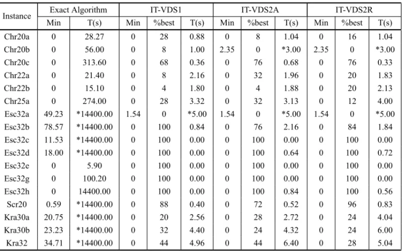
Table 7– Comparison with the results of an exact algorithm.
Instance Exact Algorithm IT-VDS1 IT-VDS2A IT-VDS2R
Min T(s) Min %best T(s) Min %best T(s) Min %best T(s)
Chr20a 0 28.27 0 28 0.88 0 8 1.04 0 16 1.04
Chr20b 0 56.00 0 8 1.00 2.35 0 *3.00 2.35 0 *3.00
Chr20c 0 313.60 0 68 0.36 0 76 0.68 0 76 0.33
Chr22a 0 21.40 0 8 2.16 0 32 1.96 0 20 1.83
Chr22b 0 15.10 0 4 1.80 0 4 1.88 0 20 2.13
Chr25a 0 274.00 0 28 3.32 0 32 3.13 0 12 4.00
Esc32a 49.23 *14400.00 1.54 0 *5.00 1.54 0 *5.00 1.54 0 *5.00
Esc32b 78.57 *14400.00 0 100 0.84 0 76 2.16 0 84 1.84
Esc32c 11.53 *14400.00 0 100 0.00 0 100 0.00 0 100 0.00
Esc32d 18.00 *14400.00 0 100 0.00 0 100 0.64 0 100 0.72
Esc32e 0 5.90 0 100 0.00 0 100 0.00 0 100 0.00
Esc32g 0 100.20 0 100 0.00 0 100 0.00 0 100 0.00
Esc32h 0 14400.00 0 100 0.00 0 100 0.84 0 100 0.56
Scr20 0.59 *14400.00 0 88 0.40 0 72 0.52 0 96 0.83
Kra30a 20.75 *14400.00 0 20 2.56 0 28 2.72 0 24 4.04
Kra30b 23.23 *14400.00 0 32 4.40 0 24 4.32 0 24 6.00
Kra32 34.71 *14400.00 0 44 4.96 0 44 6.40 0 28 5.04
The two ITVDS2 algorithms did not find the optimal solution of the Chr20b instance and no algorithm found the optimal solution of Esc32a instance. The results produced by the exact algorithm on Chr instances are very effective, as shown in Table 7. However on the remain-ing instances, the heuristic algorithms are always preferable to the exact algorithm. Even on the Esc32e instance, where the exact algorithm takes only 5.9s to solve it, the heuristic algo-rithms take, in average, less than 0.01s to find the optimal solution and find the optimum in all executions. The exact algorithm cannot find the optimal solution of eight instances. From those instances, the heuristic algorithm misses the optimum only on instance Esc32a, yet the differ-ence to the optimal value is much smaller as well as the processing time. Another point to consider is that the heuristic algorithms find optimal solutions on instances larger than those considered by the exact algorithms currently proposed for the QAP.
5.4 Testing with Drexxinstances
Instances withn between 15 and 72 were tested. Table 8 shows averages and percentage of optimal solutions obtained by each algorithm. The maximum processing times in seconds are presented in columnT(s).
Table 8– Results for Drexx instances.
Id BKS
IT-EC IT-LPR IT-VDS1 IT-VDS2A IT-VDS2R
T(s)
Av % Av % Av % Av % Av %
best best best best best
Dre15 306 0 100 381.83 0 0 100 0 100 0 100 15
Dre18 332 0 100 414.65 0 0 100 0 100 0 100 18
Dre21 356 8.18 68 428.54 0 4.36 80 5.39 76 4.97 76 21
Dre24 396 23.23 16 443.76 0 21.41 16 20.60 24 24.67 4 24
Dre28 476 26.74 12 450.72 0 30.24 0 26.32 16 29.03 8 28
Dre30 508 40.39 0 448.71 0 38.25 0 44.83 0 45.98 0 30
Dre42 764 62.39 0 471.19 0 67.33 0 67.52 0 69.46 0 42
Dre56 1086 82.42 0 470.85 0 89.22 0 88.53 0 90.12 0 56
Dre72 1452 92.70 0 474.42 0 98.37 0 99.11 0 99.24 0 152
favor of IT-EC were found on instances Dre42, 56 and 72 in comparison to the other three al-gorithms. The test for proportions comparison confirms the best performance of IT-EC on Dre instances in comparison to the IT-VDS2R. Evidences of significant differences are not pointed out by the proportions comparison test in pairwise comparisons of the other algorithms.
5.5 Testing with Taixxe instances
Instances with n = 27, 45 and 75 are tested. The maximum processing times given to the algorithms are 10 seconds(n =27), 30 seconds(n =45)and 200 seconds(n =75). Tables 9, 10 and 11 show the results for classesn =27, 45 and 75, respectively. The first column contains the identification of each test case. The second column shows the optimum or the best known solution of each instance. Columns Md show the percent deviation of the median from the optimum or best known solution. Columns %bestshow the percentage of optimal or best known solutions found by each algorithm.
With significance level 0.05, the Kruskal-Wallis’ test pointed out significant differences on the performance of the algorithms for all instances of class 27, where the inferior performance of IT-LPR was identified. Due to this fact, other comparisons were carried on the results obtained only with the other four algorithms. The success for this set of instances is established on the number of best solutions found by each algorithm. With significance level 0.05, the test for proportion comparison showed that IT-EC and IT-VDS1 are outperformed by IT-VDS2R. In general, IT-VDS1 is outperformed by IT-EC and IT-VDS2A, although the hypothesis test does not point out significant differences. IT-VDS2A and IT-EC performs similarly.
Table 9– Results for Tai27e instances.
Id BKS IT-EC IT-LPR IT-VDS1 IT-VDS2A IT-VDS2R
Md %best Md %best Md %best Md %best Md %best
1 2558 0 96 1.17 32 0 84 0 84 0 84
2 2850 0 88 9.02 0 0 72 0 88 0 76
3 3258 0 100 4.79 4 0 88 0 100 0 100
4 2822 0 100 3.54 16 0 100 0 100 0 100
5 3074 0 84 7.61 4 0 92 0 84 0 100
6 2814 0 100 3.62 48 0 96 0 92 0 88
7 3428 0 84 1.98 32 0 88 0 88 0 84
8 2430 0 100 5.69 20 0 96 0 100 0 100
9 2902 0 80 5.31 12 0 68 0 76 0 88
10 2994 0 100 7.82 12 0 96 0 92 0 100
11 2906 0 80 1.38 48 0 72 0 72 0 80
12 3070 0 80 9.45 8 0 88 0 92 0 84
13 2966 0 68 0.27 44 0 76 0 80 0 88
14 3568 0 88 4.34 16 0 96 0 88 0 96
15 2628 0 76 9.09 8 0 80 0 80 0 80
16 3124 0 100 0 60 0 100 0 96 0 100
17 3840 0 80 1.95 20 0 96 0 96 0 92
18 2758 0 76 3.63 28 0 68 0 96 0 68
19 2514 0 80 7.92 0 0 60 0 76 0 88
20 2638 0 60 3.94 24 0 68 0 68 0 80
equals to BKS is obtained by the IT-VDS1, followed by the IT-VDS2A, IT-EC and IT-VDS2R as shown in Table 10. The test for proportions comparison indicated that IT-VDS1 performs better than IT-VDS2R in the Tai45e instances with confidence level 93.38%. The test did not detect significant differences among the performances of the remaining algorithms.
The Kruskal-Wallis’ test pointed out significant differences between the results presented by at least one algorithm on class Tai75e instances. The Mann-Whitney U-test showed that the IT-LPR performed worse than the IT-VDS1 and IT-VDS2R on 13 instances, the IT-EC on 14 instances and the IT-VDS2A on 17 instances. The test for proportions comparison considering the medians also showed significant differences in favor of IT-VDS1, IT-VDS2A, IT-VDS2R and IT-EC against IT-LPR. At significance level 0.05, the test for proportions comparison showed that IT-EC, IT-VDS2R and IT-VDS2A are outperformed by IT-VDS1. The test does not indicate significant differences among the other three algorithms.
Table 10– Results for Tai45e instances.
Id BKS IT-EC IT-LPR IT-VDS1 IT-VDS2A IT-VDS2R
Md %best Md %best Md %best Md %best Md %best
1 6412 7.29 44 10.01 0 0 52 0 52 0 52
2 5734 0 76 14.82 0 0 64 0 68 0 60
3 7438 0.40 48 15.86 0 8.71 32 1.64 36 8.71 36
4 6698 0 52 12.57 0 7.61 44 6.99 32 7.61 28
5 7274 8.33 28 15.04 0 8.33 40 0 32 8.33 52
6 6612 1.75 48 20.75 0 7.56 40 7.56 52 0 28
7 7526 3.96 40 7.28 4 0 60 0 60 0 72
8 6554 0 60 13.7 0 0 56 5.98 32 5.98 44
9 6648 4.51 36 15.4 0 0 68 0 44 4.51 56
10 8286 0 76 8.35 8 0 60 1.71 60 0 44
11 6510 5.87 32 14.1 0 0 52 0 56 0 64
12 7510 0 64 13.36 8 0.27 48 0 52 0 52
13 6120 7.91 48 11.99 4 8.50 44 4.34 44 1.41 40
14 6854 0 72 18.76 4 0 72 0.09 84 0 48
15 7394 4.00 36 14.66 0 4.00 44 4.00 40 4.00 40
16 6520 6.9 44 12.02 4 0 56 0 52 0 60
17 8806 6.45 36 13.83 0 0 56 4.36 64 0 40
18 6906 0 56 15.32 8 0 56 0 48 0.32 64
19 7170 0 52 8.01 4 0 64 0 60 0 60
20 6510 5.1 40 16.84 0 0 60 5.1 36 5.1 24
6 CONCLUDING REMARKS
This paper presented an extensive experimental investigation that compared local search and variable depth search algorithms for the Quadratic Assignment Problem. Moreover, variable depth search algorithms that use information concerning the cost of the edges assignments were presented. This study contributes to a better understanding of the potential of these techniques, which are widely used as intensification tools in more sophisticated heuristic methods, such as evolutionary algorithms. The experiments were performed with 161 benchmark QAP instances belonging to classes designed with different structures. Nonparametric statistical tests were applied to the data generated by the computational experiments to support conclusion about the performance of the algorithms.
Table 11– Results for Tai75e instances.
Id BKS IT-EC IT-LPR IT-VDS1 IT-VDS2A IT-VDS2R
Md %best Md %best Md %best Md %best Md %best
1 14488 274.76 0 24.67 0 274.23 0 12.00 0 19.16 4
2 14444 285.11 0 291.86 0 27.25 0 12.73 0 15.58 0
3 14154 265.11 0 274.4 0 18.68 8 265.21 4 13.34 0
4 13694 280.2 4 287.72 0 280.04 0 62.39 0 19.18 4
5 12884 16.80 0 27.86 0 16.38 8 15.34 0 274.39 0
6 12554 24.91 0 31.29 0 15.62 4 27.33 0 21.48 0
7 13782 310.17 0 317.28 0 9.11 0 11.8 0 10.85 0
8 13948 286.81 0 292.63 0 12.46 0 284.01 0 13.64 0
9 12650 7.18 4 24.52 0 17.14 4 18.78 0 17.74 0
10 14192 11.95 0 289.18 0 281.47 0 14.40 0 16.69 0
11 15250 17.15 0 21.73 0 282.20 0 11.99 8 17.65 0
12 12760 14.12 0 296.08 0 15.09 0 16.24 0 16.69 0
13 13024 268.20 4 24.55 0 17.06 4 14.00 0 268.49 0
14 12604 16.41 4 290.81 0 19.95 0 279.21 0 279.21 0
15 14294 13.67 0 51.14 0 14.57 0 17.76 0 16.09 4
16 14204 281.32 0 24.25 0 282.13 4 10.46 4 283.62 0
17 13210 21.89 8 23.56 0 266.19 8 270.84 0 15.28 4
18 13500 289.59 0 23.69 0 289.66 0 16.25 0 18.53 0
19 12060 15.39 0 27.23 0 13.17 4 22.32 0 24.28 4
20 15260 24.67 0 26.54 0 14.34 4 16.22 4 46.16 4
The experiments showed that, given the same computational effort, variable depth search is al-ways preferable to pure local search approaches. The test showed that both previously proposed variable depth search methods outperformed LSMC (St ¨utzle, 2006) and VLSN (Ahuja et al., 2007). Among these four methods, the best performance was obtained by the iterated local search version of the algorithm presented by Regoet al.(2006).
The paper introduced VDS like algorithms that consider the cost of edge assignments as a cri-terion to decide which elements are exchanged while searching the space of solutions of QAP instances. The experiments showed that the proposed criterion was beneficial for several classes of benchmark instances, indicating that the approaches introduced here are preferable to the existing ones on those classes. Statistical tests showed that the proposed algorithms are al-ways preferable to the approach presented by Liet al. (1994). Those tests also confirmed that the IT-VDS1 version is better than an ILS version of the algorithm presented by Rego et al. (2006) on QAPLIB classes Ste, Chr, Taixxa, Nug and Tai75ebeing outperformed by the latter on Lipaxxa class.
ACKNOWLEDGEMENTS
We thank anonymous reviewers for their suggestions and useful remarks which contributed to improve the paper. We also acknowledge the support of CNPq to this research under grants 303538/200-2 and 300778/2010-4.
REFERENCES
[1] AHUJARK, JHAKC, ORLINJB & SHARMAD. 2007. Very large-scale neighborhood search for the quadratic assignment problem.Informs Journal on Computing,19(4): 646–657.
[2] ANSTREICHER KM, BRIXIUS NW, GOUX J-P & LINDEROTHJ. 2002. Solving large quadratic assignment problems on computational grids.Mathematical Programming,91(3): 563–588.
[3] ANSTREICHER KM. 2003. Recent advances in the solution of quadratic assignment problems.
Mathematical Programming Ser. B,97: 27–42.
[4] BAZARAAMS & SHERALIHD. 1980. Benders’ partitioning scheme applied to a new formulation of the quadratic assignment problem.Naval Research Logistics Quarterly,27: 29–41.
[5] BLANCHARD A, ELLOUMI S, FAYE A & WICKER N. 2003. Un algorithme de g´en´eration de coupes pour le probl`eme de l’affectation quadratique.INFOR: Information Systems and Operational Research,41(1): 35–49.
[6] BURKARDRE & BONNIGERT. 1983. A heuristic for quadratic Boolean programs with applications to quadratic assignment problems.European Journal of Operation Research,13: 374–386.
[7] BURKARDR, KARISCHS & RENDLF. 1991. QAPLIB – A quadratic assignment problem library.
European Journal of Operational Research,55: 115–119. Online version on http://www.opt.math.tu-graz.ac.at/qaplib.
[8] BRIXIUSNW & ANSTREICHERKM. 2001. Solving quadratic assignment problems using convex quadratic programming relaxations.Optimization Methods and Software,16(1-4): 49–68.
[9] C¸ELAE. 1998.The Quadratic Assignment Problem.Kluwer Academic Publishers.
[10] CIRIANIV, PISANTIN & BERNASCONIA. 2004. Room allocation: A polynomial subcase of the quadratic assignment problem.Discrete Applied Mathematics,144: 263–269.
[11] CONOVERWJ. 1999.Practical Nonparametric Statistics.Third Ed., Wiley.
[12] CHRISTOFIDESN & BENAVENTE. 1989. An exact algorithm for the quadratic assignment problem on a tree.Operations Research,37(5): 760–768.
[13] DAVENDRA D, ZELINKA I & ONWUBOLU G. 2009. Clustered population differential evolution approach to quadratic assignment problem, in:IEEE CEC 2009 Congress on Evolutionary Computa-tion,1: 1224–1231.
[14] DREZNERZ. 2005. The extended concentric tabu for the quadratic assignment problem.European Journal of Operational Research,160(2): 416–422.