On Capability Indices for Multivariate Autocorrelated Processes

(1)

On Capability Indices for Multivariate

Autocorrelated Processes

Sueli Aparecida Mingoti

Federal University of Minas Gerais (UFMG), Belo Horizonte, MG, Brazil

Fernando Luiz Pereira de Oliveira

Federal University of Ouro Preto (UFOP), Ouro Preto, MG, Brazil

Abstract

In this paper the effects of the autocorrelation on some multivariate capability indices commonly used for independent processes are discussed and a correction is proposed. Some results are shown for VARMA(1,1) and VAR(1) time series processes under the multivariate normality assumption and the proportion of non-conforming units is calculated for some bivariate VAR(1) models. An extension of Veevers capability index for non-centered processes is also a subject addressed in this paper. An example of application in blast charcoal furnace pig iron process is presented and bootstrap is used to build confidence intervals for its true capability value as well as to evaluate the performance of the capability estimators. Similar as to what is already known for univariate processes the results showed that autocorrelation has a large impact in the multivariate capabilities indices. This paper also shows that some care should be taken when using Niverthi and Dey’s capabilities indices since they are very sensitive to any deviations from the process means to the specification means up to a point that a capable process might be considered non-capable. Keywords: Autocorrelated processes, Bootstrap, Multivariate capability indices, Multivariate time series.

Introduction

Process capability indices are used to quantify the process performance in

meeting the required specification limits. Many papers can be found in the literature

discussing the capability for independent and autocorrelated normal univariate processes (Koltz and Johnson, 2002; Zhang, 1998). However, most of the processes have their performance evaluated according to multiple quality characteristics which in general are correlated (Mason and Young, 2002). In these situations Multivariate Capability

Indices (MCI) are more appropriated. The univariate specification limits are replaced by a specification region and capability indices are generated according to the joint

probability distribution of the variables, which in general is taken as the multivariate normal distribution. One of the simplest MCI is the geometric mean of the univariate capability values of the quality characteristics used to evaluate the process performance (Chan et al.,1991). However, this index may not be able to show the true condition of the process performance and it does not take into consideration the possible correlation

Brazilian Journal of Operations & Production Management

Volume 8, Number 1, 2011, pp. 133-152

(2)

between the variables. Other MCI which depend upon the correlation structure of the variables have been proposed in the literature for independent processes. Wang et al. (2000) compared three indices: Taam et al (1993), Chen (1994) and Shahriari et al. (1995), considering some particular examples. Pearn et al. (2007) presented a study of distributional and inferential properties of the MC_P and MC_pm multivariate indices proposed by Taam et al. (1993). Niverthi and Dey (2000) extended the univariate C_P and C_pk indices for the multivariate case. A viability index for multiresponse process was introduced by Veever’s (1998) and it is very appealing since it is a function of the univariate capability indices, it is easy to calculate and corrects some of the problems of the geometric mean. Capability measures such as Cheng and Spiring’s (1989) and Bernardo and Irony’s (1996) were derived under Bayesian framework. More recently Mingoti and Glória (2008) introduced some indices suitable to measure the capability of centered and non-centered independent multivariate processes and compared them with the geometric mean and Niverthi and Dey’s (2000). Their indices are extensions of Chen’s multivariate capability index (1994) and based on Hayter and Tsui’s (1994) multivariate statistical test for the population mean vector.

Although many capability indices are built under the independence assumption it is well known that positive autocorrelation among process data is very common for continuous manufacturing processes such as the production of pig iron or other chemical processes. For univariate processes it is already known that autocorrelation affects the control charts limits as well as the values of the capability indices built under independence assumption (see for example Alwan and Roberts, 1995; Zhang, 1998, among others). In the case of positive correlation among the observations the false alarm proportion of control charts increases and the capability estimate overestimates the true process capability. For multivariate processes it has also been shown that the autocorrelation affects the multivariate control charts and some corrections have been proposed (Kalgonda and Kulkarni, 2004; Jarrett and Pan, 2007). However, little attention has been given to the effects of the autocorrelation on the multivariate capability indices. In this paper we will address this subject and we will present a comparison among some MCI under several autocorrelation settings. An extension of Veevers’ index (1998), called Cpkmulti, is also proposed for non-centered processes. For better comprehension the multivariate indices which are part of this study are introduced in section 2; the multivariate time series models are presented in section 3; a theoretical discussion about the autocorrelation effects on the capability values from multivariate processes is presented in section 4 for VAR(1) and VARMA(1,1) models with the calculation of the proportion of non-conforming process units for some VAR(1) models. An example of application in blast charcoal production

of pig iron is shown in section 5 with bootstrap being used to generate confidence

intervals for the true capability value of the process and to evaluate the performance of the capability estimators.

Multivariate Capability Indices

This section presents the multivariate capability indices that will be compared in this paper. In all cases it is assumed that the random vector containing the p quality characteristics of interest, X = (X₁ X₂…X_p)’, has a p-variate normal distribution with mean vector m0_{= (}m0

1m 0 2...m

0

(3)

Volume 8, Number 1, 2011, pp. 133-152

135

The Geometric Mean of the Univariate Capability Indices

Let X_i be the quality characteristic with normal distribution with parameters

m0

i and σi. Let LSLi and USLi be the lower and upper specification limits respectively.

The univariate capability indices C_pi and C_pki are defined as (Koltz and Johnson, 1993):

0 0

2 i

i

i i

p p i

i

i i i i

pk pk i

i i

USL LSL

C C (X )

m

USL LSL

C C (X ) min ;

m m

−

= =

σ

 − m m − 

  = = _ _ σ σ     (1)

These indices quantify the relationship between the process and the

manufacturing specification limits at a certain confidence level which depends upon

the choice of the constant m. The value of this constant comes from the univariate standard normal distribution. A common value is m = 3 which corresponds to a 99.73%

confidence level. Some references values, such as 1.33 or 2, are used to classify the

process as being capable or not. A simple extension (Chan et al.,1991) of the indices

defined in (1) to the multivariate case is the geometric mean of the C_pi and C_pki values obtained for each quality characteristic X_i, i = 1,2,…, p, as given in Equations 2,3. However, this procedure does not take into consideration the correlation that might exist among the variables.

1

/ p p

pgeom p i

i

C C (X )

=

∏

 

=   (2)

1

/ p p

pkgeom pk i

i

C C (X )

=

∏

 

=   (3)

The C_pkgeom is not always defined. As a simple example take the case where p = 2 where one C_pk(x_i) is negative and the other positive. Although the geometric mean is simple to calculate it may not show the true non-capability of the process since high capability values of some variables can compensate small capability values of other variables. As an example if one of the variables has C_pk(X_i) equals 3 and the other equals 0.75 the geometric mean in (3) will be equal to 1.5 indicating that the process is capable.

Multiple-Response Viability Veevers’ Index

Let USL = (USL₁ USL₂…USL_p)’ and LSL = (LSL₁ LSL₂…LSL_p)’ be the upper

and lower specification vectors, LSL_i and USL_i as defined before, i = 1,2,…p. Let C_p(X_i) the univariate capability index of X_i, i = 1,2,..., p, defined as in (1). According to Veevers (1998) the multivariate capability index, C_pVeevers, is defined by (4) if at least one C_p(X_i) is less than 1 and it is defined as (5) otherwise, i = 1,2,..., p.

1

0 1

1 1

p _p _i

Ii

pVeevers p i i

i

p i

,if C (X )

C C (X ) where I

(4)

1 1 1 1 p p i i

pVeevers p p

p i p i

i i

C (X ) C

C (X ) – C (X ) – = = = ∏ ∏ ∏ =     (5)

It is interesting to notice that C_pVeevers value in (4) is always smaller than

1 p

p i

i

C (X ) =

∏ . Similarly the correction used in the denominator of (5) makes the value of C_pVeevers be smaller than

1 p

p i

i

C (X ) =

∏ when all capability indices are larger than 1. The Veevers’ capability index corrects some biases of the geometric mean. As an illustration if p = 2, one C_P(X_i) is 3 and the other is 0.75 Veevers’ capability index will be equal to 0.75 different from the value 1.5 given by the geometric mean.

An Extension of Multiple-Response Viability Veevers’ Index for Non-Centered Process

The indices in (4) and (5) are not sensite to the differences between the

specification and process means. Following Veevers’ approach in this paper we propose

the Cpkmulti index which is sensitive to these possible differences. Let C_pk(X_i) be defined as in (1). The proposed new index is defined as in (6) if at least one C_pk(X_i) is less than

1 and it is defined as (7) otherwise, i = 1,2,..., p.

( )

1

0 1

1 1

p _pk _i

i

pkmulti pk i i

i

pk i

, if C X

I

C C (X ) where I

, if C (X ) = ∏  ≥ = _{= } <  (6) 1 1 1 1 p pk i i

pkmulti p p

pk i pk i

i i

C (X ) C

C (X ) C (X )

= = = ∏ ∏ ∏ =   − _ − _ (7)

The C_pkmulti is defined in such way that its value is always smaller than

1 p

pk i i

C (X ) =

∏ .

Niverthi and Dey’s Multivariate Process Capability Indices

Niverthi and Dey (2000) proposed an extension of the univariate C_p,C_pk (Equations 1,2) for the multivariate case as follows. Let the specification vectors USL and LSL be defined as before. Niverthi and Dey’s multivariate versions of univariate C_p and C_pk are linear combinations of the upper and lower specification limits of all variables and are defined as (8) and (9).

1 2

– / pND

C (USL – LSL)

m

= Σ (8)

1 2 0 1 2 0

1 – / 1 – /

CpkND min (USL – ; ( – LSL

m m

   

= __ Σ m _{ } Σ m __

   

  (9)

(5)

Volume 8, Number 1, 2011, pp. 133-152

137

level of 99.73% or a significance level of α = 0.0027. The difficulty in using C_pND and C_pkND to classify the process as being capable or not comes from the fact that there are no reference values to which these vectors could be compare to. One possibility is to employ the usual univariate 1.33 or 2 reference values for each variable separately.

Another is to define the global capability process estimate as the minimum value of

the vectors C_pND and C_pkND respectively, as suggested in Mingoti and Glória’s (2008).

Mingoti and Glória’s Multivariate Capability Indices

Mingoti and Glória (2008) proposed two multivariate indices called Cm p and

Cm

pk . They are extensions of Chen’s multivariate capability index (1994) and based

in Hayter and Tsui’s (1994) multivariate statistical test for vector mean of normal populations. Let LSL_i and USL_i be the lower and upper specification limits for the quality characteristic X_i. Define r1

i = m s

i – LSLi and r 2

i = USLi – m s

i , where m s

i is the nominal (specification) mean of Xi, i= 1,2,…, p. Mingoti and Glória’s multivariate capability

index Cm

p is then defined as

1 2

m m

C min C ,i , ,..., p

p pi

 

=  = 

  (10)

where

2 1

1 2

2 2

i i

i r i r

r r

m USL – LSL

C ,i , ,..., p

pi C_α C_α

 

+

 

 _{ } _

=_ _= =

σ  σ 

 

 

 

(11)

When Cm

p is larger or equal to 1 the process will be considered capable with a certain confidence level (1-α)100%. The C_r_α value is obtained by using simulation of samples from a p-variate normal distribution with zero mean vector and covariance matrix P_pxp. In practice the matrix P_pxp is estimated by the sample correlation matrix R_pxp of X. The steps of the simulation algorithm (Hayter and Tsui, 1994) used to obtain the constant C_r_α is given as follows.

Step 1. Generate a large number N of vectors of observations from a p-variate normal distributionwith zero mean vector and covariance matrix P_pxp. The generated vectors are denoted by Z1_,_Z2_,…,_ZN_.

Step 2. Calculate the statistics M for each of the generated vectors Zj_{= (}_Zj 1, Zj

2,...,Z j p)_’

from step 1, i.e, for the every j = 1,2,…, N, calculate the value of the statistics

{

1 2

}

j j

i

M = max Z ,i= , ,..., p .

Step3. From the empirical distribution of M obtained from the sample (M1_, M2_,…,_MN₎ find the value corresponding to the percentil of order (1 – α) and use this

value as the critical constant C_r_α, 0 < α < 1.

(6)

suggested that a total of N = 100000simulations should be performed in order to obtain the value of C_r_α with high precision.

The Cm

p defined in (10) is not sensitive to changes in the process vector mean and need to be modified. A more suitable multivariate coefficient Cm

pk is defined by

Mingoti and Glórias’s (2008). For each variable i, i = 1,2,…, p let Cm

pki be defined as

0 0

m i i i i

pki

R i R i

LSL USL

C min ;

C _α C _α

m − − m 

= _ _

σ σ

  (12)

The Cm

pk Mingoti and Glória’s capability index is defined as

{

1 2

}

m m

pk pki

C =min C ,i= , ,..., p (13)

where LSL_i and USL_iare defined as before and m0

i and σI are the process mean and standard deviation of the variable Xi, respectively. Considering that LSLi = m

s i – r

1 i and USL_i = ms

i + r 2

i, where m s

i is the specification mean of Xi, the equation (12) reduces to

0 s 1 s 0 2

m i i i i i i

pki

R i R i

r ) ( r )

C min ;

C _α C _α

m − m + m − m + 

 

= __ __

σ σ

 

 

  (14)

and therefore Cm

pk takes into account possible deviations between the process

and the nominal means values. The Cm

pk coefficient defined in (13) is equal to the value obtained by Equation 10 when the process is centered in the specification mean vector.

Mingoti and Glória’s indices quantify the global capability as well as the capability of the process for each quality characteristic separately. Different from Niverthi and Dey’s the correlation structure of the quality characteristics is represented by the constant C_r_α and not by an inverse square root of the covariance matrix.

Autocorrelated Multivariate Processes

Although many statistical models are proposed considering independence among the data autocorrelation is very common. In these situations times series models are used to describe the relationship of the series of observations. As pointed out by Kalgonda and Kulkarni (2004) the presence of positive autocorrelation affects the performance of control charts since the Average Run Length (ARL) is much shorter than the expected when the process is under control. We will show that the autocorrelation affects the multivariate capability indices as well.

Time Series Models

Multivariate time series models (Lutkepohl, 2005) can be used to describe the pattern of autocorrelated multivariate processes. For each time t, let X_t = (X_t1 X_t2 … X_tp)’ be a random vector with p-variate normal distribution. The VARMA (1,1) model

is defined as

( )

1

( )

1

t t t t t

(7)

Volume 8, Number 1, 2011, pp. 133-152

139

where µ_t = (µ_t1µ_t2 …µ_tp)’ is the mean vector of the process at time t, ε_t = (ε_t1ε_t2 …ε_tp)’ is the vector of p-variate independent normal random variables with zero mean and

covariance matrix Σpxp’, Φpxp and Θpxp are pxp matrices containing the autoregressive and moving average parameters. To be stationary the square roots of the matrix Φpxp have to be inside the unit circle or equivalently the eigenvalues of Φpxp have to be smaller than 1. Let Γ (t, t + h) be the cross-covariance matrix between X_t and X_t+h its (l,k)th element given as (16).

(

)(

)

{

}

lk(h) E Xtl tl Xt h k+ t h k+

γ = − m − m (16) Due to the stationarity assumption µ_tis constant for each t, (µ_t= µ), and

Γ (t, t + h) is a function of lag h only and can be denoted as Γ(h). The cross-correlation

matrix ρ(h) at lag h is given by

1 2/ 1 2/

(h) V− (h)V−

r = Γ (17) where V = diag (γ₁₁(0), γ₂₂(0),...,γ_pp(0)). It can be shown that for VARMA (1,1) the

cross-covariance at lag 0, when the matrices Σpxp’, Φpxp and Θpxp are given, is obtained by solving the Equations 18 and then, from this, ρ(0).

( )

0

( )

0 ' ' ' '

Γ = Φ Γ Φ + Θ ∑Θ − Φ ∑Θ − Θ ∑ Φ + ∑ (18)

When the matrix Θpxp is null (15) turns into a first-order autoregressive

model VAR(1) which was discussed by Kalgonda and Kulkarni (2004) and Kramer

and Schmid (1997). In this case (18) reduces to Γ(0) = ΦΓ(0)Φ’ + Σ.

As an illustration for p = 2 the VAR(1) equations of the time series model are given by

1 1 11 1 1 12 1 2 1

2 2 22 1 2 21 1 1 2

t t t , t , t

X X X

− −

= m + φ + φ + ε

= m + φ + φ + ε (19)

The cross terms φ₁₂ and φ₂₁ represent the linear dependence between X_t1 and X_t–1,2 and X_t2 and X_t–1,1, respectively. When both matrices Φ_pxp and Θ_pxp are null the model in (15) reduces to X_t = µ_t + ε_t. In this situation the observations of the process are

independent and Σpxp is the covariance matrix of the random vector Xt. When one of the matrices Φpxp and Θpxp are not null the observations of the process are autocorrelated and

the covariance structure of X_t is affected. In all cases, for each t, the random vector X_t will have a p-variate normal distribution with mean vector µ and covariance matrix Γ(0). Kalgonda and Kulkarni (2004) proposed a procedure to implement the autocorrelation information in Hotelling T2 _{(1947) and Hayter and Tsui (1994) statistical}

tests used in multivariate quality control for monitoring the process mean vector. Only

first-order autoregressive time series models (VAR(1)) with p = 2 quality characteristics were considered by the authors. In this paper we will discuss the effects of the autocorrelation in the capability indices described previously when data are generated from VAR(1), for p = 2 and 3, and from VARMA(1,1) models for p = 2.

(8)

alternative of correcting the values of those indices is to use the variance and covariance

information contained in Γ(0) matrix instead of Σpxp in order to calculate the capability

indices. This is the approach proposed in this paper and that will be discussed in the next section for VAR(1) and VARMA(1,1) processes.

Comparing Capability Indices – Autocorrelated Processes

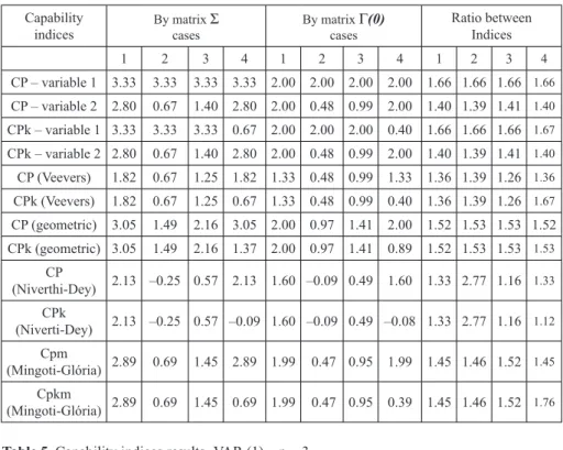
To understand how the autocorrelation affects the process capability values a study was performed under several settings described in Tables 1-3. The models in Table 1 are VAR(1) for p = 2 and p = 3, and VARMA(1,1) for p = 2. Tables 2,3 show the

specification and the process limits for all models of Table 1. For each case and model the capability indices described were calculated based on both matrices Σpxp and Γ(0)

(Tables 4-6). The ratio between the capability results obtained in both situations are presented. For Niverthi and Dey’s indices the global capability process estimate was

defined as the minimum value of the vectors C_pND and C_pkND respectively, as suggested in Mingoti and Glória’s (2008).

The results based on Σpxp matrix ignore the autocorrelation among the observations. On the contrary, the results based on Γ(0) take into account the

autocorrelation. As one can see there is a huge difference between the numerical values of the capability indices calculated under independent and autocorrelated data.

In all cases the capability values based on the matrix Γ(0) are lower (in absolute value) than the values based on Σpxp and in general the differences are larger for Niverthi and Dey’s. When the matrix Γ(0) is used, all the capability indices, except the geometric

mean, were able to recognize the processes which were not capable. The same was

not true when the capability is calculated using the matrix Σpxp (Table 4, cases 3 and 4). The ratio between the capability results calculated with Σpxp and Γ(0) show that the

difference was much larger for VAR(1) with p = 2, than for VAR(1) with p = 3 and VARMA(1,1). Niverthi and Dey’s had the tendency to result in smaller capability values when compared to the other indices.

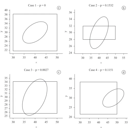
As an illustration in Figure 1a-d, the specification and the process confidence regions (99.73%) are shown for VAR(1) model defined according to Table 2, p = 2. The

probability of non-conforming units with respect to the specification limits are also

presented. Comparing these plots with the capability results of Table 4 we can see that

the capability indices calculated by using matrix Σpxp were completely inappropriate

for case 3 (except Niverthi and Dey’s). The non-capability of case 4 and the possible

non-capability of case 3 are clearly signaled when matrix Γ(0) is used to quantify

the capability. It is important to notice that the numerical values of the multivariate

indices based on Γ(0) discussed in this paper reflect well the condition of the process

in terms of the proportion of non-conforming (p). For case 1, p is approximately zero and all the multivariate capability indices resulted in numerical values larger or equal 1.33; for case 2, p is 0.1532 (153200 ppm) and the multivariate capability indices were lower than 0.5 except for the geometric mean which was equal to 0.97; for case 4 a non-centered process, clearly non-capable in the second variable and with a value of p equals to 0.1151 (115100 ppm) the multivariate capability indices of C_pk type were approximately equal to 0.4 (except the geometric mean that was equal to 0.89).

(9)

V

olume 8, Number

1, 201

1, pp. 133-152

141

Table 1. Parameters matrices for VAR(1), VARMA(1,1) models.

VAR(1)–p = 2

Φ Ψ Σpxp Ppxp Γ(0) ρ(0)

null 1 0 5

0 5 1 .

.

 

 

 

1 0 5

0 5 1

2 906

r

.

C_α .

 

 

 

=

2 78 1 14

1 14 1 96

. .

 

 

 

1 0 487

0 487 1

3 014

r

.

C_α .

 

 

 

=

VAR (1)–p = 3

0 5 0 0

0 0 7 0

0 0 0 3

. . .           null

1 0 5 0 7

0 5 1 0 3

0 7 0 3 1

. . . . . .          

1 0 5 0 7

0 5 1 0 3 0 7 0 3 1

3 041

r

. .

C_α .

          =

1 33 0 77 0 82 0 77 1 96 0 38

0 82 0 38 1 09

. . . . . . . . .          

1 0 476 0 680

0 476 1 0 259 0 680 0 259 1

3 146

r

. .

C_α .

          =

VARMA (1,1)–p = 2

Φ H Σ_pxp P_pxp Γ(0) ρ(0)

0 9 0

0 0 1 .

.

 

 

 

0 7 0

0 0 1 .

.

 

 

 

1 0 5

0 5 1 .

.

 

 

 

1 0 5

0 5 1

2 944

r

.

C_α .

 

 

 

=

1 21 0 5

0 5 1

. .

.

 

 

 

1 0 454

0 454 1

2 972

r

.

C_α .

 

 

 

=

0 8 0

0 0 7 .

.

 

 

(10)

variable are equal to the process limits, the value of p is 0.0027 (2700 ppm) and the multivariate capability indices were lower but close to 1, except Niverthi and Dey’s which resulted the value 0.49.

From the results in Tables 4-6 it is clear that Niverthi and Dey’s penalizes the processes more than the other indices even when the probability of non-conforming process units is small (see case 3 whose proportion of non-conforming process units

according to the specification limits is 0.0027). Due to this tendency it is possible that a

capable process will be considered non-capable by Niverthi and Dey´s indices (Mingoti and Glória, 2008). On the other hand, Mingoti and Glória’s and Veevers’ were more stable and produced more suitable information about the true capability (capability values close to 1 for case 3).

Example of Application

When data is collected from a multivariate normal process with the purpose

of estimating its capability the first step is to verify if the autocorrelation is present

in the data and then to identify the appropriate time series model that is generating

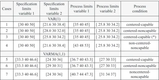
Table 2. Specification and process limits – p = 2.

Cases

Specification

limits variable 1

Specification

limits variable 2

Process limits variable 1

Process limits variable 2

Process condition VAR(1)

1 [30 40 50] [21.6 30 38.4] [35 40 45] [ 25.8 30 34.2] centered-capable 2 [30 40 50] [28.0 30 32.0] [35 40 45] [ 25.8 30 34.2] centered-noncapable 3 [30 40 50] [25.8 30 34.2] [35 40 45] [ 25.8 30 34.2] centered-capable (*) 4 [30 40 50] [21.6 30 38.4] [43 48 53] [ 25.8 30 34.2]

non-centered-noncapable VARMA(1,1)

5 [33.3 40 46.6] [24 30 36] [36.7 40 43.3] [27 30 33] centered-capable 6 [33.3 40 46.6] [29 30 31] [36.7 40 43.3] [27 30 33] centered-noncapable 7 [33.3 40 46.6] [24 30 36] [40.7 44 47.3] [31 34 37]

noncentered-noncapable

*This process is barely capable in the second variable.

Table 3. Specification and process limits – VAR(1) – p = 3.

Parameters Case 8 Case 9 Case 10

Specification limits – variable 1 [33.0 40 47.0] [33.0 40 47.0] [33.0 40 47.0]

Specification limits – variable 2 [21.6 30 38.4] [21.6 30 38.4] [21.6 30 38.4]

Specification limits – variable 3 [13.6 20 26.4] [13.6 20 26.4] [13.6 20 26.4] Process limits – variable 1 [36.5 40 43.5] [42.5 46 49.5] [42.5 46 49.5] Process limits – variable 2 [25.7 30 34.3] [26.8 31 35.2] [30.8 35 39.2] Process limits – variable 3 [16.8 20 23.2] [16.8 20 23.2] [20.8 24 27.2]

Process condition centered-capable

(11)

Volume 8, Number 1, 2011, pp. 133-152

143

Figure 1. Elipses (99.73%) and the specification region – Var(1), bivariate, p = probability of

non-conforming units according to the specification limits.

a b

c d

the observations. After the parameters of the model are estimated the values of any

capability index presented in this paper can be calculated since the matrices Φ, Σpxp and Γ(0) are estimated by maximum likelihood or other methods (Lutkepohl, 2005). As an

(12)

Table 5. Capability indices results- VAR (1) – p = 3.

Capability index By matrix Σ cases

By matrix Γ(0) cases

Ratio between indices

8 9 10 8 9 10 8 9 10

CP – variable 1 2.33 2.33 2.33 2.02 2.02 2.02 1.15 1.15 1.15 CP – variable 2 2.80 2.80 2.80 2.00 2.00 2.00 1.40 1.41 1.41 CP – variable 3 2.13 2.13 2.13 2.03 2.03 2.03 1.05 1.05 1.05 CPk – variable 1 2.33 0.33 0.33 2.02 0.29 0.29 1.15 1.14 1.14 CPk – variable 2 2.80 2.47 1.13 2.00 1.76 0.81 1.40 1.40 1.40 CPk – variable 3 2.13 2.13 0.8 2.03 2.04 0.76 1.05 1.04 1.05 CP (Veevers) 1.25 1.24 1.24 1.15 1.15 1.15 1.09 1.08 1.08 CPk (Veevers) 1.25 0.33 0.27 1.15 0.29 0.18 1.09 1.14 1.50 CP (geometric) 2.41 2.41 2.41 2.02 2.02 2.02 1.19 1.19 1.19 CPk (geometric) 2.41 1.21 0.67 2.02 1.01 0.56 1.19 1.20 1.20 CP (Niverthi-Dey) 1.33 1.33 1.33 1.17 1.18 1.17 1.14 1.13 1.14 CPk (Niverti-Dey) 1.33 –1.41 –0.30 1.17 –1.14 –0.23 1.14 1.24 1.30

Cpm

(Mingoti-Glória) 2.10 2.03 2.03 1.91 1.97 1.97 1.10 1.03 1.03 Cpkm

(Mingoti-Glória) 2.10 0.32 0.32 1.91 0.28 0.28 1.10 1.14 1.14

Table 4. Capability indices results – VAR(1) – p = 2.

Capability indices

By matrix Σ cases

By matrix Γ(0)

cases

Ratio between Indices 1 2 3 4 1 2 3 4 1 2 3 4 CP – variable 1 3.33 3.33 3.33 3.33 2.00 2.00 2.00 2.00 1.66 1.66 1.66 1.66

CP – variable 2 2.80 0.67 1.40 2.80 2.00 0.48 0.99 2.00 1.40 1.39 1.41 1.40

CPk – variable 1 3.33 3.33 3.33 0.67 2.00 2.00 2.00 0.40 1.66 1.66 1.66 1.67

CPk – variable 2 2.80 0.67 1.40 2.80 2.00 0.48 0.99 2.00 1.40 1.39 1.41 1.40

CP (Veevers) 1.82 0.67 1.25 1.82 1.33 0.48 0.99 1.33 1.36 1.39 1.26 1.36

CPk (Veevers) 1.82 0.67 1.25 0.67 1.33 0.48 0.99 0.40 1.36 1.39 1.26 1.67

CP (geometric) 3.05 1.49 2.16 3.05 2.00 0.97 1.41 2.00 1.52 1.53 1.53 1.52 CPk (geometric) 3.05 1.49 2.16 1.37 2.00 0.97 1.41 0.89 1.52 1.53 1.53 1.53

CP

(Niverthi-Dey) 2.13 –0.25 0.57 2.13 1.60 –0.09 0.49 1.60 1.33 2.77 1.16 1.33 CPk

(Niverti-Dey) 2.13 –0.25 0.57 –0.09 1.60 –0.09 0.49 –0.08 1.33 2.77 1.16 1.12 Cpm

(Mingoti-Glória) 2.89 0.69 1.45 2.89 1.99 0.47 0.95 1.99 1.45 1.46 1.52 1.45 Cpkm

(13)

Volume 8, Number 1, 2011, pp. 133-152

145

 

₀

0 6501 0 0089 0 0325 0 0135

0 0017 0 7467 0 0135 0 0110

0 0568 0 0264 1 0 669

0

0 0264 0 0247 0 669 1

. – . . – .

;

. . – . .

. – . – .

; p( )

– . . – .

   

Φ =_ _ Σ =_ _

   

   

Γ =_ _ =_ _

    

(20)



₍

₎

 

0

0 6525 0 0000

21 1618 6 1597 0 0000 0 7428

0 0322 0 0134 0 0561 0 0260 1 0 680

0 0134 0 0109 0 0260 0 0244 0 680 1

. .

; . ; . ;

. .

. – . . – . – .

; (0)

– . . – . .

r

– .

 

Φ =_ _ m =

 

     

Σ =_ _Γ =_ _ =_ _

     



(21)

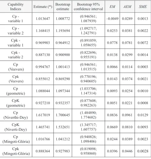
where r^(0) is the estimated correlation matrix based on Γ0and m^0 is the process vector mean estimate. For a confidence level of 99.73% (i.e. α = 0.0027) the constant m is 3 and C_r_α is 3.014. The capability estimates are shown in Table 7. As one can see the non-capability condition of the process is signaled by the C_pk univariate indices as well as by their geometric means. Among the other multivariate capability indices Veevers’ and Mingoti and Glória’s were more sensitive to the non-capability condition of the process. On the contrary, Niverthi and Dey’s indices were not able to signal the non-capability given numerical values larger than 1.

The bootstrap methodology (Efron and Tibashirani, 1993) was used

to generate confidence intervals for the true process capability indices for each

Table 6. Capability indices results - VARMA (1,1) – p = 2.

Capability index By matrix Σ cases By matrix Γ(0) cases Ratio between indices

5 6 7 5 6 7 5 6 7

(14)

methodology. A total of m = 1000 bootstrap samples of sizes n = 360 were selected with replacement. For each bootstrap sample the estimates of all multivariate capability

indices discussed in this paper were calculated at α = 0.0027 and compared to the corresponding bootstrap values of Table 7. The mean error (ME), the absolute mean error (AME) and the squared mean error (SME) were calculated (see Table 7 for the results). As we can see the ME, AME and the SME values were larger for Niverthi and Dey estimates than for Mingoti and Glória, the geometric means and Veevers indices. All indices are practically unbiased (mean errors close to zero) and their distributions

(15)

Volume 8, Number 1, 2011, pp. 133-152

147

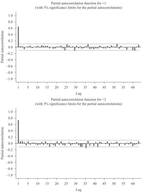
Figure 3. Partial autocorrelation of the blast charcoal furnace of pig iron production series.

resemble the univarite normal except Veevers C_p (Figure 4). For all multivariate indices,

except Niverthi and Dey, the 95% bootstrap confidence limits for the true capability

show that the process is non-capable since the upper limit is lower or very close to

1. The lower limits of the confidence interval built using Niverthi and Dey’s indices

were very far from 1 giving no sign at all of the non-capability of the process. The

confidence interval using Mingoti and Glória’s, Cm

pk , resulted in smaller range (0.139)

(16)

Final Remarks

This paper shows the importance of taking into account the autocorrelation of the process in the calculation of capability multivariate indices. As we have shown, in the presence of autocorrelation a non-capable process may be considered capable if the capability index is not properly corrected. In a real situation the user needs to collect enough data to correctly identify the multivariate time series model which had generated the observations of the process. For a VAR(1) model the routine mAr.est from the software R for windows may be used to estimate the matrices Φ_pxp, Σ_pxp, Γ(0) and

ρ(0). The estimation procedure is based upon a minimum squares stepwise (Neumaier and Schneider, 2001). The user can also make its own program to obtain a maximum likelihood solution (Lutkepohl, 2005). By doing so any capability multivariate index

(17)

Volume 8, Number 1, 2011, pp. 133-152

149

discussed in this paper can be calculated. Confidence intervals for the true capability

index can also be built by using the bootstrap methodology as an alternative.

The results of this paper had shown that Veever’s and Mingoti and Glória’s multivariate capability indices performed better than Niverthi and Dey’s and were less subject to wrong conclusions about the capability or non-capability of the process. Since they are even easier to calculate they should be preferred.

Finally, in this paper for VAR(1) and p = 2 it was presented the correspondence between the capability index value and the probability (p) of non-conforming units

generated by the process according to the specification limits. As a future work it would

be interesting to establish some reference values for the multivariate indices to be used to classify the process capability in bands similar as done for univariate processes.

Table 7. Estimate capability and bootstrap results for the blast charcoal furnace example.

Capability

Indices Estimate (*)

Bootstrap estimate

Bootstrap 95%

confidence interval EM AEM SME

Cp -

variable 1 1.013647 1.008772

(0.946561;

1.087939) –0.0049 0.0289 0.0013

Cp -

variable 2 1.168415 1.193694

(1.092717;

1.242791) 0.0253 0.0381 0.0022

Cpk -

variable 1 0.969903 0.964912

(0.891059;

1.058655) 0.0778 0.0781 0.0072 Cpk -

variable 2 0.887130 0.900900

(0.822696;

0.955191) 0.0138 0.0299 0.0014

Cp

(Veevers) 0.994767 1.001413

(0.946561;

1.013515) 0.0066 0.0114 0.0003 Cpk

(Veevers) 0.855012 0.869290

(0.770196;

0.940605) 0.0143 0.0374 0.0021

Cp

(geometric) 1.088044 1.097344

(1.033706;

1.147314) 0.0093 0.0254 0.0010

CpK

(geometric) 0.927210 0.932357

(0.877608;

0.982263) 0.0051 0.0221 0.0008

Cp

(Niverthi-Dey) 1.617019 1.700645

(1.484890;

1.774682) 0.0836 0.0961 0.0129

CpK

(Niverti-Dey) 1.465741 1.532651

(1.345717;

1.607757) 0.0669 0.0810 0.0093

Cp

(Mingoti-Glória) 1.016766 1.041212

(0.940826;

1.098406) 0.0244 0.0389 0.0023

Cpk

(Mingoti-Glória) 0.888364 0.927983

(0.819098;

0.958860) 0.0396 0.0446 0.0028

(18)

Acknowledgments

The authors were partially supported by the Brazilian institutions:

CAPES-High Level Staff Improvement Coordination and CNPq- National Council for Scientific

and Technological Development.

References

Alwan, L.C. and Roberts, H.V. (1995) The Problem of Misplaced Control Limits. Applied Statistics, Vol. 44, No. 3, pp. 269-278. http://dx.doi.org/10.2307/2986036

Bernardo, J.M. and Irony, T.X. (1996) A General Multivariate Bayesian Process Capability Index. Statistician, Vol. 45, pp. 487-502. http://dx.doi.org/10.2307/2988547

Chan, L.K.; Chen, S.W. and Spiring, F.A. (1991) A Multivariate Measure of Process Capability. International. Journal of Modeling and Simulation, Vol. 11, No. 1, pp. 1-6.

Chen, H. (1994) A Multivariate Process Capability Index Over a Rectangular Solid Tolerance Zone. Statistica Sinica, Vol. 4, No. 2, pp.749-758.

Cheng, S.W. and Spiring, F.A. (1989) Assessing Process Capability: A Bayesian Approach. IIE Transactions, Vol. 21, pp. 97-98. http://dx.doi.org/10.1080/07408178908966212

Efron, B. and Tibshirani, R.J. (1993) An Introduction to the Bootstrap. New York: Chapman and Hall.

Hayter, A.J. and Tsui, K-L. (1994) Identification and Quantification in Multivariate Quality Control Problems. Journal of Quality Technology, Vol. 26, No. 3, pp.197-208.

Hotelling, H. (1947), Multivariate quality control, in: Eisenhart, M.; Hastay, W. and Wallis, A. (Eds.), Techniques of Statistical Analysis. New York: MacGraw-Hill, pp. 111-184.

Jarret, J. and Pan, X. (2007) The Quality Control Chart for Monitoring Multivariate Autocorrelated Processes. Computational Statistics and Data Analysis, Vol. 51, No. 8, pp. 3862-3870. http://dx.doi.org/10.1016/j.csda.2006.01.020

Kalgonda, A.A. and Kulkarni, S.R. (2004) Multivariate Quality Control Chart for Autocorrelated Processes. Journal of Applied Statistics, Vol. 31, No. 3, pp.317-327. http://dx.doi. org/10.1080/0266476042000184000

Koltz, S. and Johnson, N.L. (2002) Process Capability Indices-A Review. 1992-2000. Journal of Quality Technology, Vol. 34, No. 1, pp. 2-39.

Koltz, S. and Johnson, N.L. (1993), Process Capability Indices. London: Chapman and Hall.

Kramer, H.G. and Schmid, W. (1997) EWMA Charts for Multivariate Time Series. Sequential Analysis, Vol. 16, No. 2, pp. 131-154. http://dx.doi.org/10.1080/07474949708836378

Lutkepohl, H. (2005), Introduction to Multiple Time Series Analysis. Berlin: Springer Verlag.

Mason, R.L. and Young, J.C. (2002) Multivariate Statistical Process Control with Industrial Applications. Alexandria: American Statistics Society. http://dx.doi. org/10.1137/1.9780898718461

Mingoti, S.A. and Glória, F.A.A. (2008) Comparing Mingoti and Glória´s and Niverthi and Dey´s Multivariate Capability Indices. Produção, Vol. 18, No. 3, pp. 598-608. http:// dx.doi.org/10.1590/S0103-65132008000300014

(19)

Volume 8, Number 1, 2011, pp. 133-152

151

Niverthi, M. and Dey, D.K. (2000) Multivariate Process Capability: A Bayesian Perspective. Communications in Statistics-Simulation and Computation, Vol. 29, No. 2, pp.667-687. http://dx.doi.org/10.1080/03610910008813634

Pearn, W.L.; Wang, F.K. and Yen, C.H. (2007) Multivariate Capability Indices: Distributional and Inferential Properties. Journal of Applied Statistics, Vol. 34, No. 8, pp. 941-962. http://dx.doi.org/10.1080/02664760701590475

Shahriari, H.; Hubele, N.F. and Lawrence, F.P. (1995) A Multivariate Process Capability Vector, in: Industrial Engineering Research Conference, Institute of Industrial Engineers, pp. 304-309.

Taam, W.; Subbaiha, P. and Liddy, J.W. (1993) A Note on Multivariate Capability Indices. Journal of Applied Statistics, Vol. 20, No. 3, pp.339-351. http://dx.doi. org/10.1080/02664769300000035

Veevers, A. (1998) Viability and Capability Indices for Multiresponse Processes. Journal of Applied Statistics, Vol. 25, No. 4, pp.545-558. http://dx.doi.org/10.1080/02664769823016

Wang, F.K.; Hubele, N.F.; Lawrence, F.P.; Miskulin, J.O. and Shariari, H. (2000) Comparison of three Multivariate Process Capability Indices. Journal of Quality Technology, Vol. 32, No. 3, pp. 263-275.

Zhang, N.Z. (1998) Estimating Process Capability Indices for Autocorrelated Data. Journal of Applied Statistics, Vol. 25, No. 4, pp.559-574. http://dx.doi.org/10.1080/02664769823025

Biography

Sueli Aparecida Mingoti is an Associate Professor at the Statistics Departament of Federal University of Minas Gerais (UFMG),Brazil. She received her Ph.D degree in Statistics from the Iowa State University located at Ames, United States of America, in 1989. Her research interests includes applied probability and inference, multivariate and industrial statistics.

Contact: sueliam@est.ufmg.br

Fernando Luiz Pereira de Oliveira received his D.Sc. from the Department of Statistics at Federal University of Minas Gerais, in 2011. Since then he has been serving on the Department of Mathematics at Federal University of Ouro Preto (UFOP), Minas Gerais, Brazil. His major interests are process capability, statistical quality control and clusters detection.

Contact: fernandoluiz@iceb.ufop.br

Article Info:

Received: May, 2010

(20)