EFFECTIVENESS PREDICTION OF MEMORY BASED CLASSIFIERS FOR THE CLASSIFICATION OF MULTIVARIATE DATA SET

(1)

Sundarapandian et al. (Eds): CoNeCo,WiMo, NLP, CRYPSIS, ICAIT, ICDIP, ITCSE, CS & IT 07, pp. 413–424, 2012. © CS & IT-CSCP 2012 DOI : 10.5121/csit.2012.2440

C. Lakshmi Devasena

1

Department of Computer Science and Engineering, Sphoorthy Engineering College, Hyderabad, India

devaradhe2007@gmail.com

A

BSTRACT

Classification is a step by step practice for allocating a given piece of input into any of the given category. Classification is an essential Machine Learning technique. There are many classification problem occurs in different application areas and need to be solved. Different types are classification algorithms like memory-based, tree-based, rule-based, etc are widely used. This work studies the performance of different memory based classifiers for classification of Multivariate data set from UCI machine learning repository using the open source machine learning tool. A comparison of different memory based classifiers used and a practical guideline for selecting the most suited algorithm for a classification is presented. Apart from that some empirical criteria for describing and evaluating the best classifiers are discussed.

K

EYWORDS

Classification, IB1 Classifier, IBk Classifier, K Star Classifier, LWL Classifier

1. I

NTRODUCTION

In machine learning, classification refers to an algorithmic process for designating a given input data into one among the different categories given. An example would be a given program can be assigned into "private" or "public" classes. An algorithm that implements classification is known as a classifier. The input data can be termed as an instance and the categories are known as classes. The characteristics of the instance can be described by a vector of features. These features can be nominal, ordinal, integer-valued or real-valued. Many data mining algorithms work only in terms of nominal data and require that real or integer-valued data be converted into groups.

(2)

2. L

ITERATURE

R

EVIEW

In [1], the comparison of the performance analysis of Fuzzy C mean (FCM) clustering algorithm with Hard C Mean (HCM) algorithm on Iris flower data set is done and concluded Fuzzy clustering are proper for handling the issues related to understanding pattern types, incomplete/noisy data, mixed information and human interaction, and can afford fairly accurate solutions faster. In [6], the issues of determining an appropriate number of clusters and of visualizing the strength of the clusters are addressed using the Iris Data Set.

3. D

ATA SET

IRIS flower data set classification problem is one of the novel multivariate dataset created by Sir Ronald Aylmer Fisher [3] in 1936. IRIS dataset consists of 150 instances from three different types of Iris plants namely Iris setosa, Iris virginica and Iris versicolor, each of which consist of 50 instances. Length and width of sepal and petals is measured from each sample of three selected species of Iris flower. These four features were measured and used to classify the type of plant are the Sepal Length, Petal Length, Sepal Width and Petal Width [4]. Based on the combination of the four features, the classification of the plant is made. Other multivariate datasets selected for comparison are Car Evaluation Dataset and 1984 United States Congressional Voting Records Dataset from UCI Machine Learning Repository [8]. Car Evaluation dataset has six attributes and consists of 1728 instances of four different classes. Congressional Voting Records Dataset has 16 attributes and consists of 435 instances of two classes namely Democrat and Republican.

4. C

LASSIFIERS

U

SED

Different memory based Classifiers are evaluated to find the effectiveness of those classifiers in the classification of Iris Data set. The Classifiers evaluated here are.

4.1. IB1 Classifier

IB1 is nearest neighbour classifier. It uses normalized Euclidean distance to find the training instance closest to the given test instance, and predicts the same class as this training instance. If several instances have the smallest distance to the test instance, the first one obtained is used. Nearest neighbour method is one of the effortless and uncomplicated learning/classification algorithms, and has been effectively applied to a broad range of problems [5].

To classify an unclassified vector X, this algorithm ranks the neighbours of X amongst a given set of N data (Xi, ci), i = 1, 2, ...,N, and employs the class labels cj (j = 1, 2, ...,K) of the K most similar neighbours to predict the class of the new vector X. In specific, the classes of the K neighbours are weighted using the similarity between X and its each of the neighbours, where the Euclidean distance metric is used to measure the similarity. Then, X is assigned the class label with the greatest number of votes among the K nearest class labels. The nearest neighbour classifier works based on the intuition that the classification of an instance is likely to be most similar to the classification of other instances that are nearby to it within the vector space. Compared to other classification methods such as Naive Bayes’, nearest neighbour classifier does not rely on prior probabilities, and it is computationally efficient if the data set concerned is not very large.

4.2. IBk Classifier

(3)

For example, for the ‘iris’ data, IBK would consider the 4 dimensional space for the four input variables. A new instance would be classified as belonging to the class of its closest neighbour using Euclidean distance measurement. If 5 is used as the value of ‘k’, then 5 closest neighbours are considered. The class of the new instance is considered to be the class of the majority of the instances. If 5 is used as the value of k and 3 of the closest neighbours are of type ‘Iris-setosa’, then the class of the test instance would be assigned as ‘Iris-setosa’. The time taken to classify a test instance with nearest-neighbour classifier increases linearly with the number of training instances kept in the classifier. It has a large storage requirement. Its performance degrades quickly with increasing noise levels. It also performs badly when different attributes affect the outcome to different extents. One parameter that can affect the performance of the IBK algorithm is the number of nearest neighbours to be used. By default it uses just one nearest neighbour.

4.3. K Star Classifier

KStar is a memory-based classifier that is the class of a test instance is based upon the class of those training instances similar to it, as determined by some similarity function. The use of entropy as a distance measure has several benefits. Amongst other things it provides a consistent approach to handling of symbolic attributes, real valued attributes and missing values. K* is an instance-based learner which uses such a measure [6].

Specification of K*

Let I be a (possibly infinite) set of instances and T a finite set of transformations on I. Each t ∈T maps instances to instances: t: I I. T contains a distinguished member (the stop symbol) which for completeness maps instances to themselves ( (a) = a). Let P be the set of all prefix codes from T* which are terminated by . Members of T* (and so of P) uniquely define a transformation on I: t(a) = tn (tn-1 (... t1(a) ...)) where t = t1,...tn

A probability function p is defined on T*. It satisfies the following properties:

(1)

As a consequence it satisfies the following:

(2)

The probability function P* is defined as the probability of all paths from instance ‘a’ to instance ‘b’:

(3)

(4)

The K* function is then defined as:

(5)

K* is not strictly a distance function. For example, K*(a|a) is in general non-zero and the function (as emphasized by the | notation) is not symmetric. Although possibly counter-intuitive the lack of these properties does not interfere with the development of the K* algorithm below. The following properties are provable:

(6).

4.4. LWL Classifier

LWL is a learning model that belongs to the category of memory based classifiers. Machine Learning Tools work by default with LWL model and Decision Stump in combination as classifier. Decision Stump usually is used in conjunction with a boosting algorithm.

Boosting is one of the most important recent developments in classification methodology. Boosting works by sequentially applying a classification algorithm to reweighted versions of the training data, and then taking a weighted majority vote of the sequence of classifiers thus produced. For many classification algorithms, this simple strategy results in dramatic improvements in performance. This seemingly mysterious phenomenon can be understood in terms of well known statistical principles, namely additive modelling and maximum likelihood. For the two-class problem, boosting can be viewed as an approximation to additive modelling on the logistic scale using maximum Bernoulli likelihood as a criterion. We are trying to find the best estimate for the outputs, using a local model that is a hiper-plane. Distance weighting the data training points corresponds to requiring the local model to fit nearby points well, with less concern for distant points:

(7)

This process has a physical interpretation. The strength of the springs are equal in the unweighted case, and the position of the hiper-plane minimizes the sum of the stored energy in the springs (Equation 8). We will ignore a factor of 1/2 in all our energy calculations to simplify notation. The stored energy in the springs in this case is C of Equation 7, which is minimized by the physical process.

(8)

(5)

In what follows we will assume that the constant 1 has been appended to all the input vectors xi to

include a constant term in the regression. The data training points can be collected in a matrix equation:

Xβ = y (10)

where X is a matrix whose ith row is xiT and y is a vector whose i th

element is yi . Thus, the

dimensionality of X is ‘n x d’ where n is the number of data training points and d is the dimensionality of x. Estimating the parameters using an unweighted regression minimizes the criterion given in equation 1 [7]. By solving the normal equations

(XTX) β = XT y (11)

For β: β = (XTX) - iXTy (12)

Inverting the matrix XTX is not the numerically best way to solve the normal equations from the point of view of efficiency or accuracy, and usually other matrix techniques are used to solve Equation 11.

5. C

RITERIA

U

SED FOR

C

OMPARISON

E

VALUATION

The comparison of the results is made on the basis of the following criteria.

5.1. Accuracy Classification

All classification result could have an error rate and it may fail to classify correctly. So accuracy can be calculated as follows.

Accuracy = (Instances Correctly Classified / Total Number of Instances)*100 % (13)

5.2. Mean Absolute Error

MAE is the average of difference between predicted and actual value in all test cases. The formula for calculating MAE is given in equation shown below:

MAE = (|a1 – c1| + |a2 – c2| + … +|an – cn|) / n (14)

Here ‘a’ is the actual output and ‘c’ is the expected output.

5.3. Root Mean Squared Error

RMSE is used to measure differences between values predicted by a model and the values actually observed. It is calculated by taking the square root of the mean square error as shown in equation given below:

(15)

(6)

5.4. Confusion Matrix

A confusion matrix contains information about actual and predicted classifications done by a classification system.

The classification accuracy, mean absolute error, root mean squared error and confusion matrices are calculated for each machine learning algorithm using the machine learning tool.

6. R

ESULTS AND

D

ISCUSSION

This work is performed using Machine learning tool to evaluate the effectiveness of all the memory- based classifiers for various multivariate datasets.

Data Set 1: Iris Data set

The performance of the these algorithms measured in Classification Accuracy, RMSE and MAE values as shown in Table 1. Comparison among these classifiers based on the correctly classified instances is shown in Fig. 1. Comparison among these classifiers based on MAE and RMSE values are shown in Fig. 2. The confusion matrix arrived for these classifiers are shown from Table 2 to Table 5. The overall ranking is done based on the classification accuracy, MAE and RMSE values and it is given in Table 1. Based on the results arrived, IB1Classifier which has 100% accuracy and 0 MAE and RMSE got the first position in ranking followed by IBk, K Star and LWL as shown in Table 1.

100 110 120 130 140 150

IB1 Ibk K S tar LWL

Te chni que s Use d

C ompari son base d on C orre ctly C l assifie d In stance s

C orre ctly C l assifie d Incorre ctly C lassifie d

(7)

0 0.02 0.04 0.06 0.08 0.1 0.12 0.14 0.16 0.18

IB1 IBk K Star LWL

Techniques Used Comparison based on MAE and RMSE

Mean Absolute Error Root Mean Squared Error

Figure 2. Comparison based on MAE and RMSE values – Iris Dataset

Table 1. Overall Results of Memory Based Classifiers – IRIS Dataset

Classifier Used

Instances Correctly Classified (Out of 150)

Classification Accuracy (%)

MAE RMSE Rank

IB1 150 100 0 0 1

IBk 150 100 0.0085 0.0091 2

K Star 150 100 0.0062 0.0206 3

LWL 147 98 0.0765 0.1636 4

Table 2. Confusion Matrix for IB1 Classifier – IRIS Dataset

A B C

A = Iris-Setosa 50 0 0 B = Iris-Versicolor 0 50 0 C = Iris-Virginica 0 0 50

Table 3. Confusion Matrix for IBk Classifier – IRIS Dataset

A B C

Table 4. Confusion Matrix for K*Classifier – IRIS Dataset

A B C

(8)

Table 5. Confusion Matrix for LWL Classifiers – IRIS Dataset

A B C

Data Set 2: Car Evaluation Data set

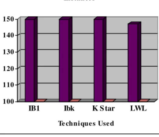
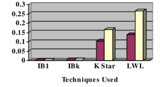
The performance of the these algorithms measured for Car Evaluation Data set in terms of Classification Accuracy, RMSE and MAE values as shown in Table 6. Comparison among the classifiers based on the correctly classified instances is shown in Fig. 3. Comparison among these classifiers based on MAE and RMSE values are shown in Fig. 4. The confusion matrix arrived for these classifiers are shown from Table 7 to Table 10. The overall ranking is done based on the classification accuracy, MAE and RMSE values and it is given in Table 6. Based on the results arrived, IB1 Classifier has 100% accuracy and 0 MAE and RMSE got the first position in ranking followed by IBk, K Star and LWL as shown in Table 6.

0 200 400 600 800 1000 1200 1400 1600 1800

IB1 Ibk K Star LWL

Techniques Used

Comparison based on Correctly Classified Insances

Correctly Classified Incorrecly Classified

Figure 3. Comparison based on Number of Instances Correctly Classified – CAR Dataset

0 0.05 0.1 0.15 0.2 0.25 0.3

IB1 IBk K Star LWL

Te chn ique s Use d C omparison base d on MAE and RMSE

Me an Absol ute Error Root Me an Square d Error

(9)

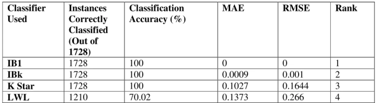
Table 6. Overall Results of Memory Based Classifiers – CAR Dataset

Instances Correctly Classified (Out of 1728)

IB1 1728 100 0 0 1

IBk 1728 100 0.0009 0.001 2

K Star 1728 100 0.1027 0.1644 3

LWL 1210 70.02 0.1373 0.266 4

Table 7. Confusion Matrix for IB1Classifier – CAR Dataset

A B C D

A = Unaccident 1210 0 0 0 B = Accident 0 384 0 0 C = Good 0 0 69 0 D = Verygood 0 0 0 65

Table 8. Confusion Matrix for IBk Classifier – CAR Dataset

A B C D

Table 9. Confusion Matrix for K Star Classifier – CAR Dataset

A B C D

Table 10. Confusion Matrix for LWL Classifier – CAR Dataset

A B C D

Data Set 3: Congressional Voting Records Data set

(10)

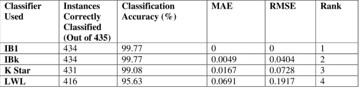
among these classifiers based on MAE and RMSE values are shown in Fig. 6. The confusion matrix arrived for these classifiers are shown from Table 12 to Table 15. The overall ranking is done based on the classification accuracy, MAE and RMSE values and it is given in Table 11. Based on the results arrived, IB1 Classifier has 99.77% accuracy and 0 MAE and RMSE got the first position in ranking followed by IBk, K Star and LWL as shown in Table 11.

0 50 100 150 200 250 300 350 400 450

IB1 Ibk K Star LWL

Techniques Used

Comparison based on Correctly Classified Instances

Correctly Classified Incorrectly Classified

Figure 5. Comparison based on Number of Instances Correctly Classified – VOTE Dataset

0 0.05 0.1 0.15 0.2

IB1 IBk K Star LWL

Techniques Used Comparison based on MAE and RMSE

Mean Absolute Error Root Mean Squared Error

(11)

Table 11. Overall Results of Memory Based Classifiers – VOTE Dataset

Instances Correctly Classified (Out of 435)

IB1 434 99.77 0 0 1

IBk 434 99.77 0.0049 0.0404 2

K Star 431 99.08 0.0167 0.0728 3

LWL 416 95.63 0.0691 0.1917 4

Table 12. Confusion Matrix for IB1Classifier – VOTE Dataset

A B

A = Democrat 267 0 B = Republican 1 167

Table 13. Confusion Matrix for IBk Classifier – VOTE Dataset

A B

Table 14. Confusion Matrix for K Star Classifier – VOTE Dataset

A B

Table 15. Confusion Matrix for LWL Classifier – VOTE Dataset

A B

7. C

ONCLUSIONS

(12)

A

CKNOWLEDGEMENTS

The author thanks the Management and Faculties of CSE Department of Sphoorthy Engineering College for the cooperation extended.

R

EFERENCES

[1] Pawan Kumar and Deepika Sirohi, “Comparative Analysis of FCM and HCM Algorithm on Iris Data Set,” International Journal of Computer Applications, Vol. 5, No.2, pp 33 – 37, August 2010.

[2] David Benson-Putnins, Margaret monfardin, Meagan E. Magnoni, and Daniel Martin, “Spectral Clustering and Visualization: A Novel Clustering of Fisher's Iris Data Set”.

[3] Fisher, R.A, “The use of multiple measurements in taxonomic problems” Annual Eugenics, 7, pp.179 – 188, 1936.

[4] Patrick S. Hoey, “Statistical Analysis of the Iris Flower Dataset”.

[5] M. Kuramochi, G. Karypis. “Gene classification using expression profiles: a feasibility study”, International Journal on Artificial Intelligence Tools, 14(4):641-660, 2005.

[6] John G. Cleary, “K*: An Instance-based Learner Using an Entropic Distance Measure.

[7] Christopher G. Atkeson, Andrew W. Moore and Stefan Schaal, “Locally Weighted Learning” October 1996.

[8] UCI Machine Learning Data Repository – http://archive.ics.uci.edu/ml/datasets.

Authors