Variance Premium and Implied Volatility in
a Low-Liquidity Option Market
*
Eduardo Sanchez Astorino
†
Fernando Chague
‡
Bruno Giovannetti
§
Marcos Eugênio da Silva
¶
Contents: 1. Introduction; 2. Implied volatility index for the Brazilian stock market; 3. Empirical analysis using the IVol-BR; 4. Conclusion; Appendix.
Keywords: Volatility Index, Predictability, Risk Aversion, Equity Variance Premium JEL Code: G12, G13, G17.
We propose an implied volatility index for Brazil that we name “IVol-BR”. The index is based on daily market prices of options over Ibovespa—an option mar-ket with relatively low liquidity and few option strikes. Our methodology com-bines standard international methodology used in high-liquidity markets with adjustments that take into account the low liquidity in Brazilian option mar-kets. We do a number of empirical tests to validate the IVol-BR. First, we show that the IVol-BR has significant predictive power over future volatility of equity returns not contained in traditional volatility forecasting variables. Second, we decompose the squared IVol-BR into (i) the expected variance of stock returns and (ii) the equity variance premium. This decomposition is of interest since the equity variance premium directly relates to the representative investor risk aversion. Finally, assumingBollerslev, Tauchen, & Zhou(2009) functional form, we produce a time-varying risk aversion measure for the Brazilian investor. We empirically show that risk aversion is positively related to expected returns, as theory suggests.
Nós propomos um índice de volatilidade implícita para o mercado acionário do Bra-sil que chamamos de “IVol-BR”. O índice é baseado nos preços diários das opções
*We thank Fausto Araújo, Alan De Genaro Dario, Rodrigo De-Losso, Eduardo Luzio and José Carlos de Souza Santos for great
discussion and inputs about this paper. We also thank the Editor (José Fajardo) and two anonymous referees for their comments. All errors left are our own.
†Faculdade de Economia, Administração e Contabilidade da Universidade de São Paulo (FEA-USP). Av. Prof. Luciano Gualberto, 908,
Cidade Universitária, São Paulo, SP, Brasil. CEP 05508-010. Email:[email protected] ‡FEA-USP. Email:[email protected]
§FEA-USP. Email:[email protected]
sobre o Ibovespa—um mercado de opções com liquidez relativamente baixa e pou-cos preços de exercício. Nossa metodologia combina a metodologia internacional pa-drão usada em mercados de alta liquidez com ajustes que levam em conta a baixa liquidez do mercado brasileiro. Conduzimos uma variedade de testes empíricos a fim de validar o IVol-BR. Em primeiro lugar, demonstramos que o IVol-BR possui um poder de previsão significativo sobre a volatilidade futura do retorno do Ibovespa que não é encontrado em variáveis de previsão de volatilidade tradicionais. Em se-gundo lugar, decompomos o quadrado do IVol-BR em (i) a variância esperada do re-torno e (ii) o prêmio de variância. Essa decomposição é de interesse porque o prêmio de variância se relaciona diretamente com a aversão a risco do investidor represen-tativo. Finalmente, assumindo a forma funcional deBollerslev, Tauchen, & Zhou
(2009), produzimos uma medida de aversão a risco variante no tempo para o investi-dor brasileiro. Mostramos empiricamente que essa aversão a risco é positivamente correlacionada com os retornos esperados, como a teoria sugere.
1. INTRODUCTION
This is the first article to propose an implied volatility index for the stock market in Brazil.1 We call our implied volatility index “IVol-BR”. The methodology to compute the IVol-BR combines state-of-the-art international methodology used in the US with adjustments we propose that take into account the low liquidity in Brazilian option market. The average daily volume traded in Ibovespa Index options is US$20 million2and, as consequence, few option strikes are traded. The methodology we propose can be applied to other low-liquidity markets. This is the first contribution of the paper.
The BR has good empirical properties. First, by regressing future realized volatility on the IVol-BR and a number of traditional volatility forecasting variables, we show that the IVol-IVol-BR does contain information about future volatility. Second, we decompose the squared IVol-BR into (i) the expected variance of stock returns and (ii) the equity variance premium (the difference between the squared IVol-BR and the expected variance). This decomposition is of interest since the equity variance premium directly relates to the representative investor’s risk aversion. Then, we use such a decomposition to pin down a time-varying risk aversion measure for the Brazilian market. Finally, based on the results using a sample from 2011 to 2015, we show that both the risk aversion measure and the variance premium are good predictors of future stock returns in Brazil.3 This is the second contribution of this paper.
An implied volatility index is useful for both researchers and practitioners. It is commonly referred to as the “fear gauge” of financial markets. The best known example is the VIX, first introduced by the Chicago Board of Options Exchange (CBOE) in 1993.4 The squared implied volatility of a stock market reflects the dynamics of two very important variables. The first relates to the level, or quantity, of risk that the representative investor faces: the expected future variance of the market portfolio. The second relates to the price of such risk, the risk aversion of this investor.
1The Chicago Board of Options Exchange (CBOE) produces a volatility index called VXEWZ, which is constructed from options over
adollar-denominatedindex of the Brazilian stock market (called EWZ). As such, the VXEWZ contains both the implied volatility
of equities and the implied volatility of the FX market (R$/US$). The index we propose, in turn, is a clean measure of the implied volatility of the Brazilian stock market for local investors—not polluted by the exchange rate volatility. Other related works areKapotas, Schirmer, & Manteiga(2004), that studied implied volatility of options over Telemar stocks, andDario(2006) and Brostowicz Jr. & Laurini(2010), that studied volatility indices for the Brazilian FX market.
2A small fraction of the daily volume of options over S&P 500 traded in the US (about 1.5%).
3Ornelas(2016) also finds that the currency variance premium has good predictive properties over many US dollar exchange rates, including the Brazilian Real.
The economic intuition for this is the following. Since options’ payoffs are asymmetric, the value of any option is increasing in the expected variance of the underlying asset. Because of that, options are often used as a protection against changes in variance. Since the typical risk-averse investor dislikes variance, options are traded with a premium because of their insurance value. As a consequence, the squared implied volatility (which is directly computed from option prices) also has a premium with respect to the (empirical) expected variance: the first should always be higher than the second. This is the so-called “variance premium”. The more the investor dislikes variance, the more she is willing to pay for the insurance that options provide. Therefore, the higher the risk aversion, the higher the variance premium (see, for instance,Bollerslev et al.,2009andBollerslev, Gibson, & Zhou,2011).
We decompose the squared IVol-BR (hereinafter “IVar”) into (i) the expected variance conditional on the information set at time t and (ii) the variance premium at time t. We estimate component (i) by searching for the best forecasting model for future variance, based onBekaert & Hoerova(2014). Following the recent literature on variance forecasting (Chen & Ghysels,2011;Corsi,2009; andCorsi & Renò,2012), we use high-frequency data for this task. Then, we compute the variance premium, i.e. component (ii), as the difference between the implied variance and the estimated expected variance. Finally, we use a closed-form equation for the variance premium, based onBollerslev et al.(2009), which is an increasing function of the risk aversion coefficient of the representative investor, to pin down a time-varying risk aversion measure of the representative investor in the Brazilian market.
Our paper relates toBekaert & Hoerova(2014) that shows the variance premium calculated with an econometric model for expected variance has a higher predicting power over future returns than the variance premium calculated under the assumption that the expected variance follows a random walk process, as inBollerslev et al.(2009). In particular, we confirmBekaert & Hoerova(2014) finding that the predicting properties of the variance premium can be significant as early as a month in advance rather than only at the quarterly frequency found byBollerslev et al.(2009). However, we go beyondBekaert & Hoerova(2014) and directly relate the risk aversion series obtained from the variance premium with future returns. We show the risk-aversion series is a strong predictor of future returns with a slightly superior fit than the variance premium.
The US evidence on the predicting properties of the variance premium, first shown byBollerslev et al.(2009), has recently been extended to international developed markets.Bollerslev, Marrone, Xu, & Zhou(2014) finds that the variance premium is a strong predictor of stock returns in France, Germany, Switzerland, The Netherlands, Belgium, the UK and, marginally, in Japan. Our results confirmBollerslev et al.(2014) findings for the Brazilian market. To the best of our knowledge, our study is the first to show this for an emerging economy.
The paper is divided as follows.Section 2presents the methodology to compute the IVol-BR. Sec-tion 3decomposes the squared IVol-BR into expected variance and variance premium, computes a time-varying risk-aversion measure of the representative investor in the Brazilian market, and documents the predictive power of both the variance premium and the risk-aversion measure over future stock returns. Section 4concludes.
2. IMPLIED VOLATILITY INDEX FOR THE BRAZILIAN STOCK MARKET
The methodology we use to compute an index that reflects the implied volatility in the Brazilian stock market (called IVol-BR) combines the one used in the calculation of the “new” VIX (described inCarr & Wu, 2009) with some adjustments we propose, which take into account local aspects of the Brazilian stock market—mainly, a relatively low liquidity in the options over the Brazilian main stock index (Ibovespa) and, consequentially, a low number of option strikes.
a weighted average of two volatility vertices: the “near-term” and “next-term” implied volatilities of options over the Ibovespa spot. On a given dayt, the near-term refers to the closest expiration date
of the options over Ibovespa, while the next-term refers to the expiration date immediately following the near-term. For instance, on any day in January 2015, the near-term refers to the options that expire in February 2015, while the next-term refers to the options that expires in April 2015.5 OnTable 1we show the quarterly daily averages of the number and financial volume of options contracts traded.
The formula for the square of the near and next-term implied volatilities combines the one used in the calculation of the “new” VIX (described inCarr & Wu,2009) with a new adjustment factor needed to deal with the low liquidity in Brazil:
σk2(t)= 2
Tk−t ∑
i ∆Ki
Ki2 e
rt(Tk−t)O
t(Ki)−
j Tk−t
[
F(t,Tk)
K0 −
1 ]2
, (1)
where
• k =1 if the formula uses the near-term options and k =2 is the formula uses the next-term options—that is,σ2
1(t) andσ22(t)are, respectively, the squared near—and the next-term implied volatilities on dayt;6
• F(t,Tk)is the settlement price on daytof the Ibovespa futures contract which expires on dayTk (T1is the near-term expiration date andT2is the next-term expiration date);
• K0is the option strike value which is closest toF(t,Tk);
• Ki is the strike of thei-th out-of-the-money option: a call ifKi >K0, a put ifKi <K0and both if
Ki =K0. • ∆Ki =12 (
Ki+1−Ki−1);
• rt is risk-free rate from dayt to dayTk, obtained from the daily settlement price of the futures interbank rate (DI);
• Ot(Ki) is the market price on dayt of option with strikeKi;
• jis a new adjustment factor that can take the values0,1or2—in the methodology described in Carr & Wu(2009)jis always equal to1(we explain this adjustment below).
After calculating both the near- and next-term implied volatilities using equation (1), we then aggregate these into a weighted average that corresponds to the 2-month (42 business days) implied volatility, as follows:
IVolt =100×
v t (
T1−t)σ12 (
NT2−N42 NT2−NT1
)
+(T2−t)σ22 (
N42−NT1 NT2−NT1
) × N252 N42 , (2)
whereIVolt is the IVol-BR in percentage points and annualized at timet;NT
1is the number of minutes
from 5 pm of dayt until 5 pm of the near-term expiration dateT1;NT2 is the number of minutes from
5 pm of daytuntil 5 pm of the next-term expiration dateT2;N42is the number of minutes in 42 business days (42×1440); andN252is the number of minutes in 252 business days (252×1440).7
5All options expire on the Wednesday closest to the 15th day of the expiration month.
6The rollover of maturities occurs when the near-term options expire. We tested rolling-over 2, 3, 4, and 5 days prior to the near-term expiration to avoid microstructure effects, but the results do not change.
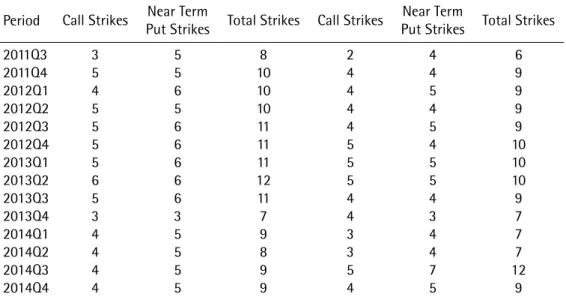
The market of options over Ibovespa presents a low liquidity. The average daily volume traded in this market is about US$20 million (about 1.5% of the daily volume of options over S&P 500 traded in the US). As a consequence, we have few strikes to work with. On average, 10 different strikes for the near-term and 10 different strikes for the next-term, considering both calls and puts.Table 1reports the quarterly daily averages of the number of strikes that we use.8
Table 1.NUMBER OF OPTION STRIKES USED IN THEIVOL-BR
The table shows the quarterly daily averages of the number of strikes that were used in the construction of the IVol-BR.
Period Call Strikes Put StrikesNear Term Total Strikes Call Strikes Put StrikesNear Term Total Strikes
2011Q3 3 5 8 2 4 6
2011Q4 5 5 10 4 4 9
2012Q1 4 6 10 4 5 9
2012Q2 5 5 10 4 4 9
2012Q3 5 6 11 4 5 9
2012Q4 5 6 11 5 4 10
2013Q1 5 6 11 5 5 10
2013Q2 6 6 12 5 5 10
2013Q3 5 6 11 4 4 9
2013Q4 3 3 7 4 3 7
2014Q1 4 5 9 3 4 7
2014Q2 4 5 8 3 4 7
2014Q3 4 5 9 5 7 12
2014Q4 4 5 9 4 5 9
The methodology presented above departs from the standard one described inCarr & Wu(2009) for three reasons which are related to the relatively low liquidity and low number of strikes traded in the options market in Brazil:
1) We introduce the adjustment factorj in equation (1) to account for the following: (i) there are
days when only a call or a put atK0 is traded—Carr & Wu(2006) have always both a call and a put—; moreover, (ii) we have to defineK0as the option strike value which is closest toF(t,Tk) and, because of that, we may have eitherK0>F(t,Tk)orK0<F(t,Tk)—Carr & Wu(2006) define
K0 as the option strike value immediately belowF(t,Tk). Depending on the situation we face regarding (i) and (ii), the value ofj is set to0,1 2, as follows (an explanation about this can be found in theAppendix):
Table 2.POSSIBLE VALUES OFj
K0<F K0>F K+0=F
∃call,∃put 1 1 1
∃call,∄put 2 0 0
∄call,∃put 0 2 0
2) We widen the time frame of options prices to the interval [3 pm, 6 pm]. For each strike, we use the last deal in this interval to synchronize the option price with the settlement price of the Ibovespa futures;
3) We only calculateσ12(t)andσ22(t)if, for each vertex, there are at least 2 trades involving OTM call
options at different strikes and 2 trades involving OTM put options also at different strikes—this is done in order to avoid errors associated with lack of liquidity in the options market. If on a given day only one volatility vertex can be calculated, we suppose that the volatility surface is flat and the IVol-Br is set equal to the computed vertex. If both near- and next-term volatilities cannot be calculated, we report the index for that day as missing.
The volatility index calculated according to equations (1) and (2) could be biased because it con-siders only traded options at a finite and often small number of strikes. To assess the possible loss in the accuracy of the integral calculated with a small number of points, we refine the grid of options via a linear interpolation using 2,000 points of the volatility smile that can be obtained from the traded options (based on the procedure suggested byCarr & Wu,2009).9 The results did not change.
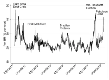
The IVol-BR series, computed according to the methodology described above, is available for down-load at the webpage of the Brazilian Center for Research in Financial Economics of the University of Sao Paulo (NEFIN).10Figure 1plots the IVol-Br for the period between August 2011 and February 2015, com-prising 804 daily observations.
Figure 1.IMPLIED VOLATILITY INBRAZIL – THEIVOL-BR
This figure shows the daily time-series of the IVol-Br in percentage points and annualized.
9The “coarse” volatility smile for both near and next-term is retrieved from the options market values and the Black-76 formula. We then refine the grid of strike pricesKiusing the implied volatilities and implied deltas of the options with the formula:
Ki=F(t,T)exp
[
−wσi√T−t N−1(∆i+12σi2(T−t)
)] ,
wherew=1for calls andw=−1for puts;N−1(·)is the inverse of the standard normal cumulative density function. To simplify the process of retrievingKi , we transform all traded options in calls (via put-call parity) and create a smile in the
([∆call,σ)space. We then generate 2,000 points by linearly interpolating this smile considering two intervals: (i) the interval ∆max;∆min]of deltas of the traded options; (ii) the interval[99; 1]of deltas.
An implied volatility index should reflect the dynamics of (i) the level, or quantity, of risk that investors face—the expected future volatility—and (ii) the price of such risk—the risk-aversion of in-vestors. Given that, the IVol-BR should be higher in periods of distress. As expected, asFigure 1shows, the series spikes around events that caused financial distress in Brazil, such as the Euro Area debt crisis (2011), the meltdown of oil company OGX (2012), the Brazilian protests of 2013, the second election of Mrs. Rousseff (2014) and the corruption and financial crisis in Petrobras (2015).
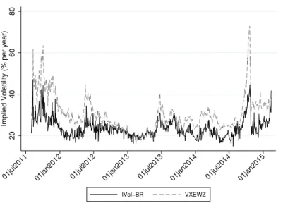
It is also interesting to compare the IVol-BR with the VXEWZ, the CBOE’s index that tracks the implied volatility of a dollar-denominated index (EWZ) of the Brazilian stock market.Figure 2shows the evolution of both series.
AsFigure 2presents, the VXEWZ is often higher than IVol-BR. This happens because the VXEWZ, which is constructed using options over the EWZ index (that tracks the level in dollars of the Brazilian stock market), embeds directly the exchange rate volatility. In turn, the IVol-BR is constructed using options over the Ibovespa itself and, hence, reflects only the stock market volatility. Thus the IVol-BR is better suited to describe the implied volatility of the Brazilian stock market for local investors or foreign investors that have hedged away the currency risk. During the period depicted inFigure 2there were important changes in the exchange rate volatility that directly impacted the VXEWZ but not the IVol-BR.
Figure 2.COMPARINGIVOL-BRANDVXEWZ
This figure shows the daily time-series of the IVol-Br and the VXEWZ. Both series are in percentage points and annualized. VXEWZ is the implied volatility index on the Brazilian stocks ETF EWZ and is calculated by CBOE.
20
40
60
80
Implied Volatility (% per year)
01jul2011 01jan2012 01jul2012 01jan2013 01jul2013 01jan2014 01jul2014 01jan2015
IVol−BR VXEWZ
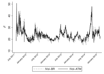
2.1. Comparison of IVol-BR with ATM volatility
As can be seen inFigure 3, both Ivol-BR and Ivol-ATM series are highly correlated (0.92). This is not surprising, since a similar pattern is also observed between the VIX and the VXO, the Black-Scholes implied volatility version of the VIX that also uses only only at-the-money options on the S&P 500 index. Indeed, both VIX and VXO have a correlation of 0.99 during the same sample period.11
InCarr & Wu(2006) we can find a discussion on the reasons which led to the adoption of the VIX. Firstly, the VIX is model-free and the VXO depends on the Black-Scholes framework. Secondly, although both VIX and VXO provide good approximations of the volatility swap rate, the VIX is much easier to replicate using option contracts than the VXO. Indeed, despite its popularity as a general volatility reference index, no derivative products have been launched on the VXO index. In contrast, less than a year after its introduction, the VIX was already serving as basis for new futures contracts.
Figure 3.COMPARINGIVOL-BRANDVXEWZ
This figure shows the daily time-series of the IVol-Br and the IVol-ATM. Both series are in percentage points and annualized. IVol-ATM is the Black-Scholes implied volatility calculated using only at-the-money options.
10
20
30
40
50
%
July 2011 January 2012
July 2012 January 2013
July 2013 January 2014
July 2014 January 2015
IVol−BR IVol−ATM
3. EMPIRICAL ANALYSIS USING THE IVOL-BR
In this section we use the squared IVol-BR series, which we call IVar, in some interesting empirical ex-ercises. We first decompose the IVar into (i) the actual expected variance of stock returns and (ii) the variance premium.12 Then, from the variance premium, we produce a time-varying risk-aversion mea-sure for the Brazilian investor. Finally, we show empirically that higher risk-aversion is accompanied with higher expected returns, as asset pricing theory suggests. The reason for working with the IVar, instead of the IVol-BR, is that theoretical models usually produce closed-form equations that relate risk aversion to the variance premium and not the volatility premium.
11Prior to September 2003 the Chicago Board of Options Exchange (CBOE) calculated a volatility index that used only ATM options. However, even after introducing the new VIX, the CBOE continued to calculate the older, ATM index, under a new name (VXO). Both data sets can be downloaded from the CBOE website.
12It can be shown that the implied variance approximates the expected variance under the risk neutral measure (see for instance
Insection 3.1we decompose the implied variance, calculated as the IVol-BR squared, into (i) the expected variance of stock returns and (ii) the equity variance premium. To do this, we first estimate a model that represents the conditional expectation of investors of future variance. Then, by calculating the difference between the implied variance and the estimated expected variance, we arrive at a daily measure of the variance premium. Insection 3.2, from the volatility premium, we produce a time-varying risk aversion measure for the Brazilian investor from the variance premium. Insection 3.3we show that the variance premium and the risk aversion measure are able to predict future stock returns as theory suggests: when variance premium (risk-aversion) is higher, expected returns are higher.
3.1. Decomposing implied variance into expected variance and variance premium
To decompose implied variance into expected variance and a premium, we first search for the model that best forecasts variance. Because the implied variance, calculated by squaring the IVol-BR, reflects markets expectations for the two-months ahead, the measure of expected variance of interest is also over the same two-month period.
The variance of returns is a latent, unobservable variable. Fortunately, we can obtain a good estimator of the variance of returns from high frequency data and use the estimated time-series, the so-called realized variance, as the dependent variable of our forecasting model. Formally, the realized variance over a two-month period at daytis calculated by summing squared 5-minute returns over the last 42 trading days:
RVt(42)=252 42 ×
⌊42∑/∆⌉
i=1
ri2,
where∆=5/425is the 5-minute fraction of a full trading day with 7 hours including the opening observa-tion;⌊·⌉is the operator that approximates to the closest integer; andri=100×[ln(Ibovi)−ln(Ibovi
−i) ]
is a 5-minute log-return in percentage form on the Ibovespa index, except whenirefers to the first price
of the day, in which caseri corresponds to the opening/close log-return.
Following the recent literature on variance forecasting (Chen & Ghysels,2011,Corsi,2009,Corsi & Renò,2012, andBekaert & Hoerova,2014), we construct several explanatory variables (predictors) from a 5-minute returns data set.13First, we include in the set of explanatory variables lags of realized variance at heterogeneous frequencies to account for the clustering feature of stock returns variance. In the spirit of Corsi’s HAR model (Corsi,2009), lags of bimonthly, monthly, weekly and daily realized variances are included: RV(42)
t ,RV
(21)
t ,RV
(5)
t andRV
(1)
t . Formally:
RV(k)
t = 252
k ×
⌊∑k/∆⌉
i=1
ri2
for eachk=42,21,5,1.
One important feature of variance is the asymmetric response to positive and negative returns, commonly referred to as leverage effect. To take this into account,Corsi & Renò(2012) suggests including lags of the following “leverage” explanatory variables:
Lev(k)
t =− 42
k
⌊∑k/∆⌉
i=1
min{ri,0},
withk=42,21,5,1. For a convenient interpretation of the estimated parameters, we take the absolute value of the cumulative negative returns.
Andersen, Bollerslev, & Diebold(2007) show that jumps help in predicting variance. Following the theory laid out byBarndorff-Nielsen & Shephard(2004), realized variance can be decomposed into its continuous and jump components with the usage of the so-called bipower variation (BPV). As shown by these authors, under mild conditions, the BPV is robust to jumps in prices while the realized variance is not. This insight allows one to identify jumps indirectly by simply calculating the difference:
Jt=max{RVt−BPVt,0},
whereBPVt =252
42 ×
∑⌊42/∆⌉
i=1 |ri||ri−1|. The maximum operator is included to account for the situation when there are no jumps and the BPV is eventually higher than the realized variance. The continuous component of the realized variance is defined as follows:
Ct=RVt−Jt.
Lagged variables of the continuous and jump components at other time frequencies are also in-cluded. Using the same notation as before, the following eight variables are addedCt(k),Jt(k)withk=42, 21,5,1.
Finally, we followBekaert & Hoerova(2014) and include the lagged implied variance as explanatory variable. Importantly, as will be shown, this variable contains information about future realized variance that is not contained in lagged realized variance and other measures based on observed stock returns.
To find the best forecasting model, we apply the General-to-Specific (GETS) selection method pro-posed by David Hendry (see for instanceHendry, Castle, & Shephard,2009). The starting model, also called GUM or General Unrestricted Model, includes all the variables described above plus a constant:
RVt+42=c+γ1IVart+γ2C(42)
t +γ3C
(21)
t +γ4C
(5)
t +γ5C
(1)
t +γ6J
(42)
t +γ7J
(21)
t +γ8J
(5)
t +γ9J
(1)
t
+γ10Levt(42)+γ11Lev
(21)
t +γ12Lev
(5)
t +γ13Lev
(1)
t +ϵt. To avoid multicolinearity, the lagged realized variance measures were excluded from the initial set of ex-planatory variables since by construction they are approximately equal toRV(k)
t ≈C
(k)
t +J
(k)
t . However, in a robustness exercise below, we include these variables in other forecasting models.
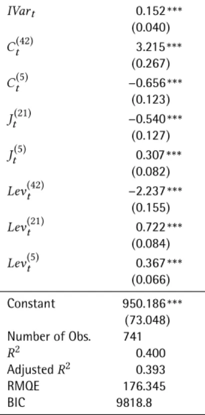
Following an iterative process, the method searches for variables that improve the fit of the model but penalizes for variables with statistically insignificant parameters. The regressions are based on daily observations.Table 3shows the estimates of the final model—the GETS model. Eight variables plus a constant remain in the GETS model:IVart,C(42)
t ,C
(5)
t ,J
(21)
t ,J
(5)
t ,Lev
(42)
t ,Lev
(21)
t andLev
(5)
t .
Importantly, the coefficient on the implied variance is positive (0.152) and highly significant. This indicates that, as expected, IVar does contain relevant information about future variance, even after controlling for traditional variance forecasting variables.
From the GETS model, we calculate a time-series of expected variance. We name the difference between implied variance and this time-series of expected variance as the variance premium:
VariancePremiumt=IVart−Dσt2, (3)
whereDσt2=Et [
RVt+42]=Et [
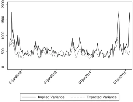
σt2,t+42]is the GETS model expected variance computed using information up until dayt; the subscriptt+42emphasizes the fact that it is the expected variance over the same horizon as the implied variance, IVart. Figure 4shows both series andFigure 5shows the variance
Figure 4.IMPLIED VARIANCE AND EXPECTED VARIANCE
This figure shows the weekly time-series of the implied variance—the squared of the IVol-Br—and the estimated
expected variance. The model for expected volatility is the GETS model shown onTable 3. Both series are in
percentage points and annualized.
0
500
1000
1500
2000
01jan2012 01jan2013 01jan2014 01jan2015
data
Implied Variance Expected Variance
Figure 5.THE VARIANCE PREMIUM
This figure shows the weekly time-series of the variance premium calculated by the difference of the implied
variance and expected variance as predicted by the GETS model shown onTable 3, and its three month moving
average.
−50
0
50
100
01jan2012 01jan2013 01jan2014 01jan2015
data
Table 3.GENERAL-TO-SPECIFIC BEST MODEL
The table shows the estimates of the best variance forecasting model following the General-to-Specific selection method. The starting model, also called GUM or General Unrestricted Model, comprises of all independent vari-ables. The standard errors reported in parenthesis are robust to heteroskedasticity. Regressions are based on daily observations. The correspondingp-values are denoted by * ifp<0.10, **ifp<0.05and***ifp<0.01.
IVart 0.152***
(0.040)
Ct(42) 3.215***
(0.267)
Ct(5) −0.656***
(0.123)
Jt(21) −0.540***
(0.127)
Jt(5) 0.307***
(0.082)
Lev(42)
t −2.237***
(0.155)
Lev(21)
t 0.722***
(0.084)
Lev(5)
t 0.367***
(0.066)
Constant 950.186***
(73.048)
Number of Obs. 741
R2 0.400
AdjustedR2 0.393
RMQE 176.345
BIC 9818.8
3.2. The variance risk premium and the risk aversion coefficient
An implied variance index reflects the dynamics of two very important variables. The first relates to the level, or quantity, of risk that investors face: the expected future variance of the market portfolio, estimated above. The second relates to the price of such risk: the risk aversion of the representative investor.
Since options’ payoffs are asymmetric, the value of any option (call or put) is increasing in the expected variance of the underlying asset. Because of that, options are often used as a protection against changes in expected variance. Since the typical risk-averse investor dislikes variance, options are traded with a premium because of such an insurance value. As a direct consequence, the implied variance (IVar, the IVol-BR squared), which is computed directly from options prices, also has a premium with respect to the expected variance. That is, the more risk-averse the investor is, the more she is willing to pay for the insurance that options provide, i.e., the higher the variance premium.
closed-form equation for the variance premium holds for eacht:14
VariancePremiumt =ψ
−1 −γt 1−ψ−1 ×
κ1(1−γt)2
2( 1−γt 1−ψ−1
) (
1−κ1ρσ)
q, (4)
whereψis the coefficient of elasticity of intertemporal substitution,γtis the time-varying risk aversion coefficient,q the volatility of the volatility, andρσ is the auto-regressive parameter in the volatility of
consumption.
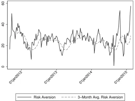
Using the estimated weekly series for the variance premium computed above and usual parameter calibration,15we pin down a time-series for the time varying risk aversion coefficient of the represen-tative investor in Brazil.16 The resulting series is plotted inFigure 6. The smallest value forγt is 1 on August 22, 2014; and the highest value is 57 on February 13, 2015. The average risk aversion level is 26. Such values are consistent with the results inZhou(2009)—an average risk aversion higher than 10 is needed to match the empirical moments of the variance premium (see his Table 8).
Figure 6.RISK AVERSION
This figure show a time-series for the risk aversion index in Brazil. It is computed by combining the weekly series
for the variance premium withBollerslev et al.(2009) functional form for the variance premium, as explained in
section 3.3.
0
20
40
60
01jan2012 01jan2013 01jan2014 01jan2015
data
Risk Aversion 3−Month Avg. Risk Aversion
Using different methodology and data sets, other papers find (unconditional) lower estimates of risk aversion for the Brazilian representative investor. For instance,Fajardo, Ornelas, & Farias(2012) using data on currency options for the Brazilian Real from 1999 to 2011, estimate the implied risk-neutral density and, by comparing it to the objective density, find a coefficient of relative risk aversion of around 2.7. Similarly,Issler & Piqueira(2000) using data on aggregate consumption from 1975 to 1994,
14We use their simpler equation, where they assume a constant volatility of volatility (the processqis constant at allt).
15We setψ
=1.5,q=10−6,κ
1=0.9andρσ =0.978following the calibration inBansal & Yaron(2004) andBollerslev et al. (2009).
document a coefficient of relative risk aversion lower than five. In the next section we assess to which extent the lower risk aversion found in other studies can be attributed to differences in calibration.
3.2.1. Sensitivity of risk-aversion to calibration parameters
A number of papers estimate the elasticity of intertemporal substitution for the Brazilian representative investor. Issler & Piqueira(2000) find a relatively lowψ of 0.29 using annual consumption data from 1975 to 1994—less than half of theψ they find for the US (0.72) for the same period and using the same methodology. A low value ofψ for the Brazilian economy is also reported byHavranek, Horvath, Irsova, & Rusnak(2015); the authors find that households in developing countries and countries with low stock market participation, such as Brazil, substitute a lower fraction of consumption intertemporally in response to changes in expected asset returns, with implied values forψ often below one. On the other hand, using a quarterly data set of 1975 to 2000,Araújo(2005) finds a much higher range of possible ψ’s, with the minimum value ofψ being equal to 2.5. Given that there is no consensus on which is the ψ that best characterize the behavior of the representative investor in Brazil, we assess the sensitivity of our results to the choice ofψ by comparing the estimates ofγt for three different values ofψ: 0.50, 1.50, and 3.00.
Another parameter that was used in the calibration that can vary across countries isκ1. The parameterκ1 is equal to the ratioPD/(1+PD), wherePDis a long-run average of the price-dividend ratio. The number used in our calibration was 0.9 and is the same one used Bollerslev et al.(2009). According to its formula, the value ofκ1=0.9corresponds to a price-dividend ratio of around 10. This number, however, can vary depending on the data set considered. Indeed, the average price-dividend ratio computed for Brazil in the period 2001–2015 is around 40. Thus, we also assess the sensitivity of our results to the choice ofκ1by comparing the estimates ofγt for another two different values ofκ1: 0.98 and 0.95. These two values correspond, respectively, to price-dividend ratios of 40 and 20.
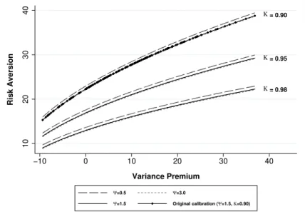
Figure 7shows the image of the functionγt—the inverse of the function in equation (4)—for plausible values of the variance premium and for nine pairs of(
ψ,κ1), each one a possible combination
Figure 7.RISK AVERSION AS A FUNCTION OFψ ANDκ1
This figure shows the image of theγt function for reasonable values of the variance premium and for different
choices ofψ andκ1.
Κ= 0.90
Κ= 0.95
Κ= 0.98
10
20
30
40
Risk Aversion
−10 0 10 20 30 40
Variance Premium
Ψ=0.5 Ψ=3.0
ofψ =(0.5,1.5,3.0) with κ1=(0.90,0.95,0.98). The estimated values ofγt differ depending on the chosen parametrization, particularly acrossκ1. At a variance premium of five,γt can be 13, 16, or 23 ifκ1 is, respectively, 0.98, 0.95, or 0.90. On the other hand, the values ofγt do not vary much across ψ; for any givenκ1and value of variance premium, the range of possible values forγt is less than one. Overall, at any pair of (
ψ,κ1) considered the estimates ofγt are higher than 10.
3.3. Predicting future returns
If the variance premium positively comoves with investors risk-aversion, it should predict future market returns: when risk aversion is high, prices are low; consequentially, future returns (after risk aversion reverts to its mean) should be high. Moreover, the risk aversion measure itself, computed insection 3.2, should also predict future returns. In this Section we test these predictions by regressing future market returns on both the variance premium and the risk-aversion measure.
Table 4shows the results of our main regression. The dependent variable is the return on the market portfolio 4 weeks ahead. To limit the overlapping of time-series, we reduce the frequency of our data set from daily to weekly by keeping only the last observation of the week. Additionally, to account for the remaining serial correlation in the error term, the standard errors are computed using Newey-West estimator. Columns (1) and (2) show that implied variance IVart and expected variance
D
σt2alone are not very good predictors of future returns. On the other hand, Column (3) shows that the variance premium, resulting from a combination of both variables,IVart−Dσt2, strongly predicts future
returns at the 4-week horizon. The estimated coefficient is positive, 0.089, and significant at the 1%
confidence level. Column (4) shows that the risk aversion measure also predicts future returns at the 4-week horizon. The estimated coefficient is positive, 0.180, and significant at the 1% confidence level. The predictive power of the variance premium and the risk aversion measure remains after we include in the regression the divided yield log(Dt/Pt), another common predicting variable. Again, columns (5) and (6) show that implied variance and expected variance alone are poor predictors of returns. On the other hand, both the variance premium and the risk aversion measure do predict future returns. Column (7) shows a positive coefficient for the variance premium, 0.066, significant at the 5% confidence level. Column (8) shows a positive coefficient for the risk-aversion measure, 0.135, also significant at the 5% confidence level.
In columns (1) through (8) of tables5and6, the regressions are the same as the one in Column (7) and (8), respectively, ofTable 4, except for the horizon of future returns. As the significance and values of the estimates indicate, the variance premium predictability is stronger at the 4-week horizon—columns (7) and (8).
A concern is that the standard errors in the first eight Columns in tables5and6may be biased due to the presence of a persistent explanatory variable such as the log dividend yield (see for instance Stambaugh,1999) combined with a persistent dependent variable (overlapping returns). To address this concern, columns (9) and (10) in both tables show the same regressions of columns (7) and (8) but based onnon-overlapping4-week returns. As we can see, the coefficients on the variance premium and risk-aversion remain positive and significant.
Another concern may be that the actual expected variance by market participants cannot be ob-served. Hence, our measure of expected variance depends on the model chosen by the econometrician. To address this concern, we also assess to which extent our results depend on the chosen variance model. Tables7and8show the estimates of several models. Table7brings the estimates of Corsi’s HAR model (Corsi,2009) in Column (1), with the addition of a 42-day realized variance lag in accordance with the frequency of the dependent variable. In columns (2), (3) and (4) we include the lagged implied vari-ance, IVart, that was shown to contain important predictive information. Columns (3) and (4) include
,F
.Chague,
B.
Giovannetti
and
M.E.
da
Silva
Table 4.PREDICTABILITY REGRESSIONS
The table shows the estimates of predictability regressions. The dependent variable is the return on the market portfolio 4-weeks ahead. The explanatory variables
are: i)Dσ2
t, the expected variance on the next 8 weeks estimated by best model following the General-to-Specific selection method; ii)IV art, the expected implied
variance on the next 8 weeks estimated from prices of options contracts at timet; iii)IVart−Dσ2
t, the variance premium; iv)γt is the risk aversion computed using
the functional form inBollerslev et al.(2009) and the variance premium; and v)log(Dt/Pt), the log dividend yield. Regressions are based on weekly observations. To
account for error correlation, the standard errors are computed using Newey-West lags. The standard errors are reported in parenthesis. The correspondingp-values
are denoted by *ifp<0.10, **ifp<0.05and***ifp<0.01.
4 weeks
(1) (2) (3) (4) (5) (6) (7) (8)
D
σt2 0.000 −0.002
(0.005) (0.004)
IVart 0.004* 0.002
(0.002) (0.002)
IVart−Dσ2
t 0.089*** 0.066**
(0.032) (0.031)
γt 0.180*** 0.135**
(0.057) (0.059)
log(D/P) 14.928*** 12.684*** 11.449*** 11.303***
(5.482) (6.169) (6.157) (6.132)
Constant 0.589 −1.854 −0.314 −4.228*** 47.919*** 38.601* 35.594* 32.204 (2.349) (1.345) (0.579) (1.538) (17.131) (19.719) (19.315) (19.956)
Number of Obs. 175 175 175 175 175 175 175 175
R2 0.000 0.044 0.082 0.086 0.096 0.108 0.135 0.137
AdjustedR2 −0.001 0.038 0.077 0.081 0.086 0.098 0.125 0.127
de
Janeiro
v.
71
n.
1
/p.
3
–
28
Jan-Mar
Variance
pr
emium
and
implied
volatility
in
a
low-liquidity
option
mark
et
i) t−Dσt is theex-antevolatility premium; and ii)log Dt/Pt is the log dividend yield. Regressions in columns (1) through (8) are based on weekly
obser-vations. Regressions in columns (9) and (10) are non-overlapping on the dependent variable and are based on monthly obserobser-vations. To account for error correlation,
standard errors in columns (3) through (8) are computed using Newey-West lags. The standard errors reported in parenthesis. The correspondingp-values are denoted
by * ifp<0.10, **ifp<0.05and***ifp<0.01.
1 week 2 weeks 3 weeks 4 weeks 3 weeks N-O
(1) (2) (3) (4) (5) (6) (7) (8) (9) (10)
IVart−Dσ2
t 0.028* 0.023 0.038* 0.026 0.059* 0.043 0.089** 0.066* 0.136** 0.112*
(0.017) (0.018) (0.021) (0.020) (0.030) (0.028) (0.032) (0.031) (0.050) (0.063)
log(D/P) 3.067 6.102* 7.939 11.449* 6.032
(2.399) (3.571) (5.385) (6.157) (9.099)
Constant −0.129 9.487 −0.095 19.042* −0.191 24.707 −0.314 35.594* −0.431 18.508 (0.208) (7.559) (0.338) (11.188) (0.462) (16.933) (0.579) (19.315) (0.730) (28.585)
Number of Obs. 178 178 177 177 176 176 175 175 41 41
R2 0.033 0.047 0.028 0.056 0.047 0.079 0.082 0.135 0.135 0.149 AdjustedR2 0.028 0.036 0.023 0.045 0.041 0.067 0.077 0.125 0.113 0.104
RBE
Rio
de
Janeiro
v.
71
n.
1
/p.
3
–
28
Jan-Mar
,F
.Chague,
B.
Giovannetti
and
M.E.
da
Silva
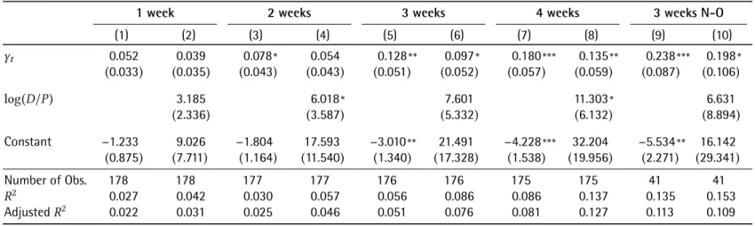
Table 6.PREDICTABILITY REGRESSIONS AT DIFFERENT HORIZONS WITH RISK AVERSION
The table shows regressions having future market returns 1-week ahead, 2-, 3- and 4-weeks ahead as the dependent variable. The explanatory variables are: i)γt
is the risk aversion computed using the functional form inBollerslev et al.(2009); and ii)log(Dt/Pt) is the log dividend yield. Regressions in columns (1) through
(8) are based on weekly observations. Regressions in columns (9) and (10) are non-overlapping on the dependent variable and are based on monthly observations. To account for error correlation, standard errors in columns (3) through (8) are computed using Newey-West lags. The standard errors reported in parenthesis. The
correspondingp-values are denoted by * ifp<0.10,**ifp<0.05and***ifp<0.01.
1 week 2 weeks 3 weeks 4 weeks 3 weeks N-O
(1) (2) (3) (4) (5) (6) (7) (8) (9) (10)
γt 0.052 0.039 0.078* 0.054 0.128** 0.097* 0.180*** 0.135** 0.238*** 0.198*
(0.033) (0.035) (0.043) (0.043) (0.051) (0.052) (0.057) (0.059) (0.087) (0.106)
log(D/P) 3.185 6.018* 7.601 11.303* 6.631
(2.336) (3.587) (5.332) (6.132) (8.894)
Constant −1.233 9.026 −1.804 17.593 −3.010** 21.491 −4.228*** 32.204 −5.534** 16.142 (0.875) (7.711) (1.164) (11.540) (1.340) (17.328) (1.538) (19.956) (2.271) (29.341)
Number of Obs. 178 178 177 177 176 176 175 175 41 41
R2 0.027 0.042 0.030 0.057 0.056 0.086 0.086 0.137 0.135 0.153 AdjustedR2 0.022 0.031 0.025 0.046 0.051 0.076 0.081 0.127 0.113 0.109
de
Janeiro
v.
71
n.
1
/p.
3
–
28
Jan-Mar
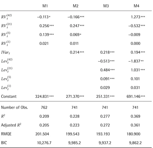
Table 7.ROBUSTNESS:DIFFERENT VARIANCE MODELS
The table shows the estimates of different models of expected variance. The dependent variable is the realized variance over the following 42 days, calculated from 5-minute returns on the Ibovespa portfolio. The explanatory
variables are: i)IVart is the expected implied variance on the next 8 weeks estimated from prices of options
contracts at timet−1; ii)RV(k)
t−1 is the realized volatility on the followingk days at timet−1, wherek=42,
21,5,1; computed iii)Lev(k)
t−1is the cumulative negative 5-minute returns continuous component of the realized
variance on the followingkdays at timet−1, wherek=42,21,5,1. The standard errors reported in parenthesis.
The correspondingp-values are denoted by * ifp<0.10, **ifp<0.05and***ifp<0.01.
M1 M2 M3 M4
RV(42)
t −0.113* −0.166*** 1.273***
RV(21)
t 0.256*** 0.247*** −0.532***
RV(5)
t 0.139*** 0.069* −0.009
RV(1)
t 0.021 0.011 0.000
IVart 0.214*** 0.218*** 0.194***
Lev(42)
t −0.513*** −1.837**
Levt(21) 0.484*** 1.031***
Lev(5)
t 0.091*** 0.101
Levt(1) 0.029 0.031
Constant 324.831*** 271.370*** 251.331*** 691.146***
Number of Obs. 762 741 741 741
R2 0.209 0.228 0.277 0.369
AdjustedR2 0.205 0.223 0.272 0.361
RMQE 201.504 199.543 193.193 180.900
Table 8.ROBUSTNESS:DIFFERENT VARIANCE MODELS (CONT.)
The table shows the estimates of different models of expected realized variance. The dependent variable is the realized variance over the following 8-weeks, calculated from 5-minute returns on the Ibovespa portfolio. The
explanatory variables are: i)IVart
−1is the expected implied variance on the next 8 weeks estimated from prices
of options contracts at timet−1; ii) Ct(k−)1 is the continuous component of the realized variance during the
followingk days at timet−1, wherek=42,21,5,1; iii)Jt(k−)1is the jump component of the realized variance
during the followingk days at timet−1, wherek =42,21,5,1; and iv)Levt(k−)1 is the absolute of the sum
5-minute negative returns during the followingkdays at timet−1, wherek=42,21,5,1. The standard errors
reported in parenthesis. The regressions are based on daily observations. The correspondingp-values are denoted
by * ifp<0.10,**ifp<0.05and***ifp<0.01.
M5 M6 M7 M8
IVart−1 0.147*** 0.142*** 0.286***
Ct(42−1) 3.282*** 3.679*** −1.675***
Ct(21−1) −0.514 −1.171*** 1.545***
Ct(5−)1 −0.461*** −0.225* 0.010
Ct(1−)1 −0.057 −0.025 −0.015
Jt(−421) 0.294 1.583*** 1.308***
Jt(−211) −0.540** −0.768*** −1.126***
Jt(−5)1 0.247*** 0.052 0.163
Jt(−1)1 0.021 0.007 0.026
Lev(42)
t−1 −2.433*** −2.535*** −1.289***
Lev(21)
t−1 1.023*** 1.178*** 0.802***
Lev(5)
t−1 0.263*** 0.211*** 0.077
Lev(1)
t−1 0.043 0.043 0.021
IVolt
−1 13.969***
Constant 930.537*** 935.469*** 337.173*** 256.965***
Number of Obs. 741 741 741 741
R2 0.406 0.397 0.349 0.269
AdjustedR2 0.396 0.390 0.341 0.260
RMQE 175.994 176.881 183.726 194.766
InTable 8we separate the realized variance into its continuous and jump components and use these variables instead. Column (1) shows the estimates of the GUM model, the starting model in the General-to-Specific selection method adopted in section3.1. The GUM regression includes all the vari-ables initially selected as candidate varivari-ables to forecast variance. Columns (2) through (4) are variants of this more general model.
As we can conclude by comparing the statistical properties of each regression in tables3,7and8, the GETS model has the lowest information criterion, BIC, as the selection method strongly penalizes the inclusion of variables and favors a more parsimonious model. Models M4, M5 and M6 have comparable
R2 to the GETS models, explaining more than 35% of the variation of the dependent variable, but with the inclusion of extra regressors.
We now assess how sensitive is our predictive regression to the selection of the variance model. For each one of the regression models shown in tables7and8we calculate a volatility premium as in equation (3). The results of the predictability regressions at the 4-week return horizon are shown in Table 9. In Column (1) we use a simple model to predict future variance and setDσt2=σt2−1 following the definition ofBollerslev et al.(2009). Column (2) replicates our main regression that uses the GETS model to predict variance. Columns (3) through (10) show the predictability regressions for each of the 8 models presented in tables7and8. As can be seen, the results are largely robust to the selection of the variance model.
4. CONCLUSION
This is the first article to propose an implied volatility index for the Brazilian stock market based on option and futures prices traded locally. The methodology we propose has to deal with the relatively low liquidity of contracts used. This is a first contribution of this paper.
We use our implied volatility index to calculate the so-called variance premium for Brazil. Assum-ingBollerslev et al.(2009) economic structure, we also pin down a time-varying risk aversion measure of the representative investor in the Brazilian market. In line with international evidence, we show the variance premium strongly predicts future stock returns. Interestingly, we also find that our measure of risk aversion is a strong predictor of future returns with a slightly superior fit than the variance pre-mium. To the best of our knowledge, this is the first analysis of this kind for an emerging market. This is the second contribution of this paper.
,F.
Chague,
B.
Giovannetti
and
M.E.
da
Silva
premium as regressors. Each measure of variance premium is calculated with a different model for expected variance. Column (1) uses a simple model for expected
variance:Dσ2
t =σt2−42, and was proposed byBollerslev et al.(2009). Column (2) replicates our main regression that uses the GETS model to forecast variance. Columns
(3) through (10) varies the expected variance model from M1 to M10.log(Dt/Pt)is the log dividend yield. Regressions are based on weekly observations. To account
for error correlation, the standard errors are computed using Newey-West lags. The standard errors are reported in parenthesis. The correspondingp-values are
denoted by *ifp<0.10, **ifp<0.05and ***ifp<0.01.
(1) GETS(2) (3) (4) (5) (6) (7) (8) (9) (10)
Constant 50.656*** 35.594* 37.988** 38.108** 37.454* 33.082* 34.887* 34.788* 33.337* 37.230*
(17.423) (19.315) (18.852) (19.122) (19.386) (19.675) (19.394) (19.569) (19.601) (19.185) log(D/P) 16.234*** 11.449* 12.188** 12.235** 12.007* 10.675* 11.233* 11.201* 10.751* 11.964* (5.583) (6.157) (6.021) (6.098) (6.179) (6.268) (6.181) (6.235) (6.245) (6.114)
IVart−σ2
t−1 0.005***
(0.002)
IVart−Dσt2 0.007**
(0.003)
IVart−Dσ2
t(M1) 0.005**
(0.002)
IVart−Dσ2
t(M2) 0.005*
(0.003)
IVart−Dσ2
t(M3) 0.004*
(0.002)
IVart−Dσ2
t(M4) 0.006**
(0.003)
IVart−Dσ2
t(M5) 0.006**
(0.003)
IVart−Dσ2
t(M6) 0.006**
(0.003)
IVart−Dσ2
t(M7) 0.006**
(0.003)
IVart−Dσ2
t(M8) 0.005**
(0.003)
Number of Obs. 175 175 175 175 175 175 175 175 175 175
R2 0.015 0.135 0.127 0.119 0.114 0.147 0.140 0.138 0.143 0.126
AdjustedR2 0.140 0.125 0.116 0.109 0.104 0.137 0.130 0.128 0.133 0.116
de
Janeiro
v.
71
n.
1
/p.
3
–
28
Jan-Mar
REFERENCES
Andersen, T. G., Bollerslev, T., & Diebold, F. X. (2007). Roughing it up: Including jump components in the
measure-ment, modeling, and forecasting of return volatility. Review of Economics and Statistics,89(4), 701–720.
doi:10.1162/rest.89.4.701
Araújo, E. (2005). Avaliando três especificações para o fator de desconto estocástico através da fronteira de
volatil-idade de Hansen e Jagannathan: Um estudo empírico para o Brasil.Pesquisa e Planejamento Econômico,
35(1). Retrieved fromhttp://repositorio.ipea.gov.br/handle/11058/4395
Bansal, R., & Yaron, A. (2004). Risks for the long run: A potential resolution of asset pricing puzzles.The Journal
of Finance,59(4), 1481–1509. doi:10.1111/j.1540-6261.2004.00670.x
Barndorff-Nielsen, O. E., & Shephard, N. (2004). Power and bipower variation with stochastic volatility and jumps. Journal of Financial Econometrics,2(1), 1–37. doi:10.1093/jjfinec/nbh001
Bekaert, G., & Hoerova, M. (2014). The VIX, the variance premium and stock market volatility.Journal of
Econo-metrics,183(2), 181–192. doi:10.1016/j.jeconom.2014.05.008
Bollerslev, T., Gibson, M., & Zhou, H. (2011). Dynamic estimation of volatility risk premia and investor risk
aversion from option-implied and realized volatilities. Journal of Econometrics, 160(1), 235–245. doi:
10.1016/j.jeconom.2010.03.033
Bollerslev, T., Marrone, J., Xu, L., & Zhou, H. (2014). Stock return predictability and variance risk premia: Statistical
inference and international evidence. Journal of Financial and Quantitative Analysis,49(3), 1–50. doi:
10.1017/S0022109014000453
Bollerslev, T., Tauchen, G., & Zhou, H. (2009). Expected stock returns and variance risk premia.Review of Financial
Studies,22(11), 4463–4492. doi:10.1093/rfs/hhp008
Brostowicz Jr., R. J., & Laurini, M. P. (2010). Swaps de variância na BM&F: Apreçamento e viabilidade de hedge
[Variance swaps in BM&F: Pricing and viability of hedge].Brazilian Review of Finance,8(2), 197–228.
Carr, P., & Wu, L. (2006). A tale of two indices. The Journal of Derivatives, 13(3), 13–29. doi:
10.3905/jod.2006.616865
Carr, P., & Wu, L. (2009). Variance risk premiums. Review of Financial Studies, 22(3), 1311–1341. doi:
10.1093/rfs/hhn038
CBOE–Chicago Board Options Exchange. (2009).CBOE Volatility Index – VIX: The powerful and flexible trading
and risk management tool from the Chicago Board Options Exchange[White Paper].
Chen, X., & Ghysels, E. (2011). News—good or bad—and its impact on volatility predictions over multiple horizons. Review of Financial Studies,24(1), 46–81. doi:10.1093/rfs/hhq071
Corsi, F. (2009). A simple approximate long-memory model of realized volatility.Journal of Financial Econometrics,
7(2), 174–196. doi:10.1093/jjfinec/nbp001
Corsi, F., & Renò, R. (2012). Discrete-time volatility forecasting with persistent leverage effect and the link with
continuous-time volatility modeling. Journal of Business & Economic Statistics, 30(3), 368–380. doi:
10.1080/07350015.2012.663261
Dario, A. D. G. (2006). Apreçamento de ativos referenciados em volatilidade [Pricing volatility referenced assets]. Brazilian Review of Finance,4(2), 203–228. Retrieved fromhttp://bibliotecadigital.fgv.br/ojs/index.php/ rbfin/article/view/1162/363
Fajardo, J., Ornelas, J. R. H., & Farias, A. R. d. (2012). Estimating risk aversion, risk-neutral and real-world densities
using Brazilian Real currency options.Economia Aplicada,16(4), 567–577.
Havranek, T., Horvath, R., Irsova, Z., & Rusnak, M. (2015). Cross-country heterogeneity in intertemporal
Hendry, D. F., Castle, J., & Shephard, N. (2009). The methodology and practice of econometrics: A festschrift in honour of David F. Hendry. Oxford University Press.
Issler, J. V., & Piqueira, N. S. (2000). Estimating relative risk aversion, the discount rate, and the intertemporal
elasticity of substitution in consumption for Brazil using three types of utility function.Brazilian Review
of Econometrics,20(2), 201–239.
Kapotas, J. C., Schirmer, P. P., & Manteiga, S. M. (2004). Apreçamento de contratos de volatilidade a termo no
mer-cado brasileiro [Forward volatility contract pricing in the Brazilian market].Brazilian Review of Finance,
2(1), 1–21. Retrieved fromhttp://bibliotecadigital.fgv.br/ojs/index.php/rbfin/article/view/1133
Ornelas, J. R. H. (2016, June).Expected currency returns and volatility risk premia.doi:10.2139/ssrn.2809141
Stambaugh, R. F. (1999). Predictive regressions.Journal of Financial Economics,54(3), 375–421. doi:
10.1016/S0304-405X(99)00041-0
Zhou, H. (2009, May). Variance risk premia, asset predictability puzzles, and macroeconomic uncertainty.
Re-trieved fromhttp://papers.ssrn.com/abstract=1400049
APPENDIX.
The
j
adjustment
In this section we demonstrate how to obtain the adjustment termj. In the following derivations we
refer to an out-of-the-money option as OTM, and to an in-the-money option as ITM.
Under the risk neutral measure, it can be shown that the variance is approximated by a portfolio of OTM calls and puts. However, in practice, the portfolio used is
σ2(t)≈ 2
T−t
∑
i ∆Ki
Ki2 e
rt(T−t)
Ot(Ki), (A-1)
where
• Ki is the strike of thei-th out-of-the-money option: a call ifKi >K0, a put ifKi <K0and both if
Ki =K0;
• K0is the strike closest to the futures priceF; • ∆Ki =12
(
Ki+1−Ki−1);
• rt is risk-free rate from dayt to dayT, obtained from the daily settlement price of the futures interbank rate (DI);
• Ot(Ki) is the market price on dayt of option with strikeKi.
Since we don’t necessarily have a call and a put at K0, an adjustment in the formula above is
needed. The following 6 cases can arise:
Case 1:IfK0≤F and we have data on call and put prices atK0.
This is the standard case set byCarr & Wu(2006). It follows from the Put-Call parity that:
O(K0)=P(K0)+C(K0)
2 =
P(K0)+ (
P(K0)+(F−K0)e−r(T−t) )
2 .
2
T−t
∆K0
K02 e
rt(T−t)
O(K0)=2∆K0
K02 P(K0)
T−t e
rt(T−t)
+ 1
T−t
∆K0
K02 (F−K0)
=2∆K0
K2 0
P(K0)
T−t e
rt(T−t)
+ 1
T−t
(
F K0−
1 )2
,
where, the last equality, follows from the assumption that∆K0=F−K0.
Substituting back in Equation (A-1) we obtain that the last term below is zero:
σ2(t)= 2
T−t
∑
i ∆K Ki2e
r(T−t)
Ot(Ki)+ 1
T−t
∆K0
K02 (F−K0)−
1
T−t
(
F K0−
1 )2
| {z } =0
,
where ati=0we haveO(K0)=P(K0), that is, all options are OTM. Equivalently, we can write the above equation as
σ2(t)= 2
T−t
∑
i ∆K Ki2e
r(T−t)
Ot(Ki)− 1
T−t
(
F K0−
1 )2
,
whereO(K0)=P(K0)+2C(K0) andC(K0)is ITM.
In Brazil, there are days when only a call or a put atK0is traded. Besides, we have to defineK0as the option strike value which is closest toF(t,Tk)and, because of that, we may have eitherK0>F(t,Tk) orK0<F(t,Tk). Given that, we have to create the following 5 additional cases.
Case 2:IfF<K0 and we have data on call and put prices atK0.
In this case,P(K0) is ITM and, by the Put-Call parity, we obtain analogously:
σ2(t)= 2
T−t
∑
i ∆K
K2 i
er(T−t)Ot(K0)+ 1
T−t
∆K0
K2 0
(F−K0)− 1
T−t
(
F K0−
1 )2
,
whereO(K0)=C(K0), that is, all options are OTM. Equivalently,
σ2(t)= 2
T−t
∑
i ∆K K2 i
er(T−t)Ot(Ki)− 1
T−t
(
F K0−
1 )2
,
whereO(K0)=P(K0)+2C(K0) andP(K0) is ITM.
Case 3:IfK0≤F, we have data on put prices and don’t have data on call prices atK0.
In this case, all options are OTM and no adjustment is needed. That is, we setj=0in the formula:
σ2(t)= 2
T−t
∑
i ∆Ki
K2 i
ert(T−t)Ot(Ki)−
j T−t
(
F K0 −
1 )2
,
whereO(K0)=P(K0).
Case 4:IfK0>F, we have data on call prices and don’t have data on put prices atK0.
In this case, all options are OTM and no adjustment is needed. That is, we setj=0in the formula:
σ2(t)= 2
T−t
∑
i ∆Ki
Ki2 e
rt(T−t)
O(Ki)−
j T−t
(
F K0−
1 )2
whereO(K0)=C(K0).
Case 5:IfK0≤F, we have data on call prices and don’t have data on put prices atK0.
In this case,C(K0) is ITM and should be transformed into a OTMP(K0) by the Put-Call parity. Using the result O(K0) =C(K0) =P(K0)+(F−K0)e−r(T−t), and substituting for theO(K0) term in equation (A-1) we obtain
2
T−t
∆K0
K02 e
rt(T−t)
O(K0)= 2
T−t
∆K0
K02 P(K0)e
rt(T−t)
+ 2
T−t
∆K0
K02 (F−K0).
Following the same steps of Case 1, we obtain
σ2(t)= 2
T−t
∑
i ∆K K2 i
er(T−t)Ot(Ki)+ 2
T−t
∆K0
K2 0
(F−K0)− 2
T−t
(
F K0−
1 )2
| {z } =0
,
whereQ(K0)=P(K0),that is, all options are OTM. Equivalently,
σ2(t)= 2
T−t
∑
i ∆Ki
Ki2 e
r(T−t)
Ot(Ki)−
j T−t
(
F K0−
1 )2
,
where now we havej=2,O(K0)=C(K0),andC(K0) is ITM.