Numerical study of surface energy partitioning on the Tibetan Plateau: comparative analysis of two biosphere models

(1)

BGD

6, 10849–10881, 2009

Simulation of surface energy balance on the Tibetan Plateau

J. Hong and J. Kim

Title Page

Abstract Introduction

Conclusions References

Tables Figures

◭ ◮

Back Close

Full Screen / Esc

Printer-friendly Version

Interactive Discussion Biogeosciences Discuss., 6, 10849–10881, 2009

www.biogeosciences-discuss.net/6/10849/2009/ © Author(s) 2009. This work is distributed under the Creative Commons Attribution 3.0 License.

Biogeosciences Discussions

This discussion paper is/has been under review for the journal Biogeosciences (BG). Please refer to the corresponding final paper in BG if available.

Numerical study of surface energy

partitioning on the Tibetan Plateau:

comparative analysis of two biosphere

models

J. Hong and J. Kim

Global Environment Laboratory, Department of Atmospheric Sciences, Yonsei University, Seoul, Korea

Received: 18 September 2009 – Accepted: 8 November 2009 – Published: 19 November 2009

Correspondence to: J. Hong (jkhong@yonsei.kr)

Published by Copernicus Publications on behalf of the European Geosciences Union.

(2)

BGD

6, 10849–10881, 2009

J. Hong and J. Kim

Title Page

Tables Figures

◭ ◮

Back Close

Full Screen / Esc

Interactive Discussion

Abstract

The Tibetan Plateau is a critical region in the research of biosphere-atmosphere inter-actions on both regional and global scales due to its relation to Asian summer monsoon and El Ni ˜no. The unique environment on the Plateau provides valuable information for the evaluation of the models’ surface energy partitioning associated with the summer 5

monsoon. In this study, we investigated the surface energy partitioning on this impor-tant area through comparative analysis of two biosphere models constrained by the in-situ observation data. Indeed, the characteristics of the Plateau provide a unique opportunity to clarify the structural deficiencies of biosphere models as well as new insight into the surface energy partitioning on the Plateau. Our analysis showed that 10

the observed inconsistency between the two biosphere models was mainly related to: 1) the parameterization for soil evaporation; 2) the way to deal with roughness lengths of momentum and scalars; and 3) the parameterization of subgrid velocity scale for aerodynamic conductance. Our study demonstrates that one should carefully interpret the modeling results on the Plateau especially during the pre-monsoon period.

15

1 Introduction

Soil-vegetation-atmosphere interaction on the Tibetan Plateau is influential on energy and water cycles on both regional and global scales and thus the Plateau has been the main topics in various research areas. The Plateau’s surface energy balance (SEB) particularly plays an important role in the Asian summer monsoon and global climate 20

change and, in turn, its unique environment is vulnerable to climate change (e.g., Den-man et al., 2007). Due to rapid changes in land cover and large population pressure for economic growth, the Tibetan Plateau has been undergoing significant environ-mental changes over the past several decades. Yet the lack of our understanding of underlying feedback mechanism among soil, vegetation and the atmosphere on the 25

(3)

BGD

6, 10849–10881, 2009

J. Hong and J. Kim

Title Page

Tables Figures

◭ ◮

Back Close

Full Screen / Esc

Interactive Discussion economic growth. To enhance our understanding of water and energy cycles in this

crit-ical area, numercrit-ical modeling studies have been conducted for decades (e.g., Peylin et al., 1997; Takayabu et al., 2001; Gao et al., 2004; Hong and Kim, 2008; Yang et al., 2008; van der Velde et al., 2009). Despite many pioneering studies based on recently developed biosphere models, large uncertainties still remain in the simulation of sur-5

face energy partitioning (Takayabu et al., 2001; Hong and Kim, 2008). We do not have lucid explanations on how the environmental conditions on the Plateau influence the land-atmosphere interactions compared with other low altitude areas and the impact of its unique environment on the physical parameterization in biosphere models.

With its high elevation, the Tibetan Plateau has unique characteristics: 1) down-10

ward shortwave radiation is very large because of its location in a high elevation region (∼4000m); 2) vegetation cover fraction is clustered with large areas of exposed soil; 3) daytime upward longwave radiation is much larger than downward longwave radia-tion and thus the Plateau is a heat source to the atmosphere (e.g., Chen et al., 1985; Li and Yanai, 1996); and 4) radiative coupling is not negligible (Hong and Kim, 2008). 15

Under these conditions, it would be a challenging task to simulate SEB using biosphere models based on our current understanding. Conversely, such an unique environment on the Plateau is unique enough to merit further investigation on models’ performance and parameterizations. Indeed, the characteristics of the Plateau provide a unique opportunity to clarify the structural deficiencies of biosphere models as well as new 20

insight into the surface energy partitioning on the Plateau (e.g., Hong and Kim, 2008; Yang et al., 2009).

The objectives of this study are to better characterize the performance of two bio-sphere models to simulate surface energy and water fluxes on the Tibetan Plateau; and then to elucidate the characteristics of surface energy balance on the Plateau through 25

comparative analysis of two biosphere models that are constrained by in-situ measure-ments. All acronyms and notations used in this study are explained in the Appendix A.

(4)

BGD

6, 10849–10881, 2009

J. Hong and J. Kim

Title Page

Tables Figures

◭ ◮

Back Close

Full Screen / Esc

2 Field observation

The intensive field observation of the GEWEX Asian Monsoon Experiment (GAME)-Tibet was conducted to monitor and to understand energy and water cycles on regional scale on the Tibetan Plateau in 1998. For this study, we used the data collected at the BJ station in Naqu (31.37 N; 91.90 E, 4580 m above m.s.l.) from 30 May to 14 Septem-5

ber 1998. The site was flat with a fetch over 1 km depending on wind direction. The soil surface was sparsely covered with short grasses with an average canopy height of

<0.05 m and leaf area index (LAI) of<0.5. The atmospheric pressure was on average about 580 hPa during the study period.

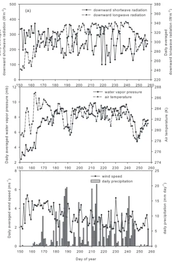
The maximum of 30-min averaged downward shortwave radiation was 1235 Wm−2, 10

and 30-min averaged downward longwave radiation varied from 188 to 388 Wm−2 ing the simulation period. Average downward shortwave and longwave radiations dur-ing total simulation period were 250 Wm−2 and 310 Wm−2, respectively. During the simulation period, the total precipitation at the site was 388 mm over the study period (Fig. 1).

15

Eddy-covariance system consisted of a three dimensional sonic anemometer (CSAT3, Campbell Scientific Inc., Logan, Utah, USA), krypton hygrometer (KH20, Campbell Scientific Inc., Logan, Utah, USA) and a fine-wire thermocouple and their measurement height was 2.9 m above the ground surface (Table 1). The sampling rate was 20 Hz and the data were processed every 30 min for calculating turbulence 20

statistics. Other supporting measurements included radiative fluxes, soil heat fluxes, soil temperature, soil water content, and the profiles of other meteorological variables (i.e., wind speed, humidity, and temperature) (Fig. 1). Detailed descriptions for the site are available in Choi et al. (2004), Yang et al. (2008) and the GAME-Tibet website (http://monsoon.t.u-tokyo.ac.jp/tibet/).

(5)

BGD

6, 10849–10881, 2009

J. Hong and J. Kim

Title Page

Tables Figures

◭ ◮

Back Close

Full Screen / Esc

3 Model simulations

3.1 Model description

To simulate water and energy cycles on the Plateau, we have used two land surface models (LSMs): Simple Biosphere Model 2 (SiB2) and Noah LSM (version 2.7) (Ta-ble 2). The SiB2 incorporates a photosynthesis-conductance model and calculates soil 5

temperature through the force-restore method (two layer model). The soil moisture is computed using the diffusion equation at the soil surface layer, root zone, and deep soil layer, respectively. For calculating radiative transfer within the canopy, SiB2 uses the two-stream approximation, and albedo of soil surface and vegetation depends on soil and vegetation properties as well as on wavelength of incident radiation.

10

The Noah LSM adopts the Zilitinkevich parameter to consider the difference of rough-ness length between momentum and heat (Zilitinkevich, 1995). It calculates both soil temperature and soil moisture content at the same depth, and the number of soil layers is changeable from 2 to 20. Albedo is prescribed by users on a monthly basis before running Noah LSM and this prescribed monthly albedo is linearly interpolated into daily 15

values.

For the calculation of turbulence fluxes, both models use the Monin-Obukhov (MO) similarity. The main contrast between the two models is a way to calculate canopy con-ductance. Noah LSM adopts the empirical functions to limit maximum canopy conduc-tance (gc) proposed by Jarvis (1976). In SiB2, canopy conductance is computed from

20

canopy photosynthesis-conductance model (Sellers et al., 1996b). SiB2 also requires aerodynamic parameters such as the zero-plane displacement height and roughness length for describing turbulent exchanges above and within canopy. These aerody-namic parameters were estimated using MOMPT program in this study (Sellers et al., 1996b). The numerical integration was done every 30 min using the observed driving 25

meteorological variables and initial conditions for soil temperature and soil moisture were defined based on the field observations (Table 1).

(6)

BGD

6, 10849–10881, 2009

J. Hong and J. Kim

Title Page

Tables Figures

◭ ◮

Back Close

Full Screen / Esc

3.2 Input parameters and initial conditions

Initial values and phenological parameters for running the two models were taken from the data observed at the site. In this study, the types of vegetation and soil at the site were assigned to “Agricultural/C3 grassland” and “sandy loam” in the mod-els and default vegetation/soil-type dependent parameters were adopted. No pa-5

rameter calibration was allowed so that we scrutinized structural deficiencies of the models. Detailed values of soil/vegetation-type dependent parameters are available at Zobler (1986) and Sellers et al. (1996a) for SiB2 and “http://www.emc.ncep.noaa. gov/mmb/gcp/noahlsm/Noah LSM USERGUIDE 2.7.1.doc”, Cosby et al. (1984) and van der Velde et al. (2009) for Noah model. Based on the field observations, canopy 10

top and bottom heights for SiB2 were set to 0.05 m and 0.005 m, respectively. Con-currently, rooting depth was set to 0.3 m and the depth of each soil layer in SiB2 (soil surface layer, root zone, and deep soil layer) was 0.07, 0.23, and 1.2 m, respectively. The depth of the first soil layer in SiB2 was obtained from the observed soil temper-ature profiles for the force-restore method (Arya, 2001). In Noah LSM the number of 15

soil layers was set to four, and the depth of soil layer was 0.07, 0.23, 0.5, and 0.7 m, respectively. The observed monthly averaged surface albedo was pre-defined to match the simulated reflected shortwave radiation to the observed values for Noah LSM. How-ever, for SiB2, the default albedo was used with vegetation and soil type as well as the different wavelength.

20

4 Results and discussion

4.1 Roughness length

(7)

BGD

6, 10849–10881, 2009

J. Hong and J. Kim

Title Page

Tables Figures

◭ ◮

Back Close

Full Screen / Esc

Interactive Discussion be fixed throughout the simulation period and was assigned to mean roughness length

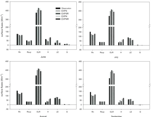
in this study. To examine the sensitivity of the simulated SEB to roughness length, the models were driven by two different roughness lengths (0.001 and 0.01 m) (Fig. 2).

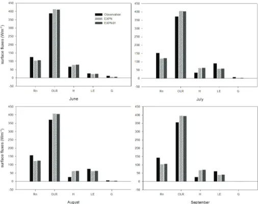
With an increase of the roughness length, both sensible (H) and latent heat fluxes (LE) slightly increased, whereas surface temperature decreased in Noah LSM (i.e., 5

reduction of OLR). Consequently, outgoing longwave radiation (OLR) reduced and hence net radiationRnincreased in Noah LSM. Our interpretation is that the increase

of roughness length enhanced turbulent fluxes and such enhanced turbulent fluxes reduced surface temperature. By contrast, SiB2 showed different responses to the increase of roughness length probably due to the lack of coherence among the aero-10

dynamic parameters in the subroutine EXPSR. In the EXPSR of SiB2 simulation, a con-stant roughness length was decided by force irrespective of the variation of vegetation cover fraction and LAI. In general, our interpretations below do not depend on such variation of roughness lengths and therefore we discussed the results from EXPS and EXPN with the observation data in the following sections.

15

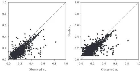
4.2 Friction velocity

Figure 3 demonstrates the simulated friction velocity (u∗) against the observed values. In general, the two models reproduced the observed friction velocity reasonably well. Nevetherless, two features are worth noting: (1) Noah LSM simulated largeru∗ than SiB2 particularly whenu∗ was small, thus reproducing more comparableu∗to the ob-20

servation; and (2) Noah LSM was not successful to replicateu∗<0.07ms −1

.

We noted that theu∗values simulated by SiB2 were smaller than those by Noah LSM particularly during the pre-monsoon season and then tended to become comparable as the monsoon progressed (not shown here). Our analysis showed that such a diff er-ence was related to the parameterization of convection velocity (w∗) which is used in 25

calculatingu∗. Typically,u∗is computed as:

u2

∗=CMu 2

(8)

BGD

6, 10849–10881, 2009

J. Hong and J. Kim

Title Page Abstract Introduction Conclusions References Tables Figures ◭ ◮ ◭ ◮ Back Close

Full Screen / Esc

Interactive Discussion where CM is the drag coefficient. Equation (1) is adopted in SiB2 with a minimum

wind speed of 0.25 ms−1. In Noah LSM, however, w∗ is added in computing u∗ with a minimum wind speed of 0.01 ms−1and a minimum friction velocity of 0.07 ms−1:

u2

∗=CM

u

q

u2+w∗2

(2) wherew∗ is given as

5

w∗=β

2

g

270·1000·CHu

θa−θs

∝H (3)

whereβis an empirical parameter (=1.2) andCHis the turbulent exchange coefficient

for heat. The convection velocity w∗ was proposed for stable numerical integration because mesoscale horizontal wind causes a finite effective friction velocity even in the limit of zero mean wind when local free convection prevails in the surface layer 10

(Businger, 1973; H ¨ogstrom, 1996). To remedy these conditions in the model, there is the prescribed minimum wind speed (u≥0.25ms−1) in SiB2. However, Noah LSM assigns the minimum friction velocity (u∗≥0.07ms

−1

) and also convection velocity for the numerically stable simulation in calm conditions, which explains the minimum u∗ manifested in Fig. 3.

15

In the nighttime conditions, the convection velocity turns off. In the daytime, however, the magnitude ofw∗was sometimes compatible to the mean wind speed on the Plateau when the wind was calm and vertical gradient of temperature was large, i.e., a typical condition in the pre-monsoon season on the Plateau (Fig. 4). Indeed, the convection velocity is proportional toH, and thereforeu∗differences between the two models were 20

larger during the pre-monsoon period whenH was dominant surface fluxes. Without the convection velocity parameterization, the drag coefficient for momentum in Noah LSM became similar to that in SiB2 (not shown).

In Eq. (3), we also note that by default, surface temperature was set to 270 K, and the atmospheric boundary layer (ABL) height 1000 m in Noah LSM. Therefore, the convec-25

(9)

BGD

6, 10849–10881, 2009

J. Hong and J. Kim

Title Page

Tables Figures

◭ ◮

Back Close

Full Screen / Esc

Interactive Discussion on the Plateau were higher than those fixed values, especially during the daytime in the

summer season. Over the ocean surface where the diurnal variation of surface temper-ature is weak, the constant ABL height of 1000 m may not induce substantial bias (e.g., Zeng et al., 1998). Also, such an overestimation ofw∗helps numerical integration to be stable in the atmosphere-vegetation coupled model without the bias of model results 5

due to negative feedback (McNaughton and Jarvis, 1991; Kaimal and Finnigan, 1994). There is, however, no regulation process in the off-line simulation and the bias of inw∗ clearly makes an impact when the biosphere models were driven using the observed data particularly on the Tibetan Plateau during the pre-monsoon season.

The w∗ parameterization was derived for the case when the time average of wind 10

speed (u) was replaced by the speed of the time-averaged wind vector (pu2₊_v2₎

for the stable time integration of numerical models (Beljaars, 1995; Mahrt and Sun, 1995). In the present study, the time averaged wind vector from a 3-dimensional sonic anemometer was used for driving the two models. When a biosphere model is driven by the time average of wind speed from a cup anemometer, however, it may be inap-15

propriate to includew∗in the aerodynamic bulk formula. Such differences of mean wind speed have not been clearly pointed out in most model studies but become important when the wind meandering is substantial.

4.3 Sensible heat fluxes

The two models overestimated H against the observation. In particular, H in Noah 20

LSM was larger than in SiB2 (Fig. 2). Plausible explanations about the differences inH

between the models are 1) the difference in simulated Ts which is expressed by OLR

and 2) the di_fference in aerodynamic conductance.

The sensible heat flux is proportional to surface temperature in the models and thus larger Ts in Noah LSM had a direct influence on H. Our analysis revealed that this

25

largerTsin Noah LSM mainly resulted from the underestimation of soil evaporation. As

will be shown later, the Noah LSM underestimated soil evaporation and theTs diff

(10)

BGD

6, 10849–10881, 2009

J. Hong and J. Kim

Title Page

Tables Figures

◭ ◮

Back Close

Full Screen / Esc

Interactive Discussion ence largely disappeared when the soil evaporation in the models was adjusted. Also,

using the same models, Hong and Kim (2008) showed that inaccurate assignments of surface albedo and emissivity can make substantial bias inTs simulation between

the two models on the Plateau. In addition, the overestimatedH during the nighttime in Noah LSM can be attributed to the overestimation of aerodynamic conductance ne-5

cessitating an adjustment of the minimum wind and friction velocities before testing the model.

The inhomogeneity of transfer mechanisms between momentum and heat is another factor contributing to the difference between the drag coefficients for heat (CH) and

mo-mentum (CM). This difference results from the surface heterogeneity as well as the

10

pressure terms in the momentum conservation equation, which are handled differently in the two models. The different transfer mechanism between momentum and heat has been one of the critical issues in boundary layer meteorology (e.g., Garratt, 1992; Brutsaert and Mawdsley, 1996; Chen et al., 1997; Lhomme et al., 2000; Sch ¨uttemeyer et al., 2008; Yang et al., 2008) and the difference is commonly expressed by the Zil-15

itinkevich parameter,C(Zilitinkevich, 1995) or Stanton number,B:

kB−1

=ln _z

m0

zh0

=kCpRe (4)

Equation (4) suggests that the reduction ofCincreasesCHby increasingzh0. Surface

temperature becomes lower, butRnandH increase with the reduction ofC.

The parameterCis related to soil status, land cover type, and vegetation coverage. 20

Its value is within the range from 0.1 to 0.4 (Chen et al., 1997) and closely related to the model performance. For example, Beljaars and Viterbo (1994) found that an over-estimation of evaporation in the winter is reduced whenzm0/zh0=10. Hopwood (1995)

concluded thatz_m0/z_h0would be∼80 for an inhomogeneous land surface. Chen et al.

(1997) also pointed out that the effect of large C becomes more apparent when the 25

soil gets drier and the skin temperature higher (i.e., similar to the environment of the Plateau). Furthermore,zm0/zh0 is likely to become very small for sparse canopy

(11)

BGD

6, 10849–10881, 2009

J. Hong and J. Kim

Title Page

Tables Figures

◭ ◮

Back Close

Full Screen / Esc

Interactive Discussion reported that, the ratio ofzm0/zh0 shows diurnal variation with atmospheric conditions

(e.g., Su et al., 2001; Yang et al., 2003, 2008).

In Noah LSM, C was prescribed as 0.4. The parameterization of C is, however, not considered explicitly in SiB2 because aerodynamic resistance for heat is cal-culated from aerodynamic conductance for momentum, causing the differences in 5

gh(≡_ρCH p(

1

θ−θs

)) between the two models. Figure 5 shows the sensitivity of the sim-ulated surface fluxes onC in Noah LSM. WhenC diminished from 0.4 to 0.1, Rn, H,

and LE increased, but Ts decreased. The gh of Noah LSM was larger than that of

SiB2 for a given roughness length and the difference inghdiminished with increasing

C. In contrast, the reduction ofgh increases the bias ofRn between the models. The

10

simulation of surface temperature, sensible heat flux, and soil heat flux on the Plateau has improved by considering the diurnal variation ofCin the model (e.g., Yang et al., 2009). In our study, however, the alteration of C did not produce concurrent reduc-tions in inter-model biases of all the surface flux components includingRn andLE on

a monthly scale. 15

The two biosphere models assume that the source/sink distributions between tem-perature and water vapor are the same and the turbulent transfer satisfies the MO similarity (i.e., uniform distribution of scalars and no impact of entrainment process). On the Plateau, however, the source/sink distribution of water vapor is not the same as that of heat due to seasonal variations associated with the Asian monsoon (Choi 20

et al., 2004). Moreover, scalar fluxes can be enhanced from the prediction of the MO similarity because of the role of outer turbulence, that do not contribute to momentum fluxes but scalar fluxes in the surface layer (McNaughton and Brunet, 2002; Hong et al., 2004; McNaughton et al., 2007). Hence, the models, which are based on the MO sim-ilarity, can underestimate scalar fluxes. Recently, McNaughton et al. (2007) proposed 25

the outer dissipation rate to remedy the MO similarity and further study should be done to resolve this issue in the future.

(12)

BGD

6, 10849–10881, 2009

J. Hong and J. Kim

Title Page

Tables Figures

◭ ◮

Back Close

Full Screen / Esc

4.4 Latent heat fluxes

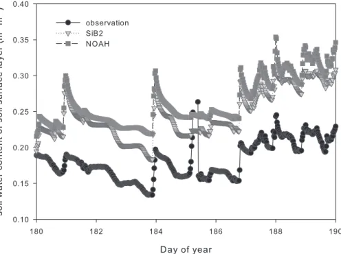
The two models overestimated soil water contentθbut reproduced the observed diur-nal and seasodiur-nal patterns fairly well (Fig. 6). With the bias inθ, the two models showed di_fferent partitioning of rainfall into evapotranspiration (Fig. 7). To quantify the e_ffect of soil moisture bias in the models and the observation, we conducted control simula-5

tions by forcing the observedθ into the models at each time step (i.e., reducing θ in the models). In this control simulation,Rnand LE decreased but H increased as

ex-pected. Desipite the similarθ and smaller aerodynamic conductance, SiB2 produced consistently largerLE, for which different explanation was necessary.

LE was divided into soil evaporation (LEg) and transpiration (LEc). Figures 7 and 8

10

show that the two models showed similarLEcand the difference was mainly originated

from LEg. It is also noted that the ratio of LEg to total LE was biased against the

observation data (Fig. 8). We found that the difference in LEgresulted from the use of

a different formula for computingLEg. Soil evaporation in Noah LSM is formulated as:

LEg=λ

_φ₋_φ

th

φ_s−φ_th

F

(1−W_g)·E_p (5)

15

The bare soil evaporation exponent, F is one of the site-dependent parameters and was set to a default value of 2.0 in this study. In SiB2, different formula is used:

LEg=λ

₍_h

soiles(Ts)−ea)

rsoil+rd

ρc

p

γ (1−Wg) (6)

Sellers et al. (1992) included rsoil to prevent the excessive soil evaporation rate and

this resistance was estimated from the time series of station data from the FIFE (First 20

ISLSCP Field Experiment) project using a series of inverse-mode runs with SiB2:

rsoil=e8.206

−4.255W1 ₍₇₎

Againrsoil is a site-specific parameter. In particular, Rn and G were forced to match

(13)

BGD

6, 10849–10881, 2009

J. Hong and J. Kim

Title Page

Tables Figures

◭ ◮

Back Close

Full Screen / Esc

Interactive Discussion Theδ18O isotope measurement at the same site suggested that approximately 27%

of the precipitation be lost by evaporation from soil surface during monsoon (Tsujimura et al., 2001). For estimating the impact of soil evaporation submodels in the models, the two models have been re-simulated after adapting soil evaporation in such a way that the simulatedLEg was same with the observed LEg. Such an adjustment produced

5

an increasedθ in SiB2 but a decrease in Noah LSM. This simulation result leads us to conclude that soil evaporation is a main factor for consistent simulation of SEB over the Plateau (Fig. 9). It is important to note that we adapted the soil evaporation using the soil water contents overestimated by the two models, suggesting the need for the improvement of soil hydrology in the biosphere models. Despite such adaptation, the 10

simulated soil water contents were still larger than the observed, and therefore other components of water budget (e.g., runo_ff) should be carefully assessed.

4.5 Soil heat fluxes

The soil heat flux (G), exceeding>200Wm−2 during the daytime in the pre-monsoon season, plays a substantial role in surface energy partitioning on the Plateau (e.g., Choi 15

et al., 2004; Gao, 2005). In general, both models reproduced the observed diurnal variations as well as monthly means of G (Figs. 2 and 10). The monthly averaged energy residual in Noah LSM was about−2∼−4 Wm−2, and the sum of residual and

G in Noah LSM was nearly the same asG in SiB2. We note, however, that the two models simulated soil temperature and soil water contents differently and G in SiB2 20

was more sensitive to the radiative forcing than Noah LSM. Part of the reason may be explained by smaller soil heat capacity in SiB2.

Different formulations for soil heat capacity are used in the two models. In SiB2, soil heat capacity is calculated following Camilo and Schmugge (1981):

Csoil=

0.5(1−φ_s)+φ·W₁·(4.816×106) (8)

25

In Noah LSM, soil heat capacity is calculated as:

Csoil=φ·Cw+(1−φs)·Cs+(φs−φ)·Cair (9)

(14)

BGD

6, 10849–10881, 2009

J. Hong and J. Kim

Title Page

Tables Figures

◭ ◮

Back Close

Full Screen / Esc

Interactive Discussion Note that the observedG is based on Eq. (9). TheCsoil in SiB2 is larger (within 5%)

than that in Noah LSM for a given soil moisture content. The two models, however, simulatedθdifferently. Consequently, soil heat capacity in SiB2 was 20% smaller than that in Noah LSM, thereby increasing temporal variations ofGin SiB2.

The SiB2 calculatesGusing the force-restore method whereas the Noah LSM calcu-5

latesGusing the diffusion equation independently of other energy budget components. If we neglect the energy transfer due to phase changes in water and snow, the Force-Restore method is formulated as:

G=Cg

∂Tg

∂t +

2πCd

τd

(Tg−Td)=Rn−H−LE (10)

In this formulation, soil is divided into two layers andG is calculated at each time step 10

after computingRn,H andLE.

Theoretically, the depth of soil surface layer in the force-restore method is half of the damping depth for the diurnal soil thermal wave (Garratt, 1992; Arya, 2001). The damping depth depends not only on soil physical properties, but also on the soil mois-ture content. In reality, the damping depth varied from 0.05 to 0.14 m on the Plateau as 15

the monsoon progressed (not shown). The depth of the first soil layer in SiB2 was, how-ever, constant during the simulation period. Indeed, an increase of the depth of the soil surface layer results in an increase of the Bowen ratio. Based on the observed damp-ing depth on the Plateau, the depth of the soil surface layer in SiB2 tended to partition more energy intoLE during the monsoon period. Consequently, one should consider 20

the variations in the depth of soil surface layer with time for long-term simulation.

5 Summary and conclusions

(15)

BGD

6, 10849–10881, 2009

J. Hong and J. Kim

Title Page

Tables Figures

◭ ◮

Back Close

Full Screen / Esc

Interactive Discussion data, the two biosphere models did not provide convergent estimates of surface fluxes

throughout the simulation period including the seasonal march of the summer mon-soon. The biases between the models were related mainly to 1) different aerodynamic conductance due to the convection velocity parameterization; 2) inhomogeneity of tur-bulent transfer between momentum and scalars; and 3) di_fferent formulations of direct 5

soil evaporation. The structural deficiencies of the model seen in this study can be manifested in simulating SEB in other altitudes and latitudes as well.

The 18O stable isotope data provided critical information on validating and analyz-ing the simulated evapotranspiration by the biosphere models. Our findanalyz-ings reaffirm the importance of careful interpretations of the modeling outputs due to uncertainties 10

inherent in the models and the significance of in-situ field observations in modeling SEB on the Tibetan Plateau. For an accurate modeling of SEB on the Plateau, more attention should be given to retrieving information about the soil properties, which also emphasizes the di_fficulty in interpreting the modeling outputs on the Plateau without constraints that are based on field observations.

15

Appendix A

Notations

cp specific heat of air

ea atmospheric vapor pressure

20

es saturated atmospheric vapor pressure

g gravity constant

gc canopy conductance

gh aerodynamic conductance for heat

hsoil relative humidity at soil surface

25

(16)

BGD

6, 10849–10881, 2009

J. Hong and J. Kim

Title Page

Tables Figures

◭ ◮

Back Close

Full Screen / Esc

rd aerodynamic resistance between ground and canopy

air surface

rsoil bare soil surface resistance

t time (second)

u streamwise wind speed 5

u∗ friction velocity

zm0 roughness length for momentum

zh0 roughness length for heat

w∗ convective velocity scale

B Stanton number 10

C Zilitinkevich parameter

Cair heat capacity of air

Cd heat capacity of deep soil layer in SiB2

Cg heat capacity of surface soil layer in SiB2

CH turbulent exchange coefficient for heat

15

CM drag coefficient for momentum

Cs heat capacity of mineral soil

Csoil heat capacity of soil

Cw heat capacity of water

Ep potential evaporation

20

G soil heat flux

H sensible heat flux

LE latent heat flux

(17)

BGD

6, 10849–10881, 2009

J. Hong and J. Kim

Title Page

Tables Figures

◭ ◮

Back Close

Full Screen / Esc

LEg latent heat flux from soil

Re Reynolds number

Rn net radiation

Td deep soil temperature in SiB2

Tg surface soil temperature in SiB2

5

T_s surface temperature

Wg vegetation cover fraction

W1 soil wetness fraction≡θ/θs

θ mean potential temperature of air

θs mean potential temperature of ground surface

10

φ soil water content

φs porosity

φth soil water content threshold in Noah LSM

ρ air density

τd day length≡86400s

15

Acknowledgements. We acknowledge H. P. Schmid, S. Y. Hong and anonymous reviewers for their valuable comments on this manuscript. This research was supported by Advanced Research on Meteorological Sciences (NIMR-2009-C-1) of the National Institute of Meteoro-logical Research/Korea MeteoroMeteoro-logical Administration, the BK21 program from the Ministry of Education and Human Resources Management of Korea, a grant (code: 1-8-3) from

Sustain-20

able Water Resources Research Center for 21st Century Frontier Research Program and the “CarboEastAsia” A3 Foresight program of the Korean Science and Engineering Foundation.

(18)

BGD

6, 10849–10881, 2009

J. Hong and J. Kim

Title Page

Tables Figures

◭ ◮

Back Close

Full Screen / Esc

References

Arya, S. P.: Introduction to Micrometeorology, Academic Press, San Diego, California, 2001. 10854, 10862

Beljaars, A. C.: The parameterization of surface fluxes in large-scale models under free con-vection, Q. J. Roy. Meteor. Soc., 121, 255–270, 1995. 10857

5

Beljaars, A. C. and Viterbo, P.: The sensitivity of winter evaporation to the formulation of aero-dynamic resistance in the ECMWF model, Bound.-Lay. Meteorol., 71, 135–149, 1994. 10858 Brutsaert, W. and Mawdsley, J. A.: Sensible heat transfer parameterization for surfaces with

anisothermal dense vegetation, J. Atmos. Sci., 53, 209–216, 1996. 10858

Businger, J. A.: A note on free convection, Bound.-Lay. Meteorol., 4, 323–326, 1973. 10856

10

Camilo, P. and Schmugge, T. J.: A computer program for the simulation of heat and moisture flow in soils, in: NASA Tech. Memo. 82121, Maryland, USA, 1981. 10861

Chen, F., Janjic, Z., and Mitchell, K.: Impact of atmospheric surface-layer parameterizations in the new land-surface scheme of the NCEP mesoscale ETA model, Bound.-Lay. Meteorol., 85, 391–421, 1997. 10858

15

Chen, L., Reiter, E. R., and Feng, Z.: The atmosphere heat source over the Tibetan Plateau: May–August 1979, Mon. Weather Rev., 113, 1771–1790, 1985. 10851

Choi, T., Hong, J., Kim, J., Lee, H. C., Asanuma, J., Ishikawa, H., Tsukamoto, O., Zhiqiu, G., Ma, Y., Ueno, K., Wang, J., Koike, T., and Yasunari, T.: Turbulent exchange of heat, water vapor and momentum over a Tibetan Prairie by Eddy covariance and flux-variance

measure-20

ments, J. Geophys. Res., 109, D21106, doi:10.1029/2004JD004767, 2004. 10852, 10859, 10861

Cosby, B. J., Hornberger, G. M., Clapp, R. B., and Ginn, T. R.: A statistical exploration of the relationships of soil moisture characteristics to the physical properties of soils, Water Resour. Res., 20, 682–690, 1984. 10854, 10871

25

Denman, K. L., Brasseur, G., Chidthaisong, A., Ciais, P., Cox, P., Dickinson, R., Hauglus-taine, D., Heinze, C., Holland, E., Jacob, D., Lohmann, U., Ramachandran, S., da Silva Dias, P., Wofsy, S., and Zhang, X.: Couplings between changes in the climate system and biogeochemistry, in: Climate Change 2007: The Physical Science Basis. Contri-bution of Working Group I to the Fourth Assessment Report of the Intergovernmental Panel

30

(19)

BGD

6, 10849–10881, 2009

J. Hong and J. Kim

Title Page

Tables Figures

◭ ◮

Back Close

Full Screen / Esc

Gao, Z.: Determination of soil heat flux in a Tibetan short-grass prairie, Bound.-Lay. Meteorol., 114, 165–178, 2005. 10861

Gao, Z., Chae, N., Kim, J., Hong, J., Choi, T., and Lee, H.: Modeling of surface energy partition-ing, surface temperature and soil wetness in the Tibetan prairie using the Simple Biosphere Model 2 (SiB2), J. Geophys. Res., 109, D06102, doi:10.1029/2003JD004089, 2004. 10851

5

Garratt, J. R.: The Atmospheric Boundary Layer, Cambridge University Press, 1992. 10858, 10862

H ¨ogstrom, U.: Review of some basic characteristics of the atmospheric surface layer, Bound.-Lay. Meteorol., 78, 215–246, 1996. 10856

Hong, J. and Kim, J.: Simulation of surface radiation balance on the Tibetan Plateau, Geophys.

10

Res. Lett., 35, L08814, doi:10.1029/2008GL033613, 2008. 10851, 10858

Hong, J., Choi, T., Ishikawa, H., and Kim, J.: Turbulence structures in the near-neutral surface layer on the Tibetan Plateau, Geophys. Res. Lett., 31, L15016, doi:10.1029/2004GL 019935, 2004. 10859

Hopwood, W. P.: Surface transfer of heat and momentum over an inhomogeneous vegetated

15

land, Q. J. Roy. Meteor. Soc., 121, 1549–1574, 1995. 10858

Jarvis, P.: The interpretation of the variations in leafwater potential and stomatal conductances found in canopies in the field, Philos. T. R. Soc. Lond., 273, 593–610, 1976. 10853, 10871 Kaimal, J. C. and Finnigan, J. J.: Atmospheric Boundary Layer Flows, Oxford University Press,

1994. 10857

20

Lhomme, J. P., Chehbouni, A., and Monteny, B.: Sensible heat flux-radiometric surface temper-ature relationship over sparse vegetation: Parameterizing B−1

, Bound.-Lay. Meteorol., 97, 431–457, 2000. 10858

Li, C. and Yanai, M.: The onset and interannual variability of the Asian summer monsoon in relation to land-sea thermal constrast, J. Climate, 9, 358–375, 1996. 10851

25

Mahrt, L. and Sun, J.: The subgrid scale in the bulk aerodynamic relationship for spatially averaged scalar fluxes, Mon. Weather Rev., 123, 3032–3041, 1995. 10857

McNaughton, K. G. and Brunet, Y.: Townsend’s hypothesis, coherent structures and Monin-Obukhov similarity, Bound.-Lay. Meteorol., 102, 161–175, 2002. 10859

McNaughton, K. G. and Jarvis, P. G.: Effects of spatial scale on stomatal control of transpiration,

30

Agr. Forest Meteorol., 54, 279–301, 1991. 10857

McNaughton, K. G., Clement, R. J., and Moncrieff, J. B.: Scaling properties of velocity and temperature spectra above the surface friction layer in a convective atmospheric boundary

(20)

BGD

6, 10849–10881, 2009

J. Hong and J. Kim

Title Page

Tables Figures

◭ ◮

Back Close

Full Screen / Esc

layer, Nonlinear Proc. Geoph., 14, 257–271, 2007. 10859

Peylin, P., Polcher, J., Bonan, G., Williamson, D. L., and Laval, K.: Comparison of two complex land surface schemes coupled to the National Center for Atmospheric Research general circulation model, J. Geophys. Res., 102, 19413–19431, 1997. 10851

Sch ¨uttemeyer, D., Holtslag, A. A. M., and de Bruin, H. A. R.: Evaluation of two land surface

5

schemes used in terrains of increasing aridity in west Africa, J. Hydrometerol., 9, 173–193, 2008. 10858

Sellers, P. J., Heiser, M. D., and Hall, F. G.: Relations between surface conductance and spec-tral vegetation indices at intermediate (100 m2to 15 km2) length scales, J. Geophys. Res., 17, 19033–19059, 1992. 10860

10

Sellers, P. J., Los, S. O., Tucker, C. J., Justice, C. O., Dazlich, D. A., Collatz, G. J., and Ran-dall, D. A.: A revised land surface parameterization (SiB2) for atmospheric GCMs. Part II: The generation of global field of terrestrial biophysical parameters from satellite data, J. Climate, 9, 706–737, 1996a. 10854

Sellers, P. J., Randall, D. A., Collatz, G. J., Berry, J. A., Field, C. B., Dazlich, D. A., Zhang, C.,

15

Collelo, G. D., and Bounoua, L.: A revised land surface parameterization (SiB2) for atmo-spheric GCMs. Part I: Model formulation, J. Climate, 9, 676–705, 1996b. 10853, 10871 Su, Z., Schmugge, T., Kustas, W. P., and Massman, W. J.: An evaluation of two models for

estimation of the roughness height for heat transfer between the land surface and the atmo-sphere, J. Appl. Meteorol., 40, 1933–1951, 2001. 10859

20

Takayabu, I., Takata, K., Yamazaki, T., Ueno, K., Yabuki, H., and Haginoya, S.: Comparison of the four land surface models driven by a common forcing data prepared from GAME/Tibet POP97 products-Snow accumulation and soil freezing processes, J. Meteorol. Soc. Japan, 79, 535–554, 2001. 10851

Tsujimura, M., Kim, J., and Asanuma, J.: Surface energy balance, water balance, and stable

25

isotope measurements in the Tibetan plateau, in: Proc. IAMAS, Innsbruck, Austria, 2001. 10861

van der Velde, R., Su, Z., Ek, M., Rodell, M., and Ma, Y.: Influence of thermodynamic soil and vegetation parameterizations on the simulation of soil temperature states and surface fluxes by the Noah LSM over a Tibetan plateau site, Hydrol. Earth Syst. Sci., 13, 759–777, 2009,

30

http://www.hydrol-earth-syst-sci.net/13/759/2009/. 10851, 10854

(21)

BGD

6, 10849–10881, 2009

J. Hong and J. Kim

Title Page

Tables Figures

◭ ◮

Back Close

Full Screen / Esc

Yang, K., Koike, T., Ishikawa, H., Kim, J., Li, X., Liu, H., Liu, S. M., Ma, Y., and Wang, J. M.: Turbulent flux transfer over bare-soil surfaces: Characteristics and parameterization, J. Appl. Meteorol., 47, 276–290, 2008. 10851, 10852, 10858, 10859

Yang, K., Chen, Y.-Y., and Qin, J.: Some practical notes on the land surface modeling in the Tibetan Plateau, Hydrol. Earth Syst. Sci., 13, 687–701, 2009,

5

http://www.hydrol-earth-syst-sci.net/13/687/2009/. 10851, 10859

Zeng, X., Zhao, M., and Dickinson, R. E.: Intercomparison of bulk aerodynamic for the compu-tation of sea surface fluxes using TOGA COARSE and TAO data, J. Climate, 11, 2628–2644, 1998. 10857

Zilitinkevich, S. S.: Non-local turbulent transport: Pollution dispersion aspects of coherent

struc-10

ture of convective flows, in: Air Pollution-Volume III, Air Pollution Theory and Simulation, edited by: Power, H., Moussiopoulos, N., and Brebbia, C. A., 53–60, Computational Me-chanics Publications, Southampton, Boston, 1995. 10853, 10858, 10871

Zobler, L.: A world soil file for global climate modeling, in: NASA Tech. Memo. 87802, Maryland, USA, 1986. 10854, 10871

15

(22)

BGD

6, 10849–10881, 2009

J. Hong and J. Kim

Title Page

Tables Figures

◭ ◮

Back Close

Full Screen / Esc

Table 1.The observed meteorological variables.

Variable Instrumentation Height

(23)

BGD

6, 10849–10881, 2009

J. Hong and J. Kim

Title Page

Tables Figures

◭ ◮

Back Close

Full Screen / Esc

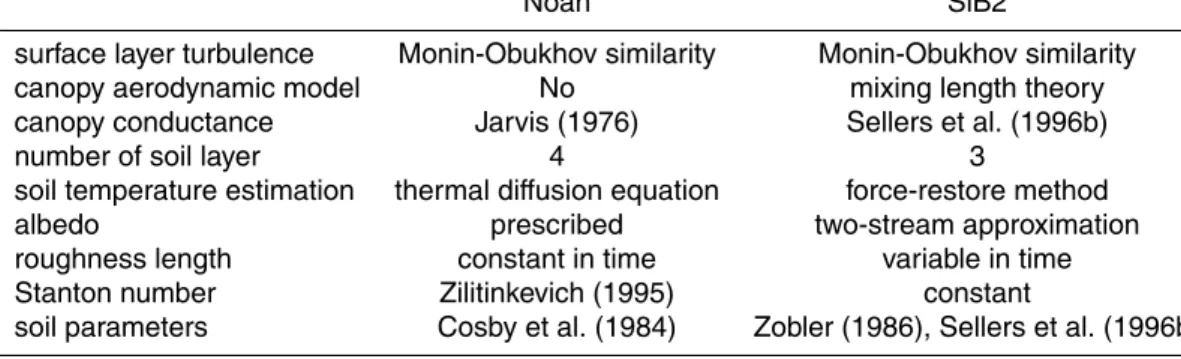
Table 2.Summary of the model structure and soil/canopy parameters of Noah and SiB2.

Noah SiB2

surface layer turbulence Monin-Obukhov similarity Monin-Obukhov similarity canopy aerodynamic model No mixing length theory canopy conductance Jarvis (1976) Sellers et al. (1996b)

number of soil layer 4 3

soil temperature estimation thermal diffusion equation force-restore method

albedo prescribed two-stream approximation

roughness length constant in time variable in time Stanton number Zilitinkevich (1995) constant

soil parameters Cosby et al. (1984) Zobler (1986), Sellers et al. (1996b)

(24)

BGD

6, 10849–10881, 2009

J. Hong and J. Kim

Title Page

Tables Figures

◭ ◮

Back Close

Full Screen / Esc

(25)

BGD

6, 10849–10881, 2009

J. Hong and J. Kim

Title Page

Tables Figures

◭ ◮

Back Close

Full Screen / Esc

Fig. 2. Monthly averaged surface flux at the site. EXPS and EXPN denote the simulation of SiB2 and Noah LSM with 0.001 m of roughness length, which is calculated from MOMOPT program. EXPSR and EXPNR denote the simulation of SiB2 and Noah LSM with 0.01 m of roughness length.

(26)

BGD

6, 10849–10881, 2009

J. Hong and J. Kim

Title Page

Tables Figures

◭ ◮

Back Close

Full Screen / Esc

(27)

BGD

6, 10849–10881, 2009

J. Hong and J. Kim

Title Page

Tables Figures

◭ ◮

Back Close

Full Screen / Esc

Fig. 4. 30-min averaged mean wind speed and convection velocity calculated in Noah LSM before and during monsoon period.

(28)

BGD

6, 10849–10881, 2009

J. Hong and J. Kim

Title Page

Tables Figures

◭ ◮

Back Close

Full Screen / Esc

(29)

BGD

6, 10849–10881, 2009

J. Hong and J. Kim

Title Page

Tables Figures

◭ ◮

Back Close

Full Screen / Esc

Fig. 6. Comparison of simulated soil moisture contents (0–7 cm) with the observed soil mois-ture contents (0–0.1 m)

(30)

BGD

6, 10849–10881, 2009

J. Hong and J. Kim

Title Page

Tables Figures

◭ ◮

Back Close

Full Screen / Esc

(31)

BGD

6, 10849–10881, 2009

J. Hong and J. Kim

Title Page

Tables Figures

◭ ◮

Back Close

Full Screen / Esc

Fig. 8.Partitioning of evapotranspiration into soil evaporation and transpiration in the models.

(32)

BGD

6, 10849–10881, 2009

J. Hong and J. Kim

Title Page

Tables Figures

◭ ◮

Back Close

Full Screen / Esc

Fig. 9. The simulated surface energy partitioning: the simulation results before(A)and after

(33)

BGD

6, 10849–10881, 2009

J. Hong and J. Kim

Title Page

Tables Figures

◭ ◮

Back Close

Full Screen / Esc

Fig. 10.Diurnal variation of soil heat fluxes.