www.earth-syst-dynam.net/2/161/2011/ doi:10.5194/esd-2-161-2011
© Author(s) 2011. CC Attribution 3.0 License.
Earth System
Dynamics
A multi-model ensemble method that combines imperfect models
through learning
L. A. van den Berge1, F. M. Selten1, W. Wiegerinck2, and G. S. Duane3
1Royal Netherlands Meteorological Institute, Wilhelminalaan 10, 3732 GK De Bilt, The Netherlands 2Donders Institute for Brain, Cognition and Behaviour, Radboud University Nijmegen, Geert Grooteplein 21, 6525 EZ Nijmegen, The Netherlands
3Department of Atmospheric and Oceanic Sciences, University of Colorado, Boulder, CO 80309, USA Received: 6 July 2010 – Published in Earth Syst. Dynam. Discuss.: 1 October 2010
Revised: 15 June 2011 – Accepted: 16 June 2011 – Published: 30 June 2011
Abstract.In the current multi-model ensemble approach cli-mate model simulations are combined a posteriori. In the method of this study the models in the ensemble exchange in-formation during simulations and learn from historical obser-vations to combine their strengths into a best representation of the observed climate. The method is developed and tested in the context of small chaotic dynamical systems, like the Lorenz 63 system. Imperfect models are created by perturb-ing the standard parameter values. Three imperfect models are combined into one super-model, through the introduction of connections between the model equations. The connec-tion coefficients are learned from data from the unperturbed model, that is regarded as the truth.
The main result of this study is that after learning the super-model is a very good approximation to the truth, much better than each imperfect model separately. These illustra-tive examples suggest that the super-modeling approach is a promising strategy to improve weather and climate simula-tions.
1 Introduction
There is a broad scientific consensus that our climate is warming due to anthropogenic emissions of greenhouse gasses (IPCC, 2007). Due to the large impacts of climate change on society there is a growing need to widely sample and assess the possible climate change related to the plausi-ble scenarios for future emissions. At about a dozen climate
Correspondence to:F. M. Selten ([email protected])
institutes around the world complex climate models have been developed over the past decades. Despite the improve-ments in the quality of the model simulations, the models are still far from perfect. For instance a temperature bias of sev-eral degrees in annual mean temperatures in large regions of the globe is not uncommon in the simulations of the present climate (IPCC, 2007).
Nevertheless these models are used to simulate the re-sponse of the climate system to future emission scenarios of greenhouse gasses. It turns out that the models differ substantially in their simulation of the response: the global mean temperature rise varies by as much as a factor of 2 and on regional scales the response can be reversed, e.g. de-creased precipitation instead of an increase. It is not clear how to combine these outcomes to obtain the most realistic response. The standard approach is to take some form of a weighted average of the individual outcomes (Tebaldi and Knutti, 2007), but is this the best strategy?
We think we can do better by letting the models exchange information during the simulation instead of combining the results of the individual models afterwards. We propose to combine the individual models into one super-model by pre-scribing connections between the model equations. The con-nection coefficients are learned from historical observations. This way the super-model learns to combine the strengths of the individual models in order to optimally reproduce the historical climate. Is this approach feasible?
coupling the momentum fluxes from one model and the heat and fresh water fluxes from the other to the ocean model.
Another indication that this approach might be feasible is found in the practice of data assimilation (Compo et al., 2006). It turns out that with a limited amount of informa-tion, the complete state of the atmosphere can be recovered. Synchronization in chaotic systems provides an explanation why this is at all possible, since linking chaotic systems with a signal from one system to the other is known to lead to syn-chronization of their states (Pecora and Carroll, 1990; Duane et al., 2006). Therefore we expect that in the super-modeling approach only limited information needs to be exchanged to effectively influence the combined behaviour of the imper-fect models.
In this paper we use simple chaotic systems to develop and demonstrate the super-modeling approach. We regard the model with standard parameter values as ground truth and create imperfect models by perturbing the parameter values. Three imperfect models are connected and combined into a super-model. The strength of the connections are determined from data from the ground truth through a learning process. The learning process takes the form of the minimisation of a cost function that measures the difference between the truth and the super-model during short integrations.
In Sect. 2 the form of the connections is introduced, fol-lowed by the introduction of the cost function and the min-imisation method. The super-modeling approach is applied to the Lorenz 63, R¨ossler and Lorenz 84 systems in Sects. 3 and 4. Discussion and conclusion of the method and ideas for improvement can be found in Sect. 5.
2 The super-modeling approach
To introduce the super-modeling approach we use the Lorenz 63 system (Lorenz, 1963). The Lorenz 63 system is often used as a metaphore for the atmosphere, because of its abrupt regime changes and unstable nature. The equations for the Lorenz 63 system are
˙
x=σ (y −x) ˙
y=x (ρ −z) −y (1)
˙
z=xy −βz.
The standard parameter values are σ= 10, β=83 and ρ= 28. Numerical solutions are obtained by a fourth order Runge-Kutta time stepping scheme, with a time step of 0.01.
2.1 Connecting imperfect models
Imperfect models are created by taking three copies of the Lorenz 63 system with perturbed parameter values. A super-model is created by the introduction of linear connection terms
˙
xk =σk (yk −xk) + X
j6=k
Ckjx xj − xk
˙
yk =xk (ρk −zk) −yk + X
j6=k
Ckjy yj −yk (2) ˙
zk =xk yk−βkzk + X
j6=k
Ckjz zj−zk, k = 1,2,3,
wherek indexes the three imperfect models with perturbed parameter values σk, βk andρk andCkjx, Ckjy and Ckjz are referred to as connection coefficients.
Each variable of each model is connected to the other two models. This gives two connection coefficients for each of the variables and a total number of 2×3×3 = 18 connec-tion coefficients. These 18 coefficients will be learned from data that sample the truth. The solution of the super-model, denoted by subscript “s”, is taken to be the average of the imperfect models
xs = 1
3 (x1 +x2 +x3) ys =
1
3 (y1 +y2 +y3) (3)
zs = 1
3 (z1+z2 +z3).
Note that Eqs. (2) define a new dynamical system with three times the number of degrees of freedom. The super-model is not merely a sort of average system. Depending on the connections, it can have a very different dynamics. The super-model has the potential to outperform the ensem-ble averaged simulations of the individual models because it can display richer dynamical behavior. The learning must ensure that the behavior after learning is more realistic.
2.2 Cost function
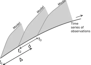
We assume that we have a long time series of observations of the truthxo. We pick initial conditionsxo(ti)from this long time series atKtimesti,i= 1, ...,K, separated by fixed distancesd. Short integrations of length 1are performed with the super-model starting from these K initializations (see Fig. 1). To measure the ability of the super-model to follow the truth we introduce the following cost functionF, that depends on the vector of connection coefficientsC.
F (C)= 1 K1
K X
i=1 Z ti+1
ti
|xs(C, t)−xo(t )|2γt dt (4)
Fig. 1.The cost function is based on short integrations of the super-model starting from observed initial conditions of the truth at times
tiand measures the mean-squared difference between the short
evo-lutions of the super-model and the truth as indicated by the shaded areas. The short integrations span a time interval1andddenotes the fixed time interval between the initial conditionsti.
different initial conditions and leads to a non-zero cost func-tion due to chaos. This implies that the cost funcfunc-tion mea-sures a mixture of model errors and internal error growth. Model errors dominate the inital divergence between model and truth, but at later times in the short term integrations in-ternal error growth dominates. Since we wish to measure the model errors, the factorγt discounts the errors at later times to decrease the contribution of internal error growth.
We base the choice ofγ on the doubling time of errors. From a large number of runs (107) from randomly perturbed initial conditions we estimate the average doubling timeτ of the initial error. We chooseγ such thatγτ=12, so at time τ the weight is reduced to 12. For the Lorenz 63 system τ= 0.75, which gives γ= 0.4. The length of the short inte-grations is taken to be1= 1, which is a little bit longer than the doubling time. By comparison the average time for one rotation in the Lorenz 63 system is 0.8. The separation d between the initializations is 0.2 time units.
2.3 Minimisation
For a fixed choice of the number of initializationsKthe cost function solely depends on the connection coefficientsC in Eq. (4). The super-model can be determined by finding a minimum in the cost function in the 18 dimensional space ofC. For this we employ the Fletcher-Reeves-Polak-Ribiere Conjugate Gradient method (Fletcher and Reeves, 1963). It uses the gradient of the cost function to approach minima and stops when the gradient is (close to) zero.
We found it advantageous to make use of the dependence of the cost function on the number of initializations K to avoid shallow local minima. We minimize the cost function
Table 1. Standard and perturbed parameters for the Lorenz 63 system.
σ ρ β
Truth 10 28 83
Model 1 13.25 (32 %) 19 (32 %) 3.5 (31 %)
Model 2 7 (30 %) 18 (36 %) 3.7 (39 %)
Model 3 6.5 (35 %) 38 (36 %) 1.7 (36 %)
first for a small number of initializations. Subsequently we take this solution as the initial guess of the minimum for an increased number of initializations to find the minimum for this set. This process is repeated until we found that the min-imum did not change any longer by increasing the number of initializations. This issue is discussed further in Sect. 3.
To avoid negative solutions for the connection coefficients we added an extra term in the cost function in case one of the coefficients becomes negative. This term is just the abso-lute value of the negative connection coefficient, which easily dominates the value of the cost function.
3 Results Lorenz 63
Three imperfect models are created by perturbing the stan-dard parameter values as displayed in Table 1. The perturbed values differ from the standard values by 30 % to 40 % and in each imperfect model parameter values have been increased as well as decreased. With these perturbations the imperfect models behave quite differently from the truth as can be seen in Fig. 2. Both model 1 and 2 are attracted to a point, whereas model 3 has a chaotic solution that resembles the truth, but the attractor is displaced and larger. All models were initi-ated from the same state and the transient evolution towards the attractor is plotted as well.
By using bifurcation methods, it can be analytically shown that there exists a Hopf bifurcation for the Lorenz 63 system atρH=σ (3σ−+1σ−+ββ). This bifurcation marks different kinds of dynamical behaviour. Both model 1 and 2 have values forρ below the Hopf bifurcation, whereas model 3 has a value for ρ that lies far above the Hopf bifurcation. For the truth the value ofρ lies above the Hopf bifurcation as well, which is why model 3 and the truth have similar behaviour.
10 20 30 40 50 60 70
z
Truth Model 1
z
(a) Model 1
10 20 30 40 50 60 70
z
Truth Model 2
z
(b) Model 2
0 10 20 30 40 50 60 70
z
Truth Model 3
z
(c) Model 3
Fig. 2. Trajectories for the three unconnected imperfect models (black) and the standard Lorenz 63 system (grey). The trajectory for the imperfect models includes the transient evolution from the initial condition towards the attractor.
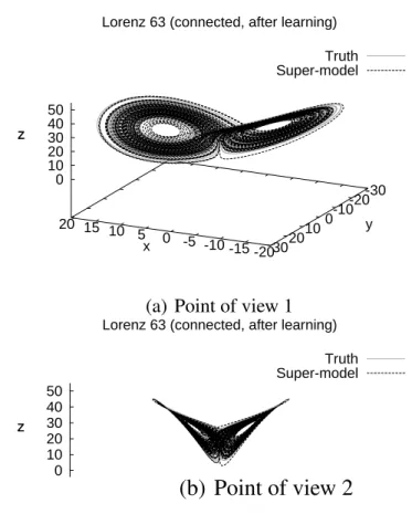
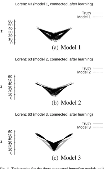
temporal correlations between thex,y, andzvariables of the three models are in excess of 0.95 (not shown) and the sum of the time-mean distances between the three model states normalized by the sum of the standard deviations ofxs, ys andzs is 0.34. In particular thez-values of the third model are systematically larger than those of the other two models (see Fig. 4). The improvement in the behaviour of the con-nected imperfect model solutions as depicted in Fig. 4 (to be compared with Fig. 2) is a clear indication of the feasibil-ity of super-modeling in the context of this low-dimensional chaotic system.
In addition to this minimum, we found that by choosing different initial values for the connection coefficients in the minimisation procedure different local minima in the cost function are obtained with values of the cost function that are of comparable magnitude. In the remainder of this section we will test the robustness of the learning process, research the issue of local minima and develop measures to determine the quality of the different super-model solutions.
-20 -15 -10 -5 0 5 10 15 20
-30 -20 -10 0 10 20 30 0
10 20 30 40 50 z
Lorenz 63 (connected, after learning) Truth Super-model
x
y z
(a) Point of view 1
0 10 20 30 40 50 z
Lorenz 63 (connected, after learning) Truth Super-model
z
(b) Point of view 2
Fig. 3. Trajectories for the super-model (black) and the standard Lorenz 63 system (grey) from two different points of view.
3.1 Robustness
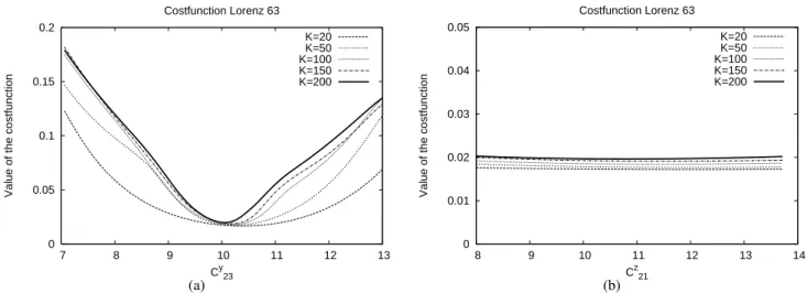
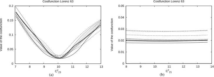
The minimum of the cost function is determined on a limited period of observations of length(K−1)·d+1that we refer to as the training set. We have chosenK= 200 to determine the minimum and subsequently evaluate the cost function us-ing theCvalues of this minimum for subsets of the training set of length corresponding toK= 20, 50, 100, 150. Cross sections of the cost function around the minimum can be cre-ated by changing one connection coefficient and keeping the others fixed at the values of the minimum. The cross sections for the different subsets are plotted in Fig. 5 for connection coefficientsC23y andC21z , since these are typical examples.
0 10 20 30 40 50 60 z
Lorenz 63 (model 1, connected, after learning) Truth Model 1
z
(a) Model 1
0 10 20 30 40 50 60 z
Lorenz 63 (model 2, connected, after learning) Truth Model 2
z
(b) Model 2
0 10 20 30 40 50 60 z
Lorenz 63 (model 3, connected, after learning) Truth Model 3
z
(c) Model 3
Fig. 4. Trajectories for the three connected imperfect models with connections determined by the learning process (black) and the standard Lorenz 63 system (grey).
of super-models of similar quality can be found by changing connection coefficientC21z between 8 and 14.
Ideally the super-model found by the learning process is not dependent on the training set. To test whetherK= 200 is large enough for this to be true the cost function is plotted in Fig. 6 for different periods of observations: the training set and independent sets of the same size that were obtained from a longer consecutive integration of the truth. Again the cross sections for connection coefficientsC23y and C21z are shown (Fig. 6). In Fig. 6a the position and value of the min-imum remain close to that of the training set. In Fig. 6b the cost function is flat for all sets of observations. We conclude that withK= 200 the cost function verifies rather well on in-dependent data, soK= 200 seems a reasonable size of the training set.
Table 2. The connection coefficients of two super-model solutions of the Lorenz 63 system and their differences.
Super-model 1 Super-model 2 Difference
C12x −0.01 1.52 1.53
C13x 4.81 0.03 −4.78
C21x 5.69 13.28 7.59
C23x 13.75 14.99 1.24
C31x 17.64 21.51 3.87
C32x −0.01 1.09 1.10
C12y 7.67 3.53 −4.14
C13y 18.14 27.36 9.22
C21y 3.64 0.00 −3.64
C23y 10.06 6.50 −3.56
C31y 2.71 3.89 1.18
C32y 9.79 6.93 −2.86
C12z 5.47 3.95 −1.52
C13z 4.03 12.24 8.21
C21z 10.72 3.50 −7.22
C23z 13.54 2.20 −11.34
C31z 8.70 2.89 −5.81
C32z 1.50 3.85 2.35
3.2 Local minima
In the previous section we noted that there is a large fam-ily of super-model solutions with similar values of the cost function connected to the minimum found by the minimisa-tion. The minimisation was repeated starting from random values for the connection coefficients between [0, 10] that were drawn from a uniform probability distribution. In this way we found other minima that are distinct in many more connection coefficients. For one of these minima, the con-nection coefficients are shown in Table 2, together with the values for the first minimum. In the fourth column the differ-ence between the connection coefficients of minima 1 and 2 indicates that the minima are clearly distinct and do not be-long to the same family of solutions.
A plot of the attractor of the second super-model solu-tion in its phase space (not shown) looks almost exactly the same as the plots of the first super-model solution in Figs. 3 and 4. The value of the cost function for the second solution is slightly lower (0.003 instead of 0.02) and is a first indi-cation that the second solution might be better. In the next section we will use various measures to evaluate the quality of these two super-model solutions.
3.3 Quality measures
0 0.05 0.1 0.15 0.2
7 8 9 10 11 12 13
Value of the costfunction
Cy23 Costfunction Lorenz 63
K=20 K=50 K=100 K=150 K=200
(a)
0 0.01 0.02 0.03 0.04 0.05
8 9 10 11 12 13 14
Value of the costfunction
Cz21 Costfunction Lorenz 63
K=20 K=50 K=100 K=150 K=200
(b)
Fig. 5.Cross section of the cost function for the super-model of the Lorenz 63 system calculated for different subsets of the original training set that was based onK= 200 initializations. The subsets vary in the number of initializations, i.e.K= 20, 50, 100, 150. A cross sections is created by changing connection coefficientsC23y in(a)andC21z in(b)and keeping the other coefficients fixed at the values of the minimum found by the learning process using the training set.
Table 3.Mean, standard deviation (SD) and covariance for the three unconnected imperfect models of the Lorenz 63 system. The values for the first two models are calculated analytically. Statistics for model 3 are based on 500 runs of 5000 time units. Between brackets the 95 % error estimation is given.
Model 1 Model 2 Model 3
Meanx ±7.94 ±7.93 0.003 (0.002)
Meany ±7.94 ±7.93 0.003 (0.010)
Meanz 18.00 17.00 34.23 (0.030)
SDx 0 0 7.628 (0.002)
SDy 0 0 9.416 (0.010)
SDz 0 0 8.765 (0.030)
Cov.xy 0 0 58.19 (0.036)
Cov.xz 0 0 0.007 (0.44)
Cov.yz 0 0 0.012 (0.68)
the quality of the super-model beyond the range that is in-fluenced by the initial conditions, different measures can be used as in climate simulations.
The most straightforward measures are the different mo-ments of the probability density function of the states in phase space, such as the mean, variance and covariance of the state variables. Since these do not take into account the temporal evolution through phase space, we will also evalu-ate the ability of the super-model to reproduce the autocorre-lation functions of the state variables. As a final measure we will check the ability of the super-model to synchronize with the truth at the end of this section.
Table 4.Mean, standard deviation (SD) and covariance for the truth and for the two super-models of the Lorenz 63 system. Statistics are based on 500 runs of 5000 time units. Between brackets the 95 % error estimation is given.
Truth Super-model 1 Super-model 2
Meanx −0.006 (0.22) 0.007 (0.21) −0.000 (0.25)
Meany −0.006 (0.22) 0.007 (0.21) −0.000 (0.25)
Meanz 23.549 (0.02) 22.93 (0.02) 23.19 (0.03)
SDx 7.924 (0.005) 7.717 (0.003) 7.812 (0.005)
SDy 9.011 (0.008) 8.791 (0.009) 8.723 (0.009)
SDz 8.623 (0.025) 8.596 (0.016) 8.549 (0.032)
Cov.xy 62.786 (0.07) 58.952 (0.05) 60.6416 (0.08)
Cov.xz −0.020 (0.76) 0.023 (0.74) 0.000 (0.88)
Cov.yz −0.016 (0.61) 0.021 (0.65) −0.001 (0.69)
Mean, standard deviation and covariance
The calculation of these statistics is based on 500 runs of 5000 time units of the truth, the imperfect models and both super-models. An error estimation of these quantities is based on the spread of the 500 estimates of each quantity. The results for the imperfect models are given in Table 3 and for the truth and both super-models in Table 4.
0 0.05 0.1 0.15 0.2
7 8 9 10 11 12 13
Value of the costfunction
Cy23 Costfunction Lorenz 63
(a)
0 0.01 0.02 0.03 0.04 0.05
8 9 10 11 12 13 14
Value of the costfunction
Cz21 Costfunction Lorenz 63
(b)
Fig. 6.As in Fig. 5, except that the cost function is calculated for the training set withK= 200 initializations (thick line) and 9 additional independent sets of observations of the same length (thin lines) that were taken from a consecutive longer integration of the truth.
The statistics of the chaotic solution of model 3 (see Table 3) differ substantially from the truth (see Table 4), especially the mean value ofzis much larger.
Both super-models (see Table 4) have statistics that are close to that of the truth with the largest differences of order 5 % in the covariance betweenx andy. The second super-model is somewhat closer to the truth, especially in the co-variance ofxandy.
3.4 Autocorrelation
The autocorrelation is a statistical measure of the temporal evolution. It gives an indication of the memory and time scales present in a system. The plots in Fig. 7 are based on 100 runs of 3000 time units and the shading corresponds to the 95 % error range of the autocorrelation of the truth.
Both super-models capture the fast decorrelation ofx and yand the slow decorrelation ofzwell, but the second super-model is closer to the truth. It also better represents the domi-nant time scale which is most apparent in the autocorrelation of z. After 9 oscillations super-model 1 runs out of phase with the truth somewhat, whereas super-model 2 is still in phase.
3.5 Synchronization with the truth
Pecora and Carroll (1990) have shown that limited informa-tion exchange between two identical Lorenz systems can lead to synchronization of the model states even when the systems are initialized from very different initial conditions and differ slightly in parameter values. The ability to synchronize with the truth is another measure of the quality of a model. In this section we will compare how well the super-models compare to a perfect model in this respect.
Yang et al. (2006) extended the study of synchro-nized Lorenz systems, re-interpreted in the context of data
assimilation. Following Yang et al. (2006) we add a so-called simple nudging term to the equations of they variable for each of the three connected imperfect models as in Eqs. (5). This term “nudges” the actual values ofyk to the observed valueyoand the value of parameterndetermines the strength of the nudging.
˙
xk =σk (yk −xk) + X
j6=k
Ckjx xj − xk
˙
yk =xk(ρk−zk) −yk+ X
j6=k
Ckjy yj−yk+n(yo−yk) (5) ˙
zk =xk yk −βkzk + X
j6=k
Ckjz zj −zk k = 1,2,3 We take the following definition of synchronization:
Definition 1 A model is synchronized with the truth if the RMS difference between the model state and observed true state att=t0is smaller thanδ and remains smaller thanǫ fort→ ∞.
ǫis chosen larger thanδ, since synchronized systems of-ten deviate somewhat during short extreme excursions of the trajectory, but remain synchronized. As a measure of syn-chronization we use the minimum strength of the nudging nfor which synchronization is accomplished independent of the initial condition, for integern. For practical purposes we choose a time interval ofT= 1000 time units during which the models must remain withinǫdistance of each other.
-0.2 -0.1 0 0.1 0.2 0.3 0.4 0.5
0 0.5 1 1.5 2 2.5 3 3.5 4
Autocorrelation
Time
Autocorrelation Lorenz 63 (x) 95% errorband
Truth Super model 1 Super model 2
(a)
x
-0.2 -0.1 0 0.1 0.2 0.3 0.4 0.5
0 0.5 1 1.5 2 2.5 3 3.5 4
Autocorrelation
Time
Autocorrelation Lorenz 63 (y) 95% errorband
Truth Super model 1 Super model 2
(b)
y
-0.8 -0.6 -0.4 -0.2 0 0.2 0.4 0.6 0.8 1
0 2 4 6 8 10
Autocorrelation
Time
Autocorrelation Lorenz 63 (z) Truth Super model 1 Super model 2
(c)
z
Fig. 7. Autocorrelation as a function of delay time forx, y and
zfor the standard Lorenz 63 system and both super-models. The shaded area indicates the 95 % error band for the autocorrelation of the truth, based on 100 runs of 3000 time units.
0 1 2 3 4
0 0.5 1 1.5 2 2.5 3 3.5 4
Probability Density
Distance PDF of distances for n=6
Copy of truth Super model 1 Super model 2
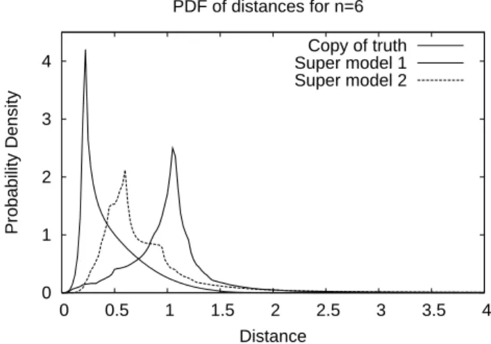
Fig. 8. Probability density function of the distance between the truth and the models while nudging the models to the truth in the
y-variable with strength n= 6. Plots are for a copy of the truth (thin solid), the first (thick solid) and the second super-model (thick dashed). The PDF is calculated from a simulation of length 105time units and is normalized to one.
a nudging strength of n= 11 in order to synchronize with the truth. The second super-model needs a somewhat larger valuen= 13. Using the same experimental setup, we found that the imperfect models individually are not able to syn-chronize with the truth at all. Both super-models need a stronger nudging than the perfect model. In this measure, the first super-model is closer to the truth, despite the fact that the mean temporal evolution, as measured by the auto-correlation, is more faithfully captured by the second super-model that also has a smaller cost function value. However, if we calculate the probability density function of the dis-tance between the truth and the super-model from a 105time units long integration of the super-model nudged to the truth as in Eqs. (5) forn= 6, we find that more often the second model remains closer to the truth than the first super-model (see Fig. 8). Nevertheless, the second super-super-model needs a slightly larger nudging strength to synchronize with the truth than the first because for nudging values larger than n= 5, it has larger probability, albeit small, of exceeding the thresholdǫ= 4. Forn= 6 the distance between the second super-model and the truth is larger than 4 during 1.6 % of the time whereas it is 1.3 % for the first. Forn= 10 it is 0.27 % for the second and 0.075 % for the first. This probability be-comes small enough to meet the synchronization criterium of Definition 1 forn= 13 for the second super-model, whereas for the first this happens forn= 11. We conclude that the interpretation of the ability of a model to synchronize with the truth as a measure of the quality of a solution is not so straightforward. It serves more as a measure of the stability of the model.
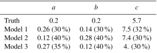
Table 5.Standard and perturbed parameters for the R¨ossler system.
a b c
Truth 0.2 0.2 5.7
Model 1 0.26 (30 %) 0.14 (30 %) 7.5 (32 %)
Model 2 0.12 (40 %) 0.28 (40 %) 7.4 (30 %)
Model 3 0.27 (35 %) 0.12 (40 %) 4. (30 %)
of the cost function is indeed a good indication of the quality of the solution and that the approach of minimizing the cost function is a fruitful strategy.
3.6 Simulating climate change
In order to check whether the super-model is also able to sim-ulate climate change, for instance the response of the truth to a parameter perturbation, we doubled the parameterρin the true system and in the imperfect models in the super-model. The response of the attractor is an increase in size, the shape remains very similar (see Fig. 9). Although the connection coefficients are learned forρ= 28, the super-model quite ac-curately simulates the attractor forρ= 56. The meanz-value increases with a factor of 2.2 for both the truth as well as the super-model. The response is practically the same for both super-models.
4 Results R¨ossler and Lorenz 84
In this section the super-modeling approach is applied to the R¨ossler and the Lorenz 84 systems. Both display chaotic behaviour for standard parameter settings, but the attractors are quite different.
4.1 R¨ossler
The Lorenz 63 attractor is also called a butterfly, because of its shape. As a simplification of this example of chaos to one where the attractor only has one “wing”, the R¨ossler equations were proposed (R¨ossler, 1976). The time evolution is less chaotic than in the Lorenz 63 system, since it lacks the irregular transitions between two unstable points. The equations are
˙
x= −(y +z) ˙
y=x +ay (6)
˙
z=b +z (x −c).
The parameter values for the truth are R¨osslers values: a= 0.2, b= 0.2 and c= 5.7. The values for the parameters for the three imperfect models can be found in Table 5. The parameter perturbations applied are again of the order 30 % to 40 % and in each of the imperfect models parameters have been decreased as well as increased.
0 20 40 60 80 100
z
Lorenz 63 (response after learning)
Truth Super-model True response Super-model response
z
Fig. 9.Trajectories for the second super-model (black) and the stan-dard Lorenz 63 system (grey). The larger attractor corresponds to
ρ= 56, the smaller to the standard valueρ= 28. The super-model was trained on the standard parameter value.
With these parameter perturbations marked changes occur in the attractor as can be seen in Fig. 10. The attractor of imperfect model 1 is still chaotic and has a similar shape but the amplitude of the irregular oscillations is larger. Imperfect model 2 and 3 have a periodic attractor of different shapes.
To determine the super-model we first need to choose val-ues for the different parameters in the cost function. For the R¨ossler system the time it takes for initial errors to double is on average 6.7. Following the same procedure as for the Lorenz 63 system we setγ= 0.9 and1= 12 time units. The number of initializations in this case isK= 300.
We minimized the cost function by varying the connection coefficients of the super-model. This minimum is plotted in Fig. 11 in a cross section alongC23x . The value at the min-imum is approximately 0.0001, which is much lower than a typical value of the cost function (0.004 for all connec-tion coefficients equal to 1). To check the robustness of this minimum with respect to the limited size of training set, we calculated the cost function for 9 additional sets of 300 ini-tializations, that were taken from a longer simulation of the truth. The figure shows that 300 initializations are enough to reliably estimate the cost function. This minimum is not unique. By changing the initial values of the connection co-efficients in the minimisation procedure, we found different minima with similar values of the cost function as was the case for the Lorenz 63 system. Here we evaluate the quality of this minimum only.
-15 -10 -5 0 5 10 15 20 -20
-15 -10 -5 0 5 10 15
0 10 20 30 40 50 60 70 80
z
Rossler (model 1, unconnected) Truth Model 1
x y
z
(a) Model 1
-10 -5 0 5 10 15 -15
-10 -5 0 5 10
0 5 10 15 20 25 30 35
z
Rossler (model 2, unconnected) Truth Model 2
x y
z
(b) Model 2
-10 -5 0 5 10 15 -15
-10 -5 0 5 10
0 5 10 15 20 25 30 35
z
Rossler (model 3, unconnected) Truth Model 3
x y
z
(c) Model 3
Fig. 10. Trajectories for the three unconnected imperfect models (black) and the standard R¨ossler system (grey). Note the different scales on the axes. The truth is the same in all three plots.
Table 6.Mean, standard deviation (SD) and covariance for the three unconnected imperfect models of the R¨ossler system. The 95 % er-ror estimation based on 500 runs of 5000 time units is given between brackets.
Model 1 Model 2 Model 3
Meanx 0.417 (0.082) 0.085 (0.0009) 0.34 (0.0009) Meany −1.603 (0.099) −0.710 (0.0009) −1.26 (0.0009) Meanz 1.603 (0.230) 0.710 (0.0015) 1.26 (0.0022) SDx 6.759 (0.082) 6.659 (0.0009) 4.463 (0.0008) SDy 6.567 (0.099) 6.400 (0.0009) 4.080 (0.0009) SDz 6.853 (0.229) 1.787 (0.0015) 3.896 (0.0022) Covariancexy -11.21 (0.33) −4.492 (0.005) −4.49 (0.004) Covariancexz 11.21 (0.33) 4.916 (0.006) 4.49 (0.004) Covarianceyz -0.35 (0.39) 2.784 (0.004) 2.06 (0.003)
0 0.0001 0.0002 0.0003 0.0004 0.0005 0.0006 0.0007 0.0008
1 1.5 2 2.5 3 3.5 4 4.5
Value of the costfunction
C23x Rossler, Costfunction
Fig. 11. Cross sections of the cost function for the super-model of the R¨ossler system for the training set (thick line) with length corresponding toK= 300 and 9 additional independent sets of the same length (thin lines). Cross sections are created by changing the connection coefficientC23x and keeping the others fixed.
is very similar to the true attractor. We will apply the same measures as for the Lorenz 63 system to check the quality of the super-model.
First we compare the means, standard deviations and co-variances for the unconnected imperfect models in Table 6 and for the model and the truth in Table 7. The super-model turns out to be closer to the truth than the best im-perfect model (model 3). Its statistics almost fall within the 95 % error bounds of the true values.
-10 -5 0 5 10 15 -12
-10-8 -6 -4 -2 0 2 4 6 8 0 5 10 15 20 25 30 35
z
Rossler, after learning
Truth Model 1
x y
z
(a) Model 1
-10 -5 0 5 10 15 -12
-10-8 -6 -4 -2 0 2 4 6 8 0 5 10 15 20 25 30 35
z
Rossler, after learning
Truth Model 2
x y
z
(b) Model 2
-10 -5 0 5 10 15 -12
-10-8 -6 -4 -2 0 2 4 6 8 0 5 10 15 20 25 30 35
z
Rossler, after learning
Truth Model 3
x y
z
(c) Model 3
Fig. 12.Trajectories for the three connected imperfect models with connections determined by the learning process (black) and the standard R¨ossler system (grey).
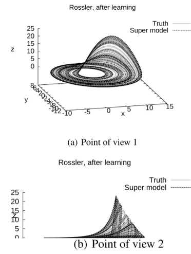
-10 -5 0 5 10 15 -12
-10-8 -6 -4 -2 0 2 4 6 8 0 5 10 15 20 25
z
Rossler, after learning
Truth Super model
x y
z
(a) Point of view 1
0 5 10 15 20 25
z
Rossler, after learning
Truth Super model
z
(b) Point of view 2
Fig. 13. Trajectories for the super-model (black) and the standard R¨ossler system (grey) for two different points of view.
Finally we look at the minimum nudging strength needed to enable synchronization with the truth. We use the same definition of synchronization as for the Lorenz 63 model with the following values for the parametersδ= 0.05,ǫ= 0.4 and T= 1000 time units. When the nudging term is applied to the yvariable only, we find that the standard R¨ossler system syn-chronizes with a copy of itself for a nudging strength equal ton= 1. The super-model also synchronizes when nudging only they variable, but it needs a stronger nudging ofn= 2. It outperforms model 3 in this measure; even by replacing the yvariable with the true value (which corresponds effectively to an infinitely large nudging strength), synchronization does not occur.
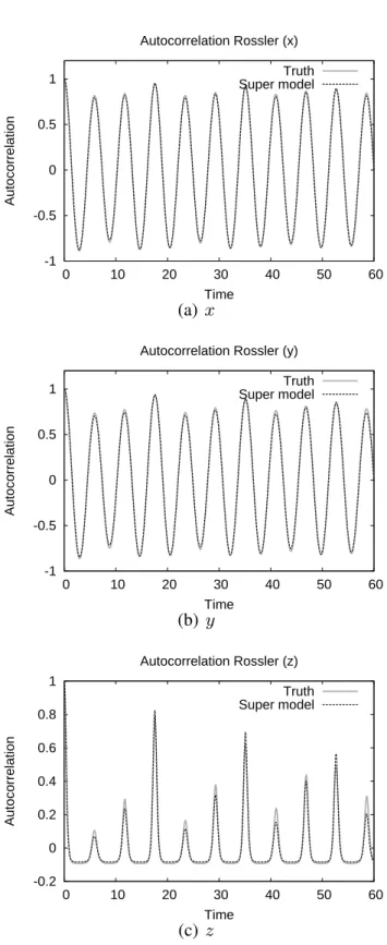
-1 -0.5 0 0.5 1
0 10 20 30 40 50 60
Autocorrelation
Time
Autocorrelation Rossler (x) Truth Super model
(a)
x
-1 -0.5 0 0.5 1
0 10 20 30 40 50 60
Autocorrelation
Time
Autocorrelation Rossler (y) Truth Super model
(b)
y
-0.2 0 0.2 0.4 0.6 0.8 1
0 10 20 30 40 50 60
Autocorrelation
Time
Autocorrelation Rossler (z) Truth Super model
(c)
z
Fig. 14. Autocorrelation for the super-model (black) and the stan-dard R¨ossler system (grey). The thickness of the grey line corre-sponds to the 95 % error band for the truth, based on 100 runs of 3000 time units.
Table 7.Mean, standard deviation (SD) and covariance for the truth and super-model of the R¨ossler system. The 95 % error estimation based on 500 runs of 5000 time units is given between brackets.
Truth Super-model
Meanx 0.177 (0.003) 0.175 (0.003)
Meany −0.886 (0.009) −0.878 (0.009)
Meanz 0.886 (0.009) 0.874 (0.009)
SDx 5.16 (0.04) 5.10 (0.03)
SDy 4.84 (0.03) 4.82 (0.02)
SDz 2.84 (0.04) 2.95 (0.03)
Covariancexy −4.693 (0.05) −4.702 (0.04)
Covariancexz 4.693 (0.05) 4.644 (0.04)
Covarianceyz 2.183 (0.12) 2.025 (0.19)
more chaos helps or hurts, so we test the super-modeling ap-proach also on the more chaotic Lorenz 84 system.
4.2 Lorenz 84
The Lorenz 84 system was proposed by Lorenz as a toy model for the general atmospheric circulation at midlatitudes (Lorenz, 1984). The model equations are
˙
x = −y2 −z2 −ax +aF
˙
y =xy −bxz− y +G (7)
˙
z=bxy +xz− z.
The x variable represents the intensity of the globe-encircling westerly winds andy andzrepresent a travelling large-scale wave that interacts with the westerly wind. Pa-rametersF andGare forcing terms representing the average north-south temperature contrast and the east-west asymme-tries due to the land-sea distribution respectively.
The standard parameter values for the truth area=14,b= 4, F= 8 and G= 1, for which the model displays chaotic be-haviour (van Veen, 2001). In Table 8 the perturbed parameter values of the imperfect models are given. The perturbations are again about 30 % and in each imperfect model parameters have been decreased as well as increased.
With these parameter perturbations the attractor of the imperfect models differs substantially from the truth (see Fig. 15). Both model 1 and 3 have periodic attractors, whereas model 2 has a point attractor (the transient evolu-tion towards the point attractor is shown for model 2). The periodic behaviour corresponds to the wave traveling period-ically around the hemisphere.
-1 -0.5 0 0.5 1 1.5 2 2.5 -2
-1 0
1 2 -2
-1 0 1 2 3
z
Truth Model 1
x y
z
(a) Model 1
-1 -0.5 0 0.5 1 1.5 2 2.5 -2
-1 0
1 2 -2
-1 0 1 2 3
z
Truth Model 2
x y
z
(b) Model 2
-1 -0.5 0 0.5 1 1.5 2 2.5 -2
-1 0
1 2 -2
-1 0 1 2 3
z
Truth Model 3
x y
z
(c) Model 3
Fig. 15. Trajectories for the three unconnected imperfect models (black) and the standard Lorenz 84 system (grey).
Table 8.Standard and perturbed parameters for the Lorenz 84 sys-tem.
a b F G
Truth 0.25 4 8 1
Model 1 0.33 (32 %) 5.2 (30 %) 10.4 (30 %) 0.7 (30 %) Model 2 0.18 (28 %) 5.2 (30 %) 5.6 (30 %) 1.3 (30 %) Model 3 0.18 (28 %) 2.7 (33 %) 10.4 (30 %) 1.3 (30 %)
0.0002 0.0003 0.0004 0.0005 0.0006 0.0007 0.0008 0.0009
4.5 5 5.5 6 6.5 7 7.5 8
Value of the costfunction
C32y Lorenz 84, Costfunction
Fig. 16. Cross section of the cost function for the super-model of the Lorenz 84 system for the training set (thick line) with length corresponding toK= 200 and 9 additional independent sets of the same length (thin lines). Cross sections are created by changing the connection coefficientC32y and keeping the others fixed.
autocorrelation function ofx(0.6 at 8 time units, see Fig. 18) indicates that the initial conditions still have an impact on the evolution after 8 time units. Therefore we decided to in-crease1to 8 andγ to 0.8. In addition it turned out that it was easier to find good minima using the amoeba minimisa-tion algorithm (Nelder and Mead, 1965) instead of the con-jugate gradients minimisation. The amoeba method does not need gradient information and is less susceptible to getting stuck in local minima. The training set is based onK= 200 initializations, each 0.2 time units apart selected from a long simulation of the truth.
-1 -0.5 0 0.5 1 1.5 2 2.5 -2.5
-2-1.5 -1-0.5
0 0.5 1
1.5 2 2.5 -2.5-2
-1.5-1 -0.5 0 0.5 1 1.5 2 2.5
z
Truth Supermodel
x y
z
(a) Point of view 1
-2.5-2 -1.5-1 -0.5 0 0.5 1 1.5 2 2.5
z
Truth Supermodel
z
(b) Point of view 2
Fig. 17. Trajectories for the super-model (black) and the standard Lorenz 84 system(grey) for two points of view.
With the connection coefficients for this minimum, we in-tegrated the super-model and plotted the trajectory in Fig. 17. A visual comparison with the truth indicates a very good agreement. In this case the three imperfect models are almost perfectly synchronized (not shown). The synchronization is stronger in this case as compared to the other two systems. The temporal correlations between thex,yandzvariables of the three imperfect models in the super-model are in excess of 0.99 and the sum of the time-mean distances between the three model states normalized by the sum of the standard de-viations ofxs,ys andzsis only 0.03. The model trajectories stay very close together on average. The reason for this might be found in the high value of several connection coefficients (for instanceC32x = 115,Cy23= 147 andC31z = 169). Such high values make synchronization easier since these connection terms in the equations bring the model solutions closer to-gether. Maximum values of the connection coefficients in the other two systems are a factor of 10 smaller.
Again we use the same measures to evaluate the quality of the super-model solution. The mean, standard deviation and covariance for the truth and the super-model are presented in Table 9. These statistics are in excellent agreement.
In order to evaluate the temporal behaviour we compare the autocorrelation functions in Fig. 18. Up to a delay time of 14 time units the autocorrelation functions of the truth are
Table 9. Mean, standard deviation (SD) and covariance for the super-model and the standard Lorenz 84 system. The 95 % error estimation based on 500 runs of 5000 time units is given between brackets.
Truth Super-model
Meanx 1.015 (0.008) 1.013 (0.008)
Meany 0.060 (0.018) 0.058 (0.017)
Meanz 0.271 (0.005) 0.272 (0.004)
SDx 0.589 (0.014) 0.596 (0.014)
SDy 0.919 (0.002) 0.920 (0.002)
SDz 0.908 (0.002) 0.906 (0.002)
Covariancexy −0.053 (0.018) −0.050 (0.022) Covariancexz −0.038 (0.004) −0.039 (0.003) Covarianceyz −0.075 (0.006) −0.063 (0.005)
well reproduced by the super-model both in shape as well as in periodicity.
The Lorenz 84 system with standard parameter values synchronizes with the truth for a strength of the nudging termn=1 in they variable only, usingδ= 0.1,ǫ= 0.5 and T= 1000 in Definition 1. The super-model also synchronizes with the truth, but it needs a larger nudging ofn= 4. None of the imperfect models is able to synchronize with the truth, when the nudging is in theyvariable only.
Concluding this section, super-model solutions can be found that reproduce the true system very well and outper-form the individual imperfect models for the Lorenz 84 sys-tem as well. For this syssys-tem, the minimisation process was found to be more sensitive to the length of the short integra-tions1and the discount parameter γ, requiring the use of the more robust amoeba minimisation procedure.
5 Conclusion and discussion
In this study we developed and tested a novel multi-model ensemble approach in which imperfect models of an ob-servable system are combined into a single super-model by letting the models exchange information during the simula-tion. The information exchange takes the form of linear con-nections with weights that are learned from historical data such that the supmodel minimizes the mean squared er-rors in short simulations initialized from past observed states. The main result of this study is that it is possible to con-struct super-models in the context of simple low-dimensional chaotic systems that outperform the constituent imperfect models.
-0.6 -0.4 -0.2 0 0.2 0.4 0.6 0.8 1
0 5 10 15 20
Autocorrelation
Time
Autocorrelation Lorenz 84 (x) 95% errorband
Truth Model
(a)
x
-0.4 -0.3 -0.2 -0.1 0 0.1 0.2 0.3 0.4
0 2 4 6 8 10 12 14
Autocorrelation
Time
Autocorrelation Lorenz 84 (y) 95% errorband
Truth Model
(b)
y
-0.4 -0.3 -0.2 -0.1 0 0.1 0.2 0.3 0.4
0 2 4 6 8 10 12 14
Autocorrelation
Time
Autocorrelation Lorenz 84 (z) 95% errorband
Truth Model
(c)
z
Fig. 18. Autocorrelation for the super-model (black) and the stan-dard Lorenz 84 system (white) The shaded area corresponds to the 95 % error band for the truth based on 100 runs of 3000 time units.
model uncertainty, the outcomes of the different models are combined into a single estimate of the probability density function of climate variables. This study indicates that better estimates of the true probability function can be obtained if the models are taught, using past observations, to combine the strengths of each into a single forecast of the probability density function.
In case the models synchronize perfectly, all models fol-low the same trajectory and no information is lost by en-semble averaging. A sudden loss of synchronization and in-crease of spread between the individual model solutions in the super-model might indicate a loss of predictability dur-ing that period. Also, the distance from the ensemble mean might be an indication of model error, the larger the distance, the larger the model error. We note that, since the models are coupled (rather than independent), the super-model is not an ensemble in the classical sense of probability theory. But in addition to evaluating the ensemble mean, valuable informa-tion might be obtained from the spread between the individ-ual model realizations.
A large gap exists between the simple, chaotic systems of this study and the complex, state-of-the-art climate models. Many questions need to be addressed in order to apply the same approach to these models. There is the practical limita-tion of computer capacity to enable the parallel execulimita-tion of an ensemble of state-of-the-art models that need to exchange information at every time step. In the study of Kirtman et al. (2003) two atmospheric models were coupled to one ocean model so in principle it should be feasible to couple sev-eral atmospheric models to sevsev-eral ocean models. Compu-tational grids in the various climate models differ, so regrid-ding should be part of the information exchange. Regridregrid-ding is standard practice in the information exchange between the atmosphere and ocean components of climate models.
The introduction of connections between models intro-duces non-physical terms in the equations and might dis-rupt physical balances present in the original equations. On the true climate attractor, the physical balances are natu-rally obeyed. In case the models synchronize with the ob-servations and each other, the physical balances are obeyed also, and the precise implementation of the connections does not matter. With regard to the approximate balances that are observed in the atmosphere, like the hydrostatic or the geostrophic balance, we note that if the connections be-tween the state variables remain sufficiently weak, these bal-ances will be restored continuously by dynamical adjust-ments within each individual model.
An additional complicating factor for the learning phase is the difference in time-scale between atmosphere and ocean. Adjustments in the atmosphere have a short time-scale, but the ocean adapts to these changes on a much longer time-scale. Through its influence on the atmosphere, the ocean introduces longer time-scales in the atmosphere as well. So short integrations during the learning phase do not probe these effects. This might hamper the learning. On the other hand, there are well documented examples that certain model errors develop very quickly. Rodwell and Jung (2008) is an example of how a particular model error, namely the amount of aerosols over the Sahara, leads to remote biases in winds and precipitation through a sequence of fast atmospheric pro-cesses. It is a nice example of how difficult it can be to di-agnose the origin of a particular model bias. But at the same time it illustrates that model biases develop quickly and it im-plies that improving climate models on the short time-scales (as in the super-model approach) could be a fruitful approach to reduce model biases. Jung (2005) shows that most of the climatogical errors in the circulation are already developed after ten days of integration when starting from observed states. In addition in Jung et al. (2009) it is reported that a change in the deep convection scheme, which describes fast turbulent processes on the time-scales of hours, led to a marked reduction of the climatological model bias. See further Palmer and Weisheimer (2010) for a more theoretical view on the origin of systematic model errors.
A main result of this study is that super-model solutions are not unique. However, the different super-models have similar quality and therefore this does not pose a severe prob-lem and makes finding a suitable super-model solution easier. The existence of quite distinct super-model solutions of good quality remains a bit of a mystery.
A hierarchy of earth system models of intermediate com-plexity (EMIC’s) could be used to address these various is-sues. The EMIC’s resemble the state-of-the-art climate mod-els in their structure, but differ in that the parameterization schemes for the physical processes are much less elaborate, fewer processes are explicitly modeled and the spatial res-olution is much coarser. It has already been demonstrated that two different quasi-geostrophic channel models will syn-chronize with only limited connections (Duane and Tribbia,
2001, 2004). A fruitful strategy might be to start from a rel-atively simple climate model and add to the complexity in small steps and address a specific issue at each step. In a sim-ilar fashion as in this study a ground truth model is assumed at each step and an ensemble of imperfect models is created by perturbing parameters and/or using different formulations for unresolved processes.
An alternative learning strategy that is explicitly based on synchronization is outlined in the study by Duane et al. (2007). In this strategy the super-model equations contain nudging terms to the truth as in our Eqs. (5) and additional evolution equations are formulated for the parameters. The moment the super-model synchronizes with the truth the pa-rameters stop updating. This alternative learning strategy leads to a particularly simple learning law that could be use-ful in the implementation of the super-model approach us-ing more complex models. The strategy has been demon-strated with Lorenz systems (Duane et al., 2009). Quinn et al. (2009) present a learning strategy based on the minimisa-tion of a similar cost funcminimisa-tion by varying parameters and the initial state of a single model simulation with an additional nudging term to the truth that allows the model to synchro-nize with the truth during the learning. In this sense it re-sembles the approach by Duane et al. (2007). Our approach is different in that we consider an ensemble of short model simulations from different initial states, do not nudge to the truth and only vary the parameters and not the initial state to minimize the cost function.
The main caveat is that the super-model is trained on his-torical data and in a climate prediction problem is subse-quently applied to simulate the response of the system to an external forcing. It is not guaranteed that the super-model will also simulate this response more realistically, since the response was not part of the training. Therefore the super-model approach is more likely to be successful in weather-and seasonal predictions since the cases to be predicted re-main closer to the cases present in the training set.
The problem is not peculiar to the super-modeling ap-proach, but arises with climate models generally. Climate models contain numerous empirical parameters with values that are optimized to reproduce observed historical behav-ior as close as possible. Parameter values are adjusted such as to reduce the errors in the climatological mean fields using historical observations (Severijns and Hazeleger, 2005; Med-vigy et al., 2010). It is not guaranteed that this automatically implies that the response to a future greenhouse gas forcing will be simulated more realistically. Other processes might play a role there (Klocke et al., 2011).
climate models will help in improving predictions of the cli-mate response to future greenhouse gas forcing.
To conclude, as argued above, the super-modeling ap-proach might work or might fail in the context of complex climate models. This remains to be seen. We propose to fur-ther study the merits of the super-modeling approach using a similar hypothetical model setting as in this paper with a hypothetical perfect model simulating the truth and a set of imperfect models simulating state-of-the-art approximations of this hypothetical truth. For this super-modeling research, model classes of increased complexity – both for the hypo-thetical truth as for the imperfect model approximations – are then to be explored.
Finally, we wish to stress that we believe that long-term improvements in climate predictions must come from im-proving the description of the physical processes on the ba-sis of dedicated process studies and observational databases. This is a slow, but necessary process. In the meanwhile, given a set of imperfect models, we could try to improve pre-dictions by combining the strengths of the individual models either through multi-model or super-model approaches.
Acknowledgements. This work has been partially supported by FP7 FET Open Grant# 266722 (SUMO project) and DOE Grant# DE-SC0005238.
Edited by: A. Alessandri
References
Compo, G., Whitaker, J., and Sardeshmukh, P.: Feasibility of a 100-Year Reanalysis Using Only Surface Pressure Data, B. Am. Me-teorol. Soc., 87, 175–189, 2006.
Duane, G. and Tribbia, J.: Synchronized chaos in geophysical fluid dynamics, Phys. Rev. Lett., 86, 4298–4301, 2001.
Duane, G. and Tribbia, J.: Weak Atlantic-Pacific teleconnections as synchronized chaos, J. Atmos. Sci., 61, 2149–2168, 2004. Duane, G. S., Tribbia, J. J., and Weiss, J. B.: Synchronicity in
pre-dictive modelling: a new view of data assimilation, Nonlin. Pro-cesses Geophys., 13, 601–612, doi:10.5194/npg-13-601-2006, 2006.
Duane, G., Yu, D., and Kocarev, L.: Identical synchronization, with translation invariance, implies parameter estimation, Phys. Lett. A, 371, 416–420, 2007.
Duane, G., Tribbia, J., and Kirtman, B.: Consensus on Long-Range Prediction by Adaptive Synchronization of Models, EGU Gen-eral Assembly, Vienna, Austria, 2009.
Fletcher, R. and Reeves, C.: Function minimization by conjugate gradients, Comput. J., 6, 149–154, 1963.
IPCC: Climate Change 2007: The Physical Science Basis, Con-tribution of Working Group I to the Fourth Assessment Report of the Intergovernmental Panel on Climate Change, edited by: Solomon, S., Qin, D., Manning, M., Chen, Z., Marquis, M., Av-eryt, K. B., Tignor, M., and Miller, H. L., Cambridge University Press, Cambridge, UK and New York, USA, 2007.
Jung, T.: Systematic errors of the atmospheric circulation in the ECMWF forecasting system, Q. J. Roy. Meteorol. Soc., 131, 1045–1073, 2005.
Jung, T., Balsamo, G., Bechtold, P., Beljaars, A., K¨ohler, M., Miller, M., Morcrette, J.-J., Orr, A., Rodwell, M., and Tompkins, A. M.: The ECMWF model climate: Recent progress through im-proved physical parametrizations, available from the ECMWF website: http://ecmwf.intECMWF, last access: 29 June 2011, Seminar Proceedings on Parameterization of Subgrid-scale Pro-cesses, 233–249, 2009.
Kirtman, B., Min, D., Schopf, P., and Schneider, E.: A new ap-proach for CGCM sensitivity studies, COLA Technical Report, 154, 50 pp., 2003.
Klocke, D., Pincus, R., and Quaas, J.: On constraining estimates of climate sensitivity with present-day observations through model weighting, J. Climate, in press, doi:10.1175/2011JCLI4193.1, 2011.
Lorenz, E.: Deterministic Nonperiodic Flow, J. Atmos. Sci., 20, 130–140, 1963.
Lorenz, E.: Irregularity, a fundamental property of the atmosphere, Tellus A, 36, 98–110, 1984.
Medvigy, D., Walko, R. L., Otte, M. J., and Avissar, R.: The Ocean-Land-Atmosphere Model: Optimization and evaluation of simu-lated radiative fluxes and precipitation, Mon. Weather Rev., 138, 1923–1939, 2010.
Nelder, J. and Mead, R.: A simplex method for function minimiza-tion, Comput. J., 7, 308–313, 1965.
Palmer, T. N. and Weisheimer, A.: Diagnosing the Causes of Bias in Climate Models – Why it is so Hard?, available from the ECMWF website: http://ecmwf.int, last access: 29 June 2011, ECMWF Seminar Proceedings on Diagnosis of Forecasting and Data Assimilation Systems, 1–13, 2010.
Pecora, L. and Carroll, T.: Synchronization in Chaotic Systems, Phys. Rev. Lett., 64, 824–824, 1990.
Quinn, J. C., Bryant, P. H., Creveling, D. R., Klein, S. R., and Abar-banel, H. D. I.: Parameter and state estimation of experimental chaotic systems using synchronization, Phys. Rev. E, 80, 016201, doi:10.1103/PhysRevE.80.016201, 2009.
Rodwell, M. and Jung, T.: Understanding the local and global im-pacts of model physics changes: an aerosol example, Q. J. Roy. Meteorol. Soc., 134, 1479–1497, 2008.
R¨ossler, O.: An equation for continuous chaos, Phys. Lett. A, 75, 397–398, 1976.
Severijns, C. A. and Hazeleger, W.: Optimizing parameters in an at-mospheric general circulation model, J. Climate, 18, 3527–3535, 2005.
Tebaldi, C. and Knutti, R.: The use of the multi-model ensemble in probabilistic climate projections, Philos. T. Roy. Soc. A, 365, 2053–2075, 2007.
van Veen, L.: Active and passive ocean regimes in a low-order cli-mate model, Tellus A, 53, 616–628, 2001.