A multi-model ensemble method that combines imperfect models through learning

(1)

ESDD

1, 247–296, 2010

Combining imperfect models through

learning

L. A. Van den Berge et al.

Title Page

Abstract Introduction

Conclusions References

Tables Figures

◭ ◮

Back Close

Full Screen / Esc

Printer-friendly Version Interactive Discussion

Discussion

P

a

per

|

Dis

cussion

P

a

per

|

Discussion

P

a

per

|

Discussio

n

P

a

per

|

Earth Syst. Dynam. Discuss., 1, 247–296, 2010 www.earth-syst-dynam-discuss.net/1/247/2010/ doi:10.5194/esdd-1-247-2010

Earth System Dynamics Discussions

This discussion paper is/has been under review for the journal Earth System Dynamics (ESD). Please refer to the corresponding final paper in ESD if available.

A multi-model ensemble method that

combines imperfect models through

learning

L. A. van den Berge1, F. M. Selten1, W. Wiegerinck2, and G. S. Duane3

1

Royal Netherlands Meteorological Institute, Wilhelminalaan 10, 3732 GK, De Bilt, The Netherlands

2

Donders Institute for Brain, Cognition and Behaviour, Radboud University Nijmegen, Geert Grooteplein 21, 6525 EZ, Nijmegen, The Netherlands

3

Department of Atmospheric and Oceanic Sciences, University of Colorado, Boulder, CO 80309, USA

Received: 6 July 2010 – Accepted: 17 September 2010 – Published: 1 October 2010 Correspondence to: F. M. Selten ([email protected])

(2)

ESDD

1, 247–296, 2010

learning

Title Page

Tables Figures

◭ ◮

Back Close

Full Screen / Esc

Discussion

P

a

per

|

Dis

cussion

P

a

per

|

Discussion

P

a

per

|

Discussio

n

P

a

per

|

Abstract

In the current multi-model ensemble approach climate model simulations are com-bined a posteriori. In the method of this study the models in the ensemble exchange information during simulations and learn from historical observations to combine their strengths into a best representation of the observed climate. The method is devel-5

oped and tested in the context of small chaotic dynamical systems, like the Lorenz 63 system. Imperfect models are created by perturbing the standard parameter values. Three imperfect models are combined into one super-model, through the introduction of connections between the model equations. The connection coefficients are learned from data from the unperturbed model, that is regarded as the truth.

10

The main result of this study is that after learning the super-model is a very good approximation to the truth, much better than each imperfect model separately. These illustrative examples suggest that the super-modeling approach is a promising strategy to improve climate simulations.

1 Introduction

15

There is a broad scientific consensus that our climate is warming due to anthropogenic emissions of greenhouse gasses (IPCC, 2007). Due to the large impacts of climate change on society there is a growing need to widely sample and assess the possible climate change related to the plausible scenarios for future emissions. At about a dozen climate institutes around the world complex climate models have been developed over 20

the past decades. Despite the improvements in the quality of the model simulations, the models are still far from perfect. For instance a temperature bias of several degrees in annual mean temperatures in large regions of the globe is not uncommon in the simulations of the present climate (IPCC, 2007).

Nevertheless these models are used to simulate the response of the climate system 25

(3)

ESDD

1, 247–296, 2010

learning

Title Page

Tables Figures

◭ ◮

Back Close

Full Screen / Esc

Discussion

P

a

per

|

Dis

cussion

P

a

per

|

Discussion

P

a

per

|

Discussio

n

P

a

per

|

substantially in their simulation of the response: the global mean temperature rise varies by as much as a factor of 2 and on regional scales the response can be reversed, e.g. decreased precipitation instead of an increase. It is not clear how to combine these outcomes to obtain the most realistic response. The standard approach is to take some form of a weighted average of the individual outcomes (Tebaldi and Knutti, 2007), but 5

is this the best strategy?

We think we can do better by letting the models exchange information during the simulation instead of combining the results of the individual models afterwards. We propose to combine the individual models into one super-model by prescribing con-nections between the model equations. The connection coefficients are learned from 10

historical observations. This way the super-model learns to combine the strengths of the individual models in order to optimally reproduce the historical climate. Is this approach feasible?

An example of combining models successfully is found in the study by Kirtman et al. (2003) in which they coupled two different atmospheric models to one ocean model. 15

It turned out that the most realistic simulation in terms of the annual mean, annual cycle and interannual variability of sea surface temperatures over the tropical pacific was obtained by coupling the momentum fluxes from one model and the heat and fresh water fluxes from the other to the ocean model.

Another indication that this approach might be feasible is found in the practice of data 20

assimilation (Compo et al., 2006). It turns out that with a limited amount of information, the complete state of the atmosphere can be recovered. Synchronization in chaotic systems provides an explanation why this is at all possible, since linking chaotic sys-tems with a signal from one system to the other is known to lead to synchronization of their states (Pecora and Carroll, 1990; Duane et al., 2006). Therefore we expect 25

that in the super-modeling approach only limited information needs to be exchanged to effectively influence the combined behaviour of the imperfect models.

(4)

ESDD

1, 247–296, 2010

learning

Title Page

Tables Figures

◭ ◮

Back Close

Full Screen / Esc

Discussion

P

a

per

|

Dis

cussion

P

a

per

|

Discussion

P

a

per

|

Discussio

n

P

a

per

|

truth and create imperfect models by perturbing the parameter values. Three imperfect models are connected and combined into a super-model. The strength of the connec-tions are determined from data from the ground truth through a learning process. The learning process takes the form of the minimization of a cost function that measures the di_fference between the truth and the super-model during short integrations.

5

In Sect. 2 the form of the connections is introduced, followed by the introduction of the cost function and the minimisation method. The super-modeling approach is applied to the Lorenz 63, R ¨ossler and Lorenz 84 systems in Sects. 3 and 4. Discussion and conclusion of the method and ideas for improvement can be found in Sect. 5.

2 The super-modeling approach

10

To introduce the super-modeling approach we use the Lorenz 63 system (Lorenz, 1963). The Lorenz 63 system is often used as a metaphore for the atmosphere, because of its abrupt regime changes and unstable nature. The equations for the Lorenz 63 system are

˙

x₌σ(y−x) 15

˙

y ₌x(ρ−z)−y (1)

˙

z₌xy−βz.

The standard parameter values areσ₌10,β₌8₃ andρ₌28. Numerical solutions are obtained by a fourth order Runge-Kutta time stepping scheme, with a time step of 0.01.

2.1 Connecting imperfect models

20

(5)

ESDD

1, 247–296, 2010

learning

Title Page

Tables Figures

◭ ◮

Back Close

Full Screen / Esc

Discussion

P

a

per

|

Dis

cussion

P

a

per

|

Discussion

P

a

per

|

Discussio

n

P

a

per

|

˙

x_k₌σ_k(y_k−x_k)₊X

j6=k

Cx_kj(x_j−x_k)

˙

y_k₌x_k(ρ_k−z_k)−y_k₊X

j6=k

C_kjy (y_j−y_k) (2)

˙

z_k₌x_ky_k−β_kz_k₊X

j6=k

Cz_kj(z_j−z_k), k₌1,2,3,

wherek indexes the three imperfect models with perturbed parameter valuesσ_k,β_k

andρ_k andCx_kj,C_kjy andCz_kj are referred to as connection coefficients. 5

Each variable of each model is connected to the other two models. This gives two connection coe_fficients for each of the variables and a total number of 2×3×3₌18 con-nection coefficients. These 18 coefficients will be learned from data that sample the truth. The solution of the super-model, denoted by subscript s, is taken to be the average of the imperfect models

10

x_s₌1

3(x1+x2+x3)

y_s₌1

3(y1+y2+y3) (3)

z_s₌1

3(z1+z2+z3).

2.2 Cost function

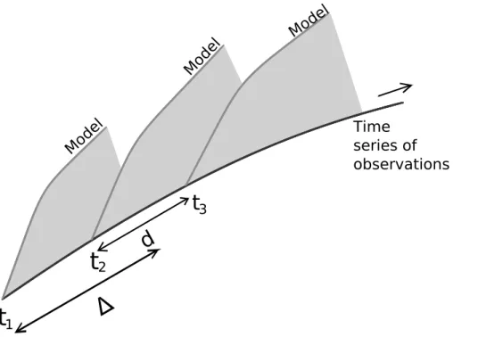
We assume that we have a long time series of observations of the truthx_o_{. We pick}

15

initial conditionsx

o(ti) from this long time series atK timesti,i=1,···,K, separated by

(6)

ESDD

1, 247–296, 2010

learning

Title Page

Tables Figures

◭ ◮

Back Close

Full Screen / Esc

Discussion

P

a

per

|

Dis

cussion

P

a

per

|

Discussion

P

a

per

|

Discussio

n

P

a

per

|

starting from theseK initializations (see Fig. 1). To measure the ability of the super-model to follow the truth we introduce the following cost functionF, that depends on the vector of connection coefficientsC_.

F(C₎₌ 1

K_∆

K X

i=1 Zti+∆

ti

|x

s(C,t)−xo(t)|2γtd t (4)

The cost function is normalized by _K1_∆, so that it represents the time averaged mean 5

squared error. The factorγt with 0<γ≤1 is introduced to give stronger weight to the errors close to the initial conditions. The idea behind this is that the Lorenz 63 system displays sensitive dependence on initial conditions. Trajectories diverge not only due to model imperfections, but also due to internal error growth: even a perfect model deviates from the truth if started from slightly different initial conditions and leads to 10

a non-zero cost function due to chaos. This implies that the cost function measures a mixture of model errors and internal error growth. Model errors dominate the inital divergence between model and truth, but at later times internal error growth dominates. Since we wish to measure the model errors, the factorγt discounts the errors at later times to decrease the contribution of internal error growth.

15

We base the choice of γ on the doubling time of errors. From a large number of runs (107) from randomly perturbed initial conditions we estimate the average doubling time τ of the initial error. We choose γ such that γτ₌1₂, so at time τ the weight is reduced to 1₂. For the Lorenz 63 systemτ₌0.75, which givesγ₌0.4. The length of the short integrations is taken to be_∆=1, which is a little bit longer than the doubling time. 20

By comparison the average time for one rotation in the Lorenz 63 system is 0.8. The separationd between the initializations is 0.2 time units.

2.3 Minimisation

For a fixed choice of the number of initializations K the cost function solely depends on the connection coefficients C _{in Eq. (4). The super-model can be determined by}

(7)

ESDD

1, 247–296, 2010

learning

Title Page

Tables Figures

◭ ◮

Back Close

Full Screen / Esc

Discussion

P

a

per

|

Dis

cussion

P

a

per

|

Discussion

P

a

per

|

Discussio

n

P

a

per

|

finding a minimum in the cost function in the 18 dimensional space ofC_{. For this we}

employ the Fletcher-Reeves-Polak-Ribiere Conjugate Gradient method (Fletcher and Reeves, 1963). It uses the gradient of the cost function to approach minima and stops when the gradient is (close to) zero.

We found it advantageous to make use of the dependence of the cost function on 5

the number of initializations K to avoid shallow local minima. We minimize the cost function first for a small number of initializations. Subsequently we take this solution as the initial guess of the minimum for an increased number of initializations to find the minimum for this set. This process is repeated until we found that the minimum did not change any longer by increasing the number of initializations. This issue is discussed 10

further in Sect. 3.

To avoid negative solutions for the connection coefficients we added an extra term in the cost function in case one of the coe_fficients becomes negative. This term is just the absolute value of the negative connection coefficient, which easily dominates the value of the cost function.

15

3 Results Lorenz 63

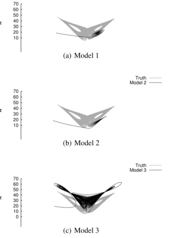
Three imperfect models are created by perturbing the standard parameter values as displayed in Table 1. The perturbed values differ from the standard values by 30– 40% and in each imperfect model parameter values have been increased as well as decreased. With these perturbations the imperfect models behave quite differently from 20

the truth as can be seen in Fig. 2. Both model 1 and 2 are attracted to a point, whereas model 3 has a chaotic solution that resembles the truth, but the attractor is displaced and larger. All models were initiated from the same state and the transient evolution towards the attractor is plotted as well.

By using bifurcation methods, it can be analytically shown that there exists a Hopf 25

(8)

ESDD

1, 247–296, 2010

learning

Title Page

Tables Figures

◭ ◮

Back Close

Full Screen / Esc

Discussion

P

a

per

|

Dis

cussion

P

a

per

|

Discussion

P

a

per

|

Discussio

n

P

a

per

|

bifurcation, whereas model 3 has a value forρthat lies far above the Hopf bifurcation. For the truth the value ofρlies above the Hopf bifurcation as well, which is why model 3 and the truth have similar behaviour.

The minimization procedure outlined above successfully identified a minimum of the cost function with a value of 0.02. By comparison the value of the cost function for an 5

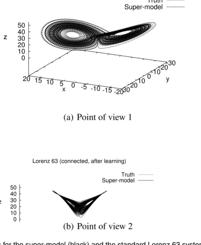
arbitrary choice of all connection coefficients equal to unity is 0.5. With the connection coefficients of this minimum we performed a long integration with the super-model and plotted the trajectory in Fig. 3. The attractor of the super-model is very close to the true attractor. While integrating the super-model, the imperfect models fall into an approximate synchronous behaviour due to the connections: the temporal correlations 10

between thex,y, andzvariables of the three models are in excess of 0.95 (not shown) and the sum of the time-mean distances between the three model states normalized by the sum of the standard deviations ofx_s,y_sandz_sis 0.34. In particular thez-values of the third model are systematically larger than those of the other two models (see Fig. 4). The improvement in the behaviour of the connected imperfect model solutions 15

as depicted in Fig. 4 (to be compared with Fig. 2) is a clear indication of the feasibility of super-modeling in the context of this low-dimensional chaotic system.

In addition to this minimum, we found that by choosing different initial values for the connection coefficients in the minimization procedure different local minima in the cost function are obtained with values of the cost function that are of comparable magnitude. 20

In the remainder of this section we will test the robustness of the learning process, research the issue of local minima and develop measures to determine the quality of the different super-model solutions.

3.1 Robustness

The minimum of the cost function is determined on a limited period of observations 25

of length (K−1)×d_+∆ that we refer to as the training set. We have chosen K₌200 to determine the minimum and subsequently evaluate the cost function using the

(9)

ESDD

1, 247–296, 2010

learning

Title Page

Tables Figures

◭ ◮

Back Close

Full Screen / Esc

Discussion

P

a

per

|

Dis

cussion

P

a

per

|

Discussion

P

a

per

|

Discussio

n

P

a

per

|

K₌20,50,100,150. Cross sections of the cost function around the minimum can be created by changing one connection coefficient and keeping the others fixed at the val-ues of the minimum. The cross sections for the different subsets are plotted in Fig. 5 for connection coefficientsCy₂₃andCz₂₁, since these are typical examples.

In Fig. 5a the cost function forK₌200 displays one well defined minimumCy₂₃₌10.1. 5

The position of the minimum does not change much when the cost function is cal-culated using the different subsets. The minimum becomes more pronounced as the training set is enlarged. The values of the cost function monotonically converge and

K₌200 seems a reasonable size of the training set. Figure 5b does not show a well defined minimum for anyK. Note that the scale is smaller than in Fig. 5a. The values of 10

the cost function do not change much in the different subsets and the slopes are very flat. Changing connection coefficientCz₂₁apparently does not change the quality of the solutions much. A family of super models of similar quality can be found by changing connection coefficientCz₂₁between 8 and 14.

Ideally the super-model found by the learning process is not dependent on the train-15

ing set. To test whether K₌200 is large enough for this to be true the cost function is plotted in Fig. 6 for different periods of observations: the training set and indepen-dent sets of the same size that were obtained from a longer consecutive integration of the truth. Again the cross sections for connection coe_fficientsC₂₃y and C₂₁z are shown (Fig. 6). In Fig. 6a the position and value of the minimum remain close to that of the 20

training set. In Fig. 6b the cost function is flat for all sets of observations. We conclude that withK₌200 the cost function verifies rather well on independent data, soK₌200 seems a reasonable size of the training set.

3.2 Local minima

In the previous section we noted that there is a large family of super-model solutions 25

(10)

ESDD

1, 247–296, 2010

learning

Title Page

Tables Figures

◭ ◮

Back Close

Full Screen / Esc

Discussion

P

a

per

|

Dis

cussion

P

a

per

|

Discussion

P

a

per

|

Discussio

n

P

a

per

|

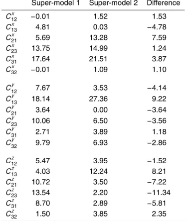
distribution. In this way we found other minima that are distinct in many more connec-tion coe_fficients. For one of these minima, the connection coe_fficients are shown in Table 2, together with the values for the first minimum. In the fourth column the diff er-ence between the connection coefficients of minima 1 and 2 indicates that the minima are clearly distinct and do not belong to the same family of solutions.

5

A plot of the attractor of the second super-model solution in its phase space (not shown) looks almost exactly the same as the plots of the first super-model solution in Figs. 3 and 4. The value of the cost function for the second solution is slightly lower (0.003 instead of 0.02) and is a first indication that the second solution might be better. In the next section we will use various measures to evaluate the quality of these two 10

super-model solutions.

3.3 Quality measures

The cost function is a measure of the quality of the short term behaviour of the super-model in which the initial conditions play a role as is the case in weather predictions. To evaluate the quality of the super-model beyond the range that is influenced by the 15

initial conditions, different measures can be used as in climate simulations.

The most straightforward measures are the different moments of the probability den-sity function of the states in phase space, such as the mean, variance and covariance of the state variables. Since these do not take into account the temporal evolution through phase space, we will also evaluate the ability of the super-model to reproduce 20

the autocorrelation functions of the state variables. As a final measure we will check the ability of the super-model to synchronize with the truth at the end of this section.

Mean, standard deviation and covariance

(11)

ESDD

1, 247–296, 2010

learning

Title Page

Tables Figures

◭ ◮

Back Close

Full Screen / Esc

Discussion

P

a

per

|

Dis

cussion

P

a

per

|

Discussion

P

a

per

|

Discussio

n

P

a

per

|

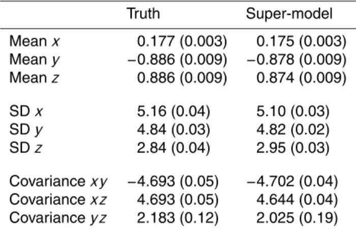
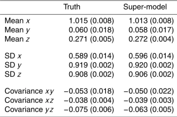
based on the spread of the 500 estimates of each quantity. The results for the imperfect models are given in Table 3 and for the truth and both super-models in Table 4.

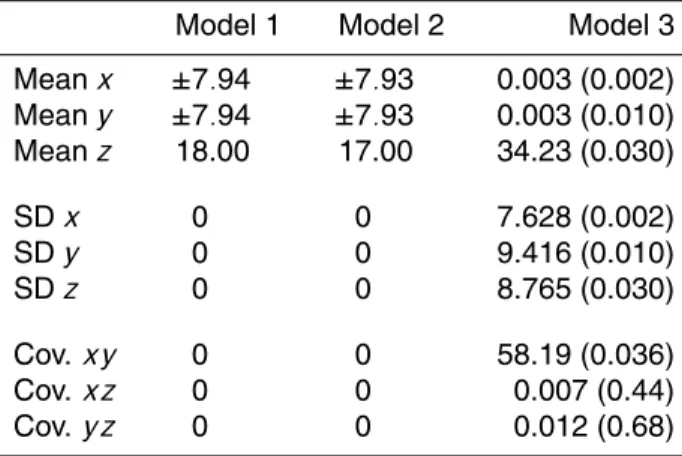
For the parameter values of model 1 and 2 the attractor reduces to two stable point attractors. Thex,y and z values of these fixed points can be calculated analytically from Eq. (1) by setting the time derivatives to zero. Since the system settles in one 5

of these point attractors depending on the initial condition, the mean values are equal to these values. The statistics of the chaotic solution of model 3 (see Table 3) differ substantially from the truth (see Table 4), especially the mean value ofzis much larger. Both super-models (see Table 4) have statistics that are close to that of the truth with the largest differences of order 5% in the covariance between x and y. The second 10

super-model is somewhat closer to the truth, especially in the covariance ofx andy.

3.4 Autocorrelation

The autocorrelation is a statistical measure of the temporal evolution. It gives an in-dication of the memory and time scales present in a system. The plots in Fig. 7 are based on 100 runs of 3000 time units and the shading corresponds to the 95% error 15

range of the autocorrelation of the truth.

Both super-models capture the fast decorrelation ofxandy and the slow decorrela-tion ofzwell, but the second super-model is closer to the truth. It also better represents the dominant time scale which is most apparent in the autocorrelation ofz. After 9 os-cillations super-model 1 is lagging the truth somewhat, whereas super-model 2 is still 20

in phase.

3.5 Synchronization with the truth

Pecora and Carroll (1990) have shown that limited information exchange between two identical Lorenz systems can lead to synchronization of the model states even when the systems are initialized from very di_fferent initial conditions and di_ffer slightly in pa-25

(12)

ESDD

1, 247–296, 2010

learning

Title Page

Tables Figures

◭ ◮

Back Close

Full Screen / Esc

Discussion

P

a

per

|

Dis

cussion

P

a

per

|

Discussion

P

a

per

|

Discussio

n

P

a

per

|

quality of a model. In this section we will compare how well the super-models compare to a perfect model in this respect.

Yang et al. (2006) extended the study of synchronized Lorenz systems, re-interpreted in the context of data assimilation. Following Yang et al. (2006) we add a so-called simple nudging term to the equations of they variable for each of the three connected 5

imperfect models as in Eq. (5). This term “nudges” the actual values of y_k to the observed valuey_oand the value of parameterndetermines the strength of the nudging.

˙

x_k₌σ_k(y_k−x_k)+X

j6=k

Cx_kj(x_j−x_k) (5)

˙

y_k₌x_k(ρ_k−z_k)−y_k₊X

j6=k

C_kjy (y_j−y_k)+n(y_o−y_k)

˙

z_k₌x_ky_k−β_kz_k₊X

j6=k

Cz_kj(z_j−z_k)k₌1,2,3 10

We take the following definition of synchronization:

Definition 1 A model is synchronized with the truth if the RMS difference between the model state and observed true state att₌t₀is smaller thanδand remains smaller than

ǫfort→ ∞.

ǫis chosen larger thanδ, since synchronized systems often deviate somewhat dur-15

ing short extreme excursions of the trajectory, but remain synchronized. As a measure of synchronization we use the minimum strength of the nudgingnfor which synchro-nization is accomplished independent of the initial condition, for integern. For practical purposes we choose a time interval of T₌1000 time units during which the models must remain withinǫdistance of each other.

20

(13)

ESDD

1, 247–296, 2010

learning

Title Page

Tables Figures

◭ ◮

Back Close

Full Screen / Esc

Discussion

P

a

per

|

Dis

cussion

P

a

per

|

Discussion

P

a

per

|

Discussio

n

P

a

per

|

parameter values (what we call the truth) synchronize usingn₌3,δ₌2 andǫ₌4 for all 100 initializations.

To compare the two super-model solutions the same set of 100 initializations are used. The first super-model needs a nudging strength ofn₌11 in order to synchronize with the truth. The second super-model needs a somewhat larger valuen₌13. Using 5

the same experimental setup, we found that the imperfect models individually are not able to synchronize with the truth at all. Both super-models need a stronger nudging than the perfect model. In this measure, the first super-model is closer to the truth, despite the fact that the mean temporal evolution, as measured by the autocorrela-tion, is more faithfully captured by the second super-model that also has a smaller cost 10

function value. However, if we calculate the probability density function of the distance between the truth and the super-model from a 105 time units long integration of the super-model nudged to the truth as in Eq. (5) for n₌6, we find that more often the second super-model remains closer to the truth than the first super-model (see Fig. 8). Nevertheless, the second super-model needs a slightly larger nudging strength to syn-15

chronize with the truth than the first because for nudging values larger thann₌5, it has larger probability, albeit small, of exceeding the thresholdǫ₌4. Forn₌6 the distance between the second super-model and the truth is larger than 4 during 1.6% of the time whereas it is 1.3% for the first. Forn₌10 it is 0.27% for the second and 0.075% for the first. This probability becomes small enough to meet the synchronization criterium of 20

Definition 1 forn₌13 for the second super-model, whereas for the first this happens for

n₌11. We conclude that the interpretation of the ability of a model to synchronize with the truth as a measure of the quality of a solution is not so straightforward.

All measures indicate that the second super-model is closer to the truth than the first. It turns out that the value of the cost function is indeed a good indication of the 25

(14)

ESDD

1, 247–296, 2010

learning

Title Page

Tables Figures

◭ ◮

Back Close

Full Screen / Esc

Discussion

P

a

per

|

Dis

cussion

P

a

per

|

Discussion

P

a

per

|

Discussio

n

P

a

per

|

3.6 Simulating climate change

In order to check whether the super-model is also able to simulate climate change, for instance the response of the truth to a parameter perturbation, we doubled the parameterρ in the true system and in the imperfect models in the super-model. The response of the attractor is an increase in size, the shape remains very similar (see 5

Fig. 9). Although the connection coefficients are learned for ρ₌28, the super-model quite accurately simulates the attractor for ρ₌56. The mean z-value increases with a factor of 2.2 for both the truth as well as the super-model. The response is practically the same for both super-models.

4 Results R ¨ossler and Lorenz 84

10

In this section the super-modeling approach is applied to the R ¨ossler and the Lorenz 84 systems. Both display chaotic behaviour for standard parameter settings, but the at-tractors are quite different.

4.1 R ¨ossler

The Lorenz 63 attractor is also called abutterfly, because of its shape. As a simplifica-15

tion of this example of chaos to one where the attractor only has one “wing”, the R ¨ossler equations were proposed (R ¨ossler, 1976). The time evolution is less chaotic than in the Lorenz 63 system, since it lacks the irregular transitions between two unstable points. The equations are

˙

x₌−(y₊z) 20

˙

y ₌x₊ay (6)

˙

(15)

ESDD

1, 247–296, 2010

learning

Title Page

Tables Figures

◭ ◮

Back Close

Full Screen / Esc

Discussion

P

a

per

|

Dis

cussion

P

a

per

|

Discussion

P

a

per

|

Discussio

n

P

a

per

|

The parameter values for the truth are R ¨osslers values: a₌0.2,b₌0.2 and c₌5.7. The values for the parameters for the three imperfect models can be found in Table 5. The parameter perturbations applied are again of the order 30% to 40% and in each of the imperfect models parameters have been decreased as well as increased.

With these parameter perturbations, marked changes occur in the attractor as can 5

be seen in Fig. 10. The attractor of imperfect model 1 is still chaotic and has a similar shape, but the amplitude of the irregular oscillations is larger. Imperfect model 2 and 3 have a periodic attractor of different shapes.

To determine the super-model we first need to choose values for the different param-eters in the cost function. For the R ¨ossler system the time it takes for initial errors to 10

double is on average 6.7. Following the same procedure as for the Lorenz 63 system we setγ₌0.9 and∆=12 time units. The number of initializations in this case isK₌300. We minimized the cost function by varying the connection coefficients of the super-model. This minimum is plotted in Fig. 11 in a cross section along C₂₃x . The value at the minimum is approximately 0.0001, which is much lower than a typical value 15

of the cost function (0.004 for all connection coefficients equal to 1). To check the robustness of this minimum with respect to the limited size of training set, we calculated the cost function for 9 additional sets of 300 initializations, that were taken from a longer simulation of the truth. The figure shows that 300 initializations are enough to reliably estimate the cost function. This minimum is not unique. By changing the initial values 20

of the connection coefficients in the minimization procedure, we found different minima with similar values of the cost function as was the case for the Lorenz 63 system. Here we evaluate the quality of this minimum only.

With the connection coefficients of this minimum, we integrated the super-model and plotted the trajectory of the three connected imperfect models in Fig. 12. The three 25

(16)

ESDD

1, 247–296, 2010

learning

Title Page

Tables Figures

◭ ◮

Back Close

Full Screen / Esc

Discussion

P

a

per

|

Dis

cussion

P

a

per

|

Discussion

P

a

per

|

Discussio

n

P

a

per

|

three model states normalized by the sum of the standard deviations ofx_s,y_sandz_sis 0.18. The super-model solution, which is defined as the average of the three imperfect models, is plotted in Fig. 13 for two points of view. Visually the attractor of the super model is very similar to the true attractor. We will apply the same measures as for the Lorenz 63 system to check the quality of the super-model.

5

First we compare the means, standard deviations and covariances for the uncon-nected imperfect models in Table 6 and for the super-model and the truth in Table 7. The super-model turns out to be closer to the truth than the best imperfect model (model 3). Its statistics almost fall within the 95% error bounds of the true values.

To compare the temporal behaviour we calculated the autocorrelation functions as 10

plotted in Fig. 14 for the truth and the super-model. They indicate a strongly periodic behaviour with a long decorrelation time scale. For all three variables the autocorrela-tion funcautocorrela-tion is close to and sometimes within the 95% error band, again indicating that the super-model is a very good approximation of the truth.

Finally we look at the minimum nudging strength needed to enable synchronization 15

with the truth. We use the same definition of synchronization as for the Lorenz 63 model with the following values for the parameters δ₌0.05, ǫ₌0.4 and T₌1000 time units. When the nudging term is applied to theyvariable only, we find that the standard R ¨ossler system synchronizes with a copy of itself for a nudging strength equal ton₌1. The super-model also synchronizes when nudging only the y variable, but it needs 20

a stronger nudging ofn₌2. It outperforms model 3 in this measure; even by replacing they variable with the true value (which corresponds effectively to an infinitely large nudging strength), synchronization does not occur.

To conclude, also in the case of the R ¨ossler system, super-model solutions can be found by combining imperfect models that give a very good approximation to the truth. 25

(17)

ESDD

1, 247–296, 2010

learning

Title Page

Tables Figures

◭ ◮

Back Close

Full Screen / Esc

Discussion

P

a

per

|

Dis

cussion

P

a

per

|

Discussion

P

a

per

|

Discussio

n

P

a

per

|

more degrees of freedom to mimick the truth. Beforehand it is hard to predict whether more chaos helps or hurts, so we test the super-modeling approach also on the more chaotic Lorenz 84 system.

4.2 Lorenz 84

The Lorenz 84 system was proposed by Lorenz as a toy model for the general atmo-5

spheric circulation at midlatitudes (Lorenz, 1984). The model equations are

˙

x₌−y2−z2−ax₊aF

˙

y ₌xy−bxz−y₊G (7)

˙

z₌bxy₊xz−z.

Thex variable represents the intensity of the globe-encircling westerly winds andy

10

andz represent a travelling large-scale wave that interacts with the westerly wind. Pa-rametersF andGare forcing terms representing the average north-south temperature contrast and the east-west asymmetries due to the land-sea distribution, respectively.

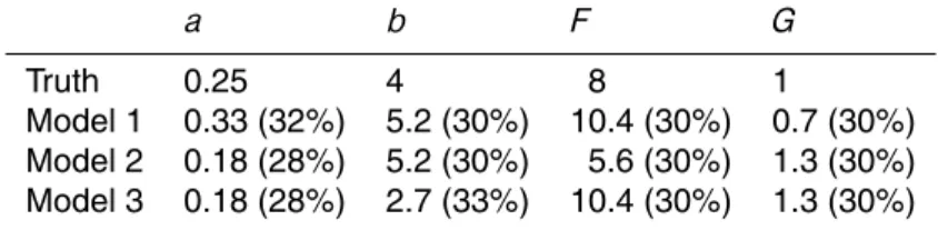
The standard parameter values for the truth area₌1₄,b₌4,F₌8 andG₌1, for which the model displays chaotic behaviour (van Veen, 2001). In Table 8 the perturbed pa-15

rameter values of the imperfect models are given. The perturbations are again about 30% and in each imperfect model parameters have been decreased as well as in-creased.

With these parameter perturbations the attractor of the imperfect models differ sub-stantially from the truth (see Fig. 15). Both model 1 and 3 have periodic attractors, 20

whereas model 2 has a point attractor (the transient evolution towards the point attrac-tor is shown for model 2). The periodic behaviour corresponds to the wave traveling periodically around the hemisphere.

(18)

ESDD

1, 247–296, 2010

learning

Title Page

Tables Figures

◭ ◮

Back Close

Full Screen / Esc

Discussion

P

a

per

|

Dis

cussion

P

a

per

|

Discussion

P

a

per

|

Discussio

n

P

a

per

|

for initial errors to double (on average 1.1 time units). However with these values the minimization algorithm did not produce a well defined minimum of the cost function. The high value of the autocorrelation function ofx (0.6 at 8 time units, see Fig. 18) indicates that the initial conditions still have an impact on the evolution after 8 time units. Therefore we decided to increase _∆ to 8 and γ to 0.8. In addition it turned 5

out that it was easier to find good minima using the amoeba minimization algorithm (Nelder and Mead, 1965) instead of the conjugate gradients minimization. The amoeba method does not need gradient information and is less susceptible to getting stuck in local minima. The training set is based onK₌200 initializations, each 0.2 time units apart selected from a long simulation of the truth.

10

Starting from di_fferent initial values for the connection coe_fficients we found di_fferent minima of the cost function. A cross section through the best minimum that we found is shown in Fig. 16. The value at this minimum is approximately 0.0003, which is again much lower than the value of the costfunction for all connection coe_fficients equal to 1 (0.08). To check the robustness the cost function is evaluated on 9 additional 15

independent sets of 200 initializations. In all 9 sets the minimum is reproduced around the same value of the connection coefficient. The same is true for cross sections of the other connection coefficients (not shown).

With the connection coefficients for this minimum, we integrated the super-model and plotted the trajectory in Fig. 17. A visual comparison with the truth indicates a very good 20

agreement. In this case the three imperfect models are almost perfectly synchronized (not shown). The synchronization is stronger in this case as compared to the other two systems. The temporal correlations between thex,y andz variables of the three imperfect models in the super-model are in excess of 0.99 and the sum of the time-mean distances between the three model states normalized by the sum of the standard 25

(19)

ESDD

1, 247–296, 2010

learning

Title Page

Tables Figures

◭ ◮

Back Close

Full Screen / Esc

Discussion

P

a

per

|

Dis

cussion

P

a

per

|

Discussion

P

a

per

|

Discussio

n

P

a

per

|

solutions closer together. Maximum values of the connection coefficients in the other two systems are a factor of 10 smaller.

Again we use the same measures to evaluate the quality of the super-model solution. The mean, standard deviation and covariance for the truth and the super-model are presented in Table 9. These statistics are in excellent agreement.

5

In order to evaluate the temporal behaviour we compare the autocorrelation functions in Fig. 18. Up to a delay time of 14 time units the autocorrelation functions of the truth are well reproduced by the super model both in shape as well as in periodicity.

The Lorenz 84 system with standard parameter values synchronizes with the truth for a strength of the nudging termn₌1 in they variable only, usingδ₌0.1,ǫ₌0.5 and 10

T₌1000 in Definition 1. The super-model also synchronizes with the truth, but it needs a larger nudging ofn₌4. None of the imperfect models is able to synchronize with the truth, when the nudging is in they variable only.

Concluding this section, super-model solutions can be found that reproduce the true system very well and outperform the individual imperfect models for the Lorenz 84 sys-15

tem as well. For this system, the minimization process was found to be more sensitive to the length of the short integrations ∆ and the discount parameter γ, requiring the use of the more robust amoeba minimization procedure.

5 Conclusion and discussion

In this study we developed and tested a novel multi model ensemble approach in which 20

imperfect models of an observable system are combined into a single super-model by letting the models exchange information during the simulation. The information exchange takes the form of linear connections with weights that are learned from past data such that the super-model minimizes the mean squared errors in short simulations initialized from past observed states. The main result of this study is that it is possible 25

(20)

ESDD

1, 247–296, 2010

learning

Title Page

Tables Figures

◭ ◮

Back Close

Full Screen / Esc

Discussion

P

a

per

|

Dis

cussion

P

a

per

|

Discussion

P

a

per

|

Discussio

n

P

a

per

|

This result motivates an alternative strategy to the weather and climate prediction problem. Current practice is that existing imperfect models of the climate system are integrated independently of one another, starting from observed initial conditions to provide forecasts for the future. To gauge model uncertainty, the outcomes of the different models are combined into a single estimate of the probability density function 5

of climate variables. This study indicates that better estimates of the true probability function can be obtained if the models are taught, using past observations, to combine the strengths of each into a single forecast of the probability density function.

A large gap exists between the simple, chaotic systems of this study and the com-plex, state-of-the-art climate models. Many questions need to be addressed in order to 10

apply the same approach to these models. There is the practical limitation of computer capacity to enable the parallel execution of an ensemble of state-of-the-art models that need to exchange information at every time step. In the study of Kirtman et al. (2003) two atmospheric models were coupled to one ocean model so in principle it should be feasible to couple several atmospheric models to several ocean models. Compu-15

tational grids in the various climate models differ, so regridding should be part of the information exchange. Regridding is standard practice in the information exchange be-tween the atmosphere and ocean components of climate models. An important issue is the choice of state variables for the connections and the number of connections. In this study all state variables were connected and had similar dynamics. In the climate 20

models the di_fferent state variables are driven by di_fferent physical processes and dis-play distinct dynamical behaviour at various time scales. It is not clear a priori which state variables should be connected. In addition the number of connections that can be learned on the basis of historical data is limited and therefore careful choices for the connections need to be made. One possible approach would be to not connect 25

(21)

ESDD

1, 247–296, 2010

learning

Title Page

Tables Figures

◭ ◮

Back Close

Full Screen / Esc

Discussion

P

a

per

|

Dis

cussion

P

a

per

|

Discussion

P

a

per

|

Discussio

n

P

a

per

|

A hierarchy of earth system models of intermediate complexity (EMICs) could be used to address these various issues. The EMIC’s resemble the state-of-the-art cli-mate models in their structure, but differ in that the parameterization schemes for the physical processes are much less elaborate, fewer processes are explicitly modeled and the spatial resolution is much coarser. It has already been demonstrated that 5

two different quasi-geostrophic channel models will synchronize with only limited con-nections (Duane and Tribbia, 2001, 2004). A fruitful strategy might be to start from a relatively simple climate model and add to the complexity in small steps and ad-dress a specific issue at each step. In a similar fashion as in this study a ground truth model is assumed at each time step and an ensemble of imperfect models is created 10

by perturbing parameters and/or using di_fferent formulations for unresolved processes. An additional complicating factor for the learning phase is the difference in time-scale between atmosphere and ocean. Adjustments in the atmosphere have a short time scale, but the ocean adapts to these changes on a much longer time-scale. Through its influence on the atmosphere, the ocean introduces longer time scales in the atmo-15

sphere as well. So short integrations during the learning phase do not probe these e_ffects. This might hamper the learning. On the other hand, there are indications that fast atmospheric processes are the primary cause of model systematic errors (Rodwell and Jung, 2008).

An alternative learning strategy that is explicitly based on synchronization is outlined 20

in the study by Duane et al. (2007). In this strategy the super-model equations con-tain nudging terms to the truth as in our Eq. (5) and additional evolution equations are formulated for the parameters. If the super-model synchronizes with the truth the pa-rameters stop updating. This alternative learning strategy leads to a particularly simple learning law that would be useful in the implementation of the super-model approach 25

using more complex models. The strategy has been demonstrated with Lorenz sys-tems (Duane et al., 2009).

(22)

ESDD

1, 247–296, 2010

learning

Title Page

Tables Figures

◭ ◮

Back Close

Full Screen / Esc

Discussion

P

a

per

|

Dis

cussion

P

a

per

|

Discussion

P

a

per

|

Discussio

n

P

a

per

|

problem and makes finding a suitable super-model solution easier. The existence of quite distinct super-model solutions of good quality remains a bit of a mystery.

The main caveat is that the super-model is trained on historical data and in a climate prediction problem is subsequently applied to simulate the response of the system to an external forcing. It is therefore not guaranteed that the super-model will also simu-5

late this response more realistically. The problem is not peculiar to the super-modeling approach, but arises with climate models generally, since they are “tuned” on historical data and are used to predict the climate response to a change in greenhouse gas con-centrations. In this study we obtained the encouraging result that for the Lorenz 1963 system the super-model was able to accurately predict the change to a doubling of the 10

parameterρ. In the super-modeling approach this issue can be further addressed in a similar perfect model setting using climate models of increasing complexity.

References

Compo, G., Whitaker, J., and Sardeshmukh, P.: Feasibility of a 100-year reanalysis using only surface pressure data, B. Am. Meteor. Soc., 87, 175–189, 2006. 249

15

Duane, G. and Tribbia, J.: Synchronized chaos in geophysical fluid dynamics, Phys. Rev. Lett., 86, 4298–4301, 2001. 267

Duane, G. and Tribbia, J.: Weak Atlantic-Pacific teleconnections as synchronized chaos, J. At-mos. Sci., 61, 2149–2168, 2004. 267

Duane, G. S., Tribbia, J. J., and Weiss, J. B.: Synchronicity in predictive modelling: a new view

20

of data assimilation, Nonlin. Processes Geophys., 13, 601–612, doi:10.5194/npg-13-601-2006, 2006. 249

Duane, G., Yu, D., and Kocarev, L.: Identical synchronization, with translation invariance, im-plies parameter estimation, Phys. Lett. A, 371, 416–420, 2007. 267

Duane, G., Tribbia, J., and Kirtman, B.: Consensus on Long-Range Prediction by Adaptive

25

Synchronization of Models, EGU General Assembly, Vienna, Austria, 2009. 267

(23)

ESDD

1, 247–296, 2010

learning

Title Page

Tables Figures

◭ ◮

Back Close

Full Screen / Esc

Discussion

P

a

per

|

Dis

cussion

P

a

per

|

Discussion

P

a

per

|

Discussio

n

P

a

per

|

IPCC: Climate Change 2007: The Physical Science Basis, Contribution of Working Group I to the Fourth Assessment Report of the Intergovernmental Panel on Climate Change, edited by: Solomon, S., Qin, D., Manning, M., Chen, Z., Marquis, M., Averyt, K. B., Tignor, M., and Miller, H. L., Cambridge University Press, Cambridge, UK and New York, USA, 2007. 248 Kirtman, B., Min, D., Schopf, P., and Schneider, E.: A new approach for CGCM sensitivity

5

studies, COLA Technical Report, 154, 50 pp., 2003. 249, 266

Lorenz, E.: Deterministic nonperiodic flow, J. Atmos. Sci., 20, 130–140, 1963. 250

Lorenz, E.: Irregularity, a fundamental property of the atmosphere, Tellus A, 36, 98–110, 1984. 263

Nelder, J. and Mead, R.: A simplex method for function minimization, Comp. J., 7, 308–313,

10

1965. 264

Pecora, L. and Carroll, T.: Synchronization in chaotic systems, Phys. Rev. Lett., 64, 824–824, 1990. 249, 257

Rodwell, M. and Jung, T.: Understanding the local and global impacts of model physics changes: an aerosol example, Q. J. Roy. Meteor. Soc., 134, 1479–1497, 2008. 267

15

R ¨ossler, O.: An equation for continuous chaos, Phys. Lett., 75A, 397–398, 1976. 260

Tebaldi, C. and Knutti, R.: The use of the multi-model ensemble in probabilistic climate projec-tions, Philos. T. Roy. Soc. A, 365, 2053–2075, 2007. 249

van Veen, L.: Active and passive ocean regimes in a low-order climate model, Tellus A, 53, 616–628, 2001. 263

20

(24)

ESDD

1, 247–296, 2010

learning

Title Page

Tables Figures

◭ ◮

Back Close

Full Screen / Esc

Discussion

P

a

per

|

Dis

cussion

P

a

per

|

Discussion

P

a

per

|

Discussio

n

P

a

per

|

Table 1.Standard and perturbed parameters for the Lorenz 63 system.

σ ρ β

Truth 10 28 8

3

(25)

ESDD

1, 247–296, 2010

learning

Title Page

Tables Figures

◭ ◮

Back Close

Full Screen / Esc

Discussion

P

a

per

|

Dis

cussion

P

a

per

|

Discussion

P

a

per

|

Discussio

n

P

a

per

|

Table 2.The connection coefficients of two super-model solutions of the Lorenz 63 system and their differences.

Super-model 1 Super-model 2 Difference

C₁₂x −0.01 1.52 1.53

C₁₃x 4.81 0.03 −4.78

C₂₁x 5.69 13.28 7.59

C₂₃x 13.75 14.99 1.24

C₃₁x 17.64 21.51 3.87

C₃₂x −0.01 1.09 1.10

C₁₂y 7.67 3.53 −4.14

C₁₃y 18.14 27.36 9.22

C₂₁y 3.64 0.00 −3.64

C₂₃y 10.06 6.50 −3.56

C₃₁y 2.71 3.89 1.18

C₃₂y 9.79 6.93 −2.86

C₁₂z 5.47 3.95 −1.52

C₁₃z 4.03 12.24 8.21

C₂₁z 10.72 3.50 −7.22

C₂₃z 13.54 2.20 −11.34

C₃₁z 8.70 2.89 −5.81

(26)

ESDD

1, 247–296, 2010

learning

Title Page

Tables Figures

◭ ◮

Back Close

Full Screen / Esc

Discussion

P

a

per

|

Dis

cussion

P

a

per

|

Discussion

P

a

per

|

Discussio

n

P

a

per

|

Table 3. Mean, standard deviation (SD) and covariance for the three unconnected imperfect models of the Lorenz 63 system. The values for the first two models are calculated analytically. Statistics for model 3 are based on 500 runs of 5000 time units. Between brackets the 95% error estimation is given.

Model 1 Model 2 Model 3

Meanx ±7.94 ±7.93 0.003 (0.002) Meany ±7.94 ±7.93 0.003 (0.010) Meanz 18.00 17.00 34.23 (0.030)

SDx 0 0 7.628 (0.002)

SDy 0 0 9.416 (0.010)

SDz 0 0 8.765 (0.030)

Cov.xy 0 0 58.19 (0.036)

Cov.xz 0 0 0.007 (0.44)

(27)

ESDD

1, 247–296, 2010

learning

Title Page

Tables Figures

◭ ◮

Back Close

Full Screen / Esc

Discussion

P

a

per

|

Dis

cussion

P

a

per

|

Discussion

P

a

per

|

Discussio

n

P

a

per

|

Table 4. Mean, standard deviation (SD) and covariance for the truth and for the two super-models of the Lorenz 63 system. Statistics are based on 500 runs of 5000 time units. Between brackets the 95% error estimation is given.

(28)

ESDD

1, 247–296, 2010

learning

Title Page

Tables Figures

◭ ◮

Back Close

Full Screen / Esc

Discussion

P

a

per

|

Dis

cussion

P

a

per

|

Discussion

P

a

per

|

Discussio

n

P

a

per

|

Table 5.Standard and perturbed parameters for the R ¨ossler system.

a b c

Truth 0.2 0.2 5.7

(29)

ESDD

1, 247–296, 2010

learning

Title Page

Tables Figures

◭ ◮

Back Close

Full Screen / Esc

Discussion

P

a

per

|

Dis

cussion

P

a

per

|

Discussion

P

a

per

|

Discussio

n

P

a

per

|

Table 6. Mean, standard deviation (SD) and covariance for the three unconnected imperfect models of the R ¨ossler system. The 95% error estimation based on 500 runs of 5000 time units is given between brackets.

Model 1 Model 2 Model 3

(30)

ESDD

1, 247–296, 2010

learning

Title Page

Tables Figures

◭ ◮

Back Close

Full Screen / Esc

Discussion

P

a

per

|

Dis

cussion

P

a

per

|

Discussion

P

a

per

|

Discussio

n

P

a

per

|

Table 7. Mean, standard deviation (SD) and covariance for the truth and super-model of the R ¨ossler system. The 95% error estimation based on 500 runs of 5000 time units is given between brackets.

Truth Super-model

Meanx 0.177 (0.003) 0.175 (0.003) Meany −0.886 (0.009) −0.878 (0.009) Meanz 0.886 (0.009) 0.874 (0.009)

SDx 5.16 (0.04) 5.10 (0.03)

SDy 4.84 (0.03) 4.82 (0.02)

SDz 2.84 (0.04) 2.95 (0.03)

(31)

ESDD

1, 247–296, 2010

learning

Title Page

Tables Figures

◭ ◮

Back Close

Full Screen / Esc

Discussion

P

a

per

|

Dis

cussion

P

a

per

|

Discussion

P

a

per

|

Discussio

n

P

a

per

|

Table 8.Standard and perturbed parameters for the Lorenz 84 system.

a b F G

Truth 0.25 4 8 1

(32)

ESDD

1, 247–296, 2010

learning

Title Page

Tables Figures

◭ ◮

Back Close

Full Screen / Esc

Discussion

P

a

per

|

Dis

cussion

P

a

per

|

Discussion

P

a

per

|

Discussio

n

P

a

per

|

Table 9.Mean, standard deviation (SD) and covariance for the super-model and the standard Lorenz 84 system. The 95% error estimation based on 500 runs of 5000 time units is given between brackets.

Truth Super-model

(33)

ESDD

1, 247–296, 2010

learning

Title Page

Tables Figures

◭ ◮

Back Close

Full Screen / Esc

Discussion

P

a

per

|

Dis

cussion

P

a

per

|

Discussion

P

a

per

|

Discussio

n

P

a

per

|

(34)

ESDD

1, 247–296, 2010

learning

Title Page

Tables Figures

◭ ◮

Back Close

Full Screen / Esc

Discussion

P

a

per

|

Dis

cussion

P

a

per

|

Discussion

P

a

per

|

Discussio

n

P

a

per

|

10 20 30 40 50 60 70

z

Truth Model 1

z

(a) Model 1

10 20 30 40 50 60 70

z

Truth Model 2

z

(b) Model 2

0 10 20 30 40 50 60 70

z

Truth Model 3

z

(c) Model 3

(35)

ESDD

1, 247–296, 2010

learning

Title Page

Tables Figures

◭ ◮

Back Close

Full Screen / Esc

Discussion

P

a

per

|

Dis

cussion

P

a

per

|

Discussion

P

a

per

|

Discussio

n

P

a

per

|

-20 -15 -10 -5 0 5 10 15 20

-30 -20 -10 0 10 20 30 0

10 20 30 40 50

z

Lorenz 63 (connected, after learning)

Truth Super-model

x

y z

(a) Point of view 1

0 10 20 30 40 50 z

Lorenz 63 (connected, after learning) Truth Super-model

z

(b) Point of view 2

(36)

ESDD

1, 247–296, 2010

learning

Title Page

Tables Figures

◭ ◮

Back Close

Full Screen / Esc

Discussion

P

a

per

|

Dis

cussion

P

a

per

|

Discussion

P

a

per

|

Discussio

n

P

a

per

|

0 10 20 30 40 50 60

z

Lorenz 63 (model 1, connected, after learning)

Truth Model 1

z

(a) Model 1

0 10 20 30 40 50 60

z

Truth Model 2

z

(b) Model 2

0 10 20 30 40 50 60

z

Truth Model 3

z

(c) Model 3