Concentration Dynamics
Geir Halnes1*, Ivar Østby1, Klas H. Pettersen2, Stig W. Omholt3, Gaute T. Einevoll1
1Department of Mathematical Sciences and Technology, Norwegian University of Life Sciences, A˚s, Norway, 2Centre for Integrative Genetics, Department of Mathematical Sciences and Technology, Norwegian University of Life Sciences, A˚s, Norway,3Centre for Integrative Genetics, Department of Animal and Aqucultural Sciences, Norwegian University of Life Sciences, A˚s, Norway
Abstract
The cable equation is a proper framework for modeling electrical neural signalling that takes place at a timescale at which the ionic concentrations vary little. However, in neural tissue there are also key dynamic processes that occur at longer timescales. For example, endured periods of intense neural signaling may cause the local extracellular K+-concentration to increase by several millimolars. The clearance of this excess K+depends partly on diffusion in the extracellular space, partly on local uptake by astrocytes, and partly on intracellular transport (spatial buffering) within astrocytes. These processes, that take place at the time scale of seconds, demand a mathematical description able to account for the spatiotemporal variations in ion concentrations as well as the subsequent effects of these variations on the membrane potential. Here, we present a general electrodiffusive formalism for modeling of ion concentration dynamics in a one-dimensional geometry, including both the intra- and extracellular domains. Based on the Nernst-Planck equations, this formalism ensures that the membrane potential and ion concentrations are in consistency, it ensures global particle/charge conservation and it accounts for diffusion and concentration dependent variations in resistivity. We apply the formalism to a model of astrocytes exchanging ions with the extracellular space. The simulations show that K+-removal from high-concentration regions is driven by a local depolarization of the astrocyte membrane, which concertedly (i) increases the local astrocytic uptake of K+, (ii) suppresses extracellular transport of K+, (iii) increases axial transport of K+ within astrocytes, and (iv) facilitates astrocytic relase of K+in regions where the extracellular concentration is low. Together, these mechanisms seem to provide a robust regulatory scheme for shielding the extracellular space from excess K+.
Citation:Halnes G, Østby I, Pettersen KH, Omholt SW, Einevoll GT (2013) Electrodiffusive Model for Astrocytic and Neuronal Ion Concentration Dynamics. PLoS Comput Biol 9(12): e1003386. doi:10.1371/journal.pcbi.1003386
Editor:Olaf Sporns, Indiana University, United States of America
ReceivedApril 24, 2013;AcceptedOctober 24, 2013;PublishedDecember 19, 2013
Copyright:ß2013 Halnes et al. This is an open-access article distributed under the terms of the Creative Commons Attribution License, which permits unrestricted use, distribution, and reproduction in any medium, provided the original author and source are credited.
Funding:The project was supported by the Research Council of Norway (eVITA program; project numbers 178892 and 178901 and ISP-Fysikk; project number 216699), and EU Grant 269921 (BrainScaleS). The funders had no role in study design, data collection and analysis, decision to publish, or preparation of the manuscript.
Competing Interests:The authors have declared that no competing interests exist. * E-mail: [email protected]
Introduction
The interaction between neurons and glial cells has been the topic of many recent studies within the field of neuroscience (see reviews in [1–3]). Astrocytes (a species of glial cells) play an important role in modulating excitatory and inhibitory synapses by removal, metabolism, and release of neurotransmitters [4], homeostatic maintenance of extracellular K+, H+, and glutamate [5], supply of energy substrates for neurons [6], and neuronal pathfinding during development and regeneration [7]. Astrocytic cells seem to have key roles in many central nervous system disorders, ranging from neuropathic pain and epilepsy to neurodegenerative diseases such as Alzheimers, schizophrenia and depression [8]. Computational models of neuron-glia inter-actions is a prerequisite for understanding the dysfunctional situations, and for assessing glial cells as a potential therapeutic target [9]. To give a few examples, such models have been used to simulate glial regulation of extracellular K+-concentration [10– 13], and the relation between extracellular K+-dynamics and epileptic seizures [14–16] and spreading depression [17,18].
Regulation of the extracellular K+-concentration is considered one of the key cellular functions of astrocytes [2]. During normal
conditions, the extracellular K+-concentration (½Kz
E) is typically maintained close to the baseline level (*3 mM). However, when neurons fire action potentials, they expel K+into the extracellular space. During periods of intense neural activity, the local extracellular K+-concentration may increase by several millimo-lars, and may interfere with neural activity [10,19,20]. Concen-trations between 8 and 12 mM are often considered a limit to pathological conditions [3,12,21].
Orkand (1966) [22] discovered that astrocytes can funnel out excess K+from high concentration regions by a process coined spatial buffering [12,21,22]. According to this concept, K+is taken up by the glial cell from high-concentration sites, evoking a local depolarization of the glial membrane. K+ is then transported longitudinally inside the glial cell (and possibly through several glial cells connected by gap junctions into a glial syncytium [10,23]), and eventually expelled into the ECS at more distal cites where½Kz
Eis lower. However, it has also been argued that astrocytes may reduce ½Kz
Electrical neural signalling is typically modeled using the cable equation, where dendrites and axons are represented as one-dimensional, possibly branching, electrical cables, and the transmembrane potential is the key dynamical variable [26,27]. With the possible exception of the signalling molecule Ca2+(see e.g., [28,29]), ion concentrations are typically assumed to be constant. The effect of ionic diffusion (due to concentration gradients) on the net electrical currents is neglected in standard cable theory, and resistivities (which in reality depend on ion concentrations) are assumed to be constant. These are often good approximations, as concentrations of the main charge carriers (K+, Na+ and Cl2) in the extracellular- (ECS) or intracellular space
(ICS) typically vary little at the short time-scale relevant for electrical neural activity (v100 ms).
Glial function typically involves processes that take place at a longer time-scale (w1 s), at which significant variations in ionic concentrations may occur. For example, the process of spatial K+ -buffering involves local uptake, a local depolarization of the astrocytic membrane, and longitudinal electrodiffusive transports through the intracellular- (ICS) and extracellular space (ECS) propelled both by voltage- and concentration gradients [30]. A mechanistic understanding of glial function thus requires a modelling scheme that in a consistent way can capture the intricate interplay between ion concentration dynamics and the dynamics ofvM. Physically,vMis determined by the total electrical charge on the inside (or outside) of the membrane, which in turn is uniquely determined by the concentrations (½k) of all ionic species that are present there [31]. In some heart cell models, ion concentrations have been reported to drift to unrealistic values in long-term simulations, whilevMmaintain realistic values [32–34]. Whether the relationship betweenvM and ½kis consistent, is a general concern with models that explicitly depend on both. If applied to general problems, and in particular in long-term simulations, models that do not ensure an internally consistent ½k{vM relationship may give erroneous predictions.
Gardner-Medwin (1983) [10] proposed a pioneering computa-tional model of the spatial buffering process, later re-analyzed by Chen and Nicholson (2000) [12]. In this model, spatial buffering
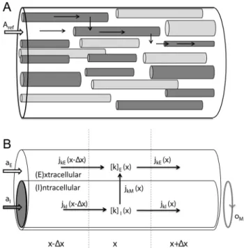
was considered as an essentially one-dimensional transport process. The complex composition of the tissue (Fig. 1A) could then be simplified to a two-domain model as that illustrated in Fig. 1B[10,12]. There, the ICS of all cells participating in the transport process (i.e. the astrocytes) have been represented as an equivalent cable (I-domain) which is coated by ECS (E-domain). The I-E system could be pictured phenomenologically as an representative single astrocyte, coated with the average proportion of available ECS per astrocyte. This geometrical simplification was motivated for one-dimensional transport phenomena through the glial syncytium [10,12], but could in principle apply to any transport phenomena that justifies a geometrical simplification as that in Fig. 1. A limitation with these modelling studies [10,12], and related modelling studies by Newman and coworkers [11,21], is thatvM was derived from standard cable theory, which neglects effect from diffusive currents on vM. The concern regarding a consistent relationship betweenvM and the ionic concentrations thus also applies to these models.
Qian and Sejnowski (1989) have previously developed a consistent, electrodiffusive scheme for modelling the dynamics onvMand ion concentrations [31]. Like the standard cable model, the electrodiffusive model assumes that transport phenomena are essentially one-dimensional. Unlike the standard cable model, the
Figure 1. A two domain-model for ion concentration dynamics in the intra- and extracellular space, when macroscopic transport is essentially one-dimensional.(A) A piece of neural tissue with cross section areaArefand an arbitrary extensionlin thex -direction. The tissue contains cells (dark grey) that participate in the transport process, and cells that do not (light grey). (B) The interior of all participatory cells represented as a single, equivalent cylindrical cable (I), coated by ECS (E). The geometry is specified by three parameters, whereaIandaEare, respectively, the fractions ofAref occupied by the ICS of participatory cells and the ECS, andOM(m{1)is the amount of membrane area per tissue volume (or, equivalently, the circumference of the equivalent cable divided byAref). Due to the presence of other cells (non-participatory), we generally have that aIzaEv1. The concentration of ion species k is denoted ½kn where n represents domainIorE. Ionic movement is described by the transmembrane flux density (jkM) and the longitudinal flux densities due to electrical migration (jknf) and diffusion (jd
kn). doi:10.1371/journal.pcbi.1003386.g001
Author Summary
electrodiffusive model derived vM from the ion concentration dynamics, accounting for all ionic movements (membrane fluxes, longitudinal diffusion, and longitudinal electrical migration), as well as for the concentration-dependent variation of the intracel-lular resistivities. An important limitation with this previous electrodiffusive model is that it only includes intracellular dynamics, whereas the ECS was assumed to be isopotential and with constant ion concentrations [31]. This was a useful simplification for simulating a small intracellular compartment, such as a dendritic spine [31], but is not generally applicable to macroscopic transport mechanisms. In particular, it can not be applied for modelling the spatial buffering process, where ion concentration dynamics in the ECS plays a paramount role. In reality, the ECS comprises about 20% of the total neural tissue volume, while the remaining 80% is the ICS of various cells [12]. When a large number of cells participate in simultaneous ion exchange with the ECS, the impact on the ion concentrations in the ICS and ECS may be of the same order of magnitude.
The aim of this work is twofold: First, we generalize the electrodiffusive formalim [31] to a explicitly include the ECS. The result is a general mathematical framework for consistently modelling the dynamics of the membrane potential (vM), the intra-(½kI) and extracellular (½kE) ion concentrations for a set (k) of ionic species. We believe that this framework will be of general value for the field of neuroscience, as it can be applied to any system that justifies a geometrical description as that in Fig. 1B. Next, we apply the electrodiffusive formalism in a spatially explicit model of astrocytes exchanging ions with the ECS. We run simulations to investigate the efficiency of the spatial K+-buffering process, relative to that of local uptake/storage by astrocytes, and that of diffusion in the ECS alone. Unlike the previous models [10–12,21], our astrocyte model is based on the prevailing view that Na+/K+/ATPase-pump is
the main uptake mechanism for K+[3]. Furthermore, as our model was based on a physically consistent electrodiffusive formalism, we arrive at a full mechanistic description of the buffering process, which quantitatively describes the intricate interplay betweenvM and the dynamics of ion concentrations.
This article is organized in the following way: The Model section contains two main parts. In the first part, we present the electrodiffusive formalism for computing the ion concentration dynamics in a system described by the geometry depicted in Fig. 1B. We consider this theoretical framework a key contribution of this work. However, the key concepts introduced in this part are summarized in Table 1, and with this in hand, the reader who is mainly interested the biological process of spatial K+-buffering by astrocytes may therefore skip to second part of the Model-section. There, the model for astrocytes exchanging ions with the ECS is presented. The Results section is devoted to simulations on the astrocyte model, and provides an improved biophysical insight in the electrodiffusive mechanisms utilized by astrocytes to spatially buffer K+. By comparing different versions of the model, we also assessed the importance of spatial buffering, relative to that of other clearance mechanisms such as local uptake/storage by astrocytes and diffusion through the ECS alone. Finally, in the Discussion section we address how our mathematical framework relates to previous electrodiffusive modeling frameworks. We also summarize the new insights that our simulations have given in the process of spatial K+-buffering by astrocytes.
Model
Electrodiffusive formalism
In Fig. 1B, particles inIor E may move along the x-axis or across the membrane. In a segmentDx ofI, centered atx, and
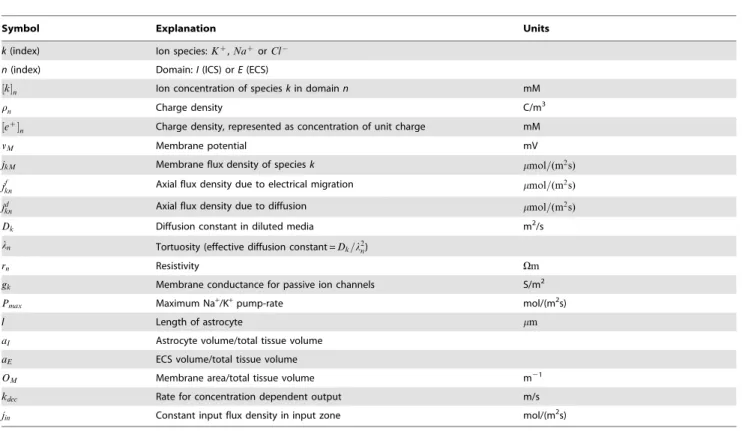
Table 1.List of symbols and definitions.
Symbol Explanation Units
k(index) Ion species:Kz,
Nazor
Cl{
n(index) Domain:I(ICS) orE(ECS)
½kn Ion concentration of specieskin domainn mM
rn Charge density C/m3
½ez
n Charge density, represented as concentration of unit charge mM
vM Membrane potential mV
jkM Membrane flux density of speciesk mmol=(m2s)
jfkn Axial flux density due to electrical migration mmol=(m2s)
jd
kn Axial flux density due to diffusion mmol=(m2s)
Dk Diffusion constant in diluted media m2/s
ln Tortuosity (effective diffusion constant =Dk=l2n)
rn Resistivity Vm
gk Membrane conductance for passive ion channels S/m2
Pmax Maximum Na+/K+pump-rate mol/(m2s)
l Length of astrocyte mm
aI Astrocyte volume/total tissue volume
aE ECS volume/total tissue volume
OM Membrane area/total tissue volume m21
kdec Rate for concentration dependent output m/s
jin Constant input flux density in input zone mol/(m2s)
with volumeaIDx, the particle concentration dynamics of an ion specieskis determined by:
{OMDxjkM(x,t)zaIjkI(x{Dx=2,t)){
aIjkI(xzDx=2,t)~aIDx
L½kI(x,t)
Lt ,
ð1Þ
where the transmembrane- (jkM), the intracellular- (jkI) and the extracellular (jkE) flux densities of particle species k, have units mol/(m2s). The first term on the left represents the ionic flux that enter this segment through the piece of the membrane with area OMDx. The negative sign follows fromjkM (by convention) being defined as positive in the direction fromItoE. The second and third terms represent the ionic fluxes that enter(+)/leave(2) the section through the left/right boundaries, with cross section areas aI. If the net flux into the segment is nonzero, the ion concentration will build up over time, according to the right hand side of Eq. 1.
We divide Eq. 1 byaIDx, and take the limitDx?0, to obtain
the continuity equation on differential form:
LjkI(x,t) Lx z
OM aI
jkM(x,t)z
L½kI(x,t)
Lt ~0 ð2Þ
LjkE(x,t) Lx {
OM aE
jkM(x,t)z
L½kE(x,t)
Lt ~0: ð3Þ
We have also written up the continuity equation for the extracellular domain.
The axial flux densities are described by the generalized Nernst-Planck equation:
jkn(x,t)~{ Dk
l2n
L½kn(x,t)
Lx { Dkzk
l2ny ½kn(x,t)
Lvn(x,t) Lx , ð4Þ
wherezkis the valence of ion speciesk, and the indexnrepresents IorE. The first term on the right in Eq. 4 is the diffusive flux density (jd
kn), driven by the concentration gradients, and the last term is the field flux density (jfkn), i.e., the flux density due to ionic migration in the electrical field. The effective diffusion constant D
k~Dk=l2n is composed of the diffusion constantDk(m2=s)in dilute solutions and the tortuosity factorln, which summarizes the hindrance imposed by the cellular structures [12,35]. We use
y~RT=F(mV), whereR~8:3144621 J=(mol K)is the gas con-stant,T the absolute temperature, andF~96,485:3365C=molis Faraday’s constant.
The formalism is general to the form ofjkM, which may include contribution from multiple membrane mechanisms, such as ion pumps, co-transporters and ion channels. It is sufficient to require thatjkMis known at any point in time given the voltage across the membrane, the ionic concentrations on either side of the membrane, and possibly some additional local information (mm~1,mm~2,:::) reflecting the local state of the membrane:
jkM(x,t)~f(½kI(x,t),½kE(x,t),vM(x,t),mm~1(x,t),mm~2(x,t),:::): ð5Þ
As boundary conditions, we shall apply the sealed-end condition, i.e., we assume that no fluxes enter or leave through the ends (x~0andx~l) ofIorE:
jkn(0,t)~jkn(l,t)~0: ð6Þ
Equations 2–3, together with with Eqs. 4, 5 and 6, specify the system we want to solve. Before we derive the electrodiffusive formalism for this problem, we recall how the standard cable equation can be derived from the principles of particle conserva-tion.
Charge conservation. The particle conservation laws (Eqs. 2–3) can be transformed to charge conservation laws by the use of the general relations (see e.g., [27]):
rn(x,t)~FX k
zk½kn(x,t)zrsn(x) ð7Þ
iM(x,t)~F X
k
zkjkM(x,t) ð8Þ
in(x,t)~F X
k
zkjkn(x,t): ð9Þ
Here, rn(C=m3) is the charge density, i
M(A=m2) is the transmembrane current density, andin(A=m2)is the axial current density. For practical purposes, we have included a density of static charges (rsn) in Eq. 7, representing contributions from ions/ charged molecules that are not considered in the conservation equations. If the set½kn include all present species of ions, then
rsn~0. To keep notation compact, we from here on omit the functional arguments(x,t).
If we multiply the particle conservation laws (Eqs. 2–3) byFzk, take the sum over all ion species,k, and use Eqs. 7–9, we obtain the equivalent laws for charge conservation:
aI LiI
LxzOMiMzaI LrI
Lt ~0 ð10Þ
aE LiE
Lx{OMiMzaE LrE
Lt ~0: ð11Þ
Note that the last term only depends on the mobile ions, as Lrsn=Lt~0.
Standard cable equation. The standard cable equation may be derived by combining the charge conservation laws (Eqs. 10– 11) with three simplifying assumptions: (i) E is assumed to be isopotential and with zero resistivity, (ii) the membrane is a parallel-plate capacitor, and (iii) ion concentrations are effectively constant, i.e., diffusive currents are negligible and resistivities (see Eq. 15 below) are constant.
Assumption (i) implies that we only need to consider charge conservation inIexplicitly. To obtain the cable equation in the standard form, we must expressrIandiIin Eq. 10 in terms ofvM andLvM=Lx.
vM~
dQI
dC~
rIaIdx CMOMdx
~ aI OM
rI
CM
: ð12Þ
According to assumption (iii), diffusive currents are negligible, and Eq. 4 reduces to:
jkI~jkIf ~{ Dkzk
l2Iy ½kI
LvI
Lx: ð13Þ
If we insert Eq. 13 into Eq. 9, we see that the axial current density obeys Ohm’s current law:
iI~ifI~{ X
k FDkz2k
l2Iy ½kI
LvI Lx~{
1
rI LvI
Lx, ð14Þ
where we have identified the resistivity,rn(Vm):
1
rn
~X
k FDkz2k
l2ny ½kn, ð15Þ
in the ICS (n~I). Finally, we insert Eqs. 14 and 12 into Eq. 10 to obtain the cable equation:
{ aI OM
1
rI L2vM
Lx2 ziMzCM
LvM
Lt ~0: ð16Þ
Note that rn generally depends on ½kn. However, we have here assumed thatrn is constant (cf. assumption (iii)). Furthermore, we have used the identity: LvI=Lx~LvM=Lx, which follows from the definition
vM~vI{vE, ð17Þ
together with the assumption (i) thatEis isopotential. Eq. 16 is the most commonly used form of the cable equation, although there are versions that also explicitly considers spatiotemporal variations of the potential in the extracellular domain [26].
Two-domain electrodiffusive model. The cable equation only considers the net electrical transports, and ‘‘hides’’ the underlying transports of different ionic species. We now develop the electrodiffusive formalism for computing the ion-concentration dynamics. Like in standard cable theory, we limit the study to the one-dimensional geometry in Fig. 1B. Unlike standard cable theory, we explicitly consider both domainsIandE, and we do not neglect diffusive currents nor concentration dependent variations of the resistivities.
The conservation equations (Eqs. 2–3), with the Nernst-Planck equation (Eq. 4) forjknspecify the system we want to solve. As in standard cable theory, the formalism is general to the form ofjkM (Eq. 5). WithNion species, Eqs. 2–3 represent a system of2Nz3
variables which are functions of x and t. These are the 2N concentration variables (½knfork~1,2,:::Nandn~E,I), and the three additional variables (vM,LvI=Lx and LvE=Lx) occurring in the expressions for the flux densities.
To reduce the number of independent variables to the2Nstate variables (½kn) we need three conditions relatingvM,LvI=Lxand LvE=Lx to ½kn. The first two conditions we recognize from standard cable theory, while the third is new:
N
C1:vM is determined by the charge density (Eq. 12).N
C2:vM is defined asvM~vI{vE (Eq. 17).N
C3: The charge densities inI and Efulfill thecharge symmetry condition(Eg. 18).aIrI~{aErE: ð18Þ
We here explain the origin of C3. According to condition C1,vM is given by:
vM~ aI CMOM
rI~ aI CMOM
(FX k
zk½kIzrsI) ð19Þ
where we have inserted Eq. 7 forrI, so thatvM is expressed in terms of ionic concentrations. Equivalently, we may also express vM in terms of the ion concentrations in the ECS:
vM~{ aE CMOM
rE~{ aE
CMOM
(FX k
zk½kEzrsE), ð20Þ
where the negative sign follows from the convention thatvM is positive whenI is positively charged. By demanding consistency between Eq. 19 and Eq. 20, we can derive the charge symmetry condition(Eq. 18), which states that the charge on the inside of a piece of membrane is equal in magnitude and opposite in sign to the charge on the outside. C1 and C3 are both implicit when the membrane is assumed to be a parallel plate capacitor. C3 is also related to the issue of electroneutrality (see Discussion).
The next step is to express the voltage gradients (Lvn=Lx) in terms of ionic concentrations. The constraints C2 (Eq. 17) and C3 (Eq. 18) allow us to derive two independent equations that relate LvE=Lx and LvI=Lx. The first equation is obtained by differen-tiating Eq. 17:
LvM(x) Lx ~
LvI(x) Lx {
LvE(x)
Lx : ð21Þ
We recall that vM is already a known function of ion concentrations (Eq. 19 or Eq. 20).
A second equation relatingLvI=Lx toLvE=Lxmay be derived by combining Eq. 18 with the charge conservation laws. If we sum Eqs. 10 and 11, we immediately see that the terms involvingiM cancel out. Due to Eq. 18, also the last terms on the left cancel, so that we are left with:
aI LiI Lx~{aE
LiE
Lx: ð22Þ
Due to sealed end-condition (Eq. 6),in(0)~0, so that Eq. 22 takes the simple form:
aIiI~{aEiE: ð23Þ
If the charge symmetry condition (C3) is satisfied at a given time t~0(and we must specify the initial concentrations so that this is true), Eq. 23 is the condition that it remains satisfied at all timest. We now decompose the current density into a diffusive term and a field term:in~idnzinf, and expressifnin terms of Ohm’s law (cf. Eq. 14). If we insert this into Eq. 23, we obtain the second equation relatingLvE=LxandLvI=Lx:
aI iId{
1
rI LvI
Lx
~{aE iEd{
1
rE LvE
Lx
: ð24Þ
LvI Lx~
LvM Lx z
rEaI aE
idIzrEidE
1zrEaI rIaE
{1
ð25Þ
LvE Lx~ {
LvM Lx zrIi
d Iz
rIaE aI
id E
1zrIaE rEaI
{1
: ð26Þ
Here,rnis given by Eq. 15,idn by Eq. 4, andvMby Eq. 19 or Eq. 20. All voltage terms are thereby expressed in terms of ionic concentrations. With this, the conservation equations (Eqs. 2–3) are fully specified, and can be solved numerically with appropriate boundary conditions. The final set of equations is summarized in Fig. 2.
External input to the electrodiffusive model. As we have indicated in Fig. 2, an external input to the system can be incorporated in the formalism by adding terms(OM=an)jinknto the left hand sides of Eqs. 2 and/or 3. In order not to invalidate the charge symmetry condition (C3), such an input needs to fulfill the relation:
X
k
zkjkEin~{ X
k
zkjkIin: ð27Þ
This means that input current density into the ECS and ICS must have the same absolute value and the opposite sign (iin
E~{iinI), so that no net electrical current enters the system at a givenx. If only one domain receives external input, Eq. 27 reduces to:
X
k
zkjkEin~0 ð28Þ
To give a practical, illustrative example, let us assume that we want to inject a K+-influx to the ECS (as we later do in the astrocyte/ECS-model). We would then add the term(OM=aE)jKEin to the left hand side of Eq. 3 (the version wherekrepresents K+). To fulfill Eq. 28, such an external influx of cations would need to be compensated by a corresponding efflux of cations of another species (e.g, Na+), or a corresponding influx of anions (e.g., Cl2), or
a combination of the two. In the astrocyte model we applied the former, i.e., we definedjin
NaE~{jKEin . This was implemented by adding the term(OM=aE)jNaEin to the left hand side of Egn. 3 (the version wherekrepresents Na+).
Electrodiffusive formalism vs. cable equation. From Eq. 10, following from charge conservation in I, we may derive a differential equation for the dynamics ofvM. We use Eq. 19 to substitute vM for rI. Furthermore, we use the decomposition iI~idIzi
f
I, with Eq. 14 fori f
I, and Eq. 25 forLvI(x)=Lx. We then obtain:
aI OM
L Lx i
d I{
rE rI id
E{
1
rI LvM
Lx
1zrEaI rIaE
{1
" #
z
iMzCM LvM
Lt ~0:
ð29Þ
This is the equivalent to the standard cable equation (Eq. 16), for the electrodiffusive two-domain system.
A few notes: Firstly, a corresponding dynamical equation forvM could have been derived from the extracellular conservation law (Eq. 11). Due to the charge symmetry condition, the two equations would be equivalent. Secondly, unlike the standard cable equation, Eq. 29 does not provide a complete system description, as Eqs. 2–3 must be solved to determineid
n and rn. Thirdly, when the ionic concentrations are known, Eq. 29 is not necessary for computing vM, asvM can be computed algebraically from Eq. 19. Eq. 29 is mainly useful for comparison with the standard cable equation.
We can immediately see that if we make the common assumptions (i) that the extracellular resistivity (rE) is zero, (ii) that the diffusive currents (id
n) are zero, and (iii) that the intracellular resistivity (rI) is constant, then Eq. 29 reduces to the standard cable equation (Eq. 16). We should note that there are two-domain versions of the cable equation where the first assumption is not made [26]. The two other assumptions are warranted only in cases when the spatiotemporal variations in ionic concentrations is such that rI varies little, and idn%ifn during the time course of a simulation.
Astrocyte model
We here present a model of astrocytes exchanging ions with the ECS, as sketched in Fig. 3, and defined in further detail below. The astrocyte model was developed for macroscopic transport
Figure 2. Summary of the two-domain electrodiffusive formal-ism.The set of equations summarizes the electrodiffusive formalism. In equations containing the symbol ‘‘6’’,‘‘+’’ should be used for
intracellular domain (n~I) and ‘‘2’’ should be used for the extracellular
domain (n~E). The formalism is general to the choice of membrane mechanisms.jkM, representing system specific membrane mechanisms (ion pumps, ion channels, cotransporters ect.), must to be specified by the user. External input to the system must also be specified. The input must be locally electroneutral, i.e., must fulfillP
kzkjkEin~{ P
processes, involving a collection of astrocytes (possibly connected via gap junction into a syncytium) in a piece of tissue. For this problem, we used the geometrical simplification motivated in Fig. 1, i.e., we applied the geometry in Fig. 1B. We took the intracellular domain I to represents a phenomenological ‘‘aver-age’’ astrocyte (the cable,I), surrounded by a sheet of ECS (the coating, E). We used the empirical estimates that a fraction aE~0:2of neural tissue volume is ECS, while astrocytes take up a fraction of about aI~0:4 of the total tissue volume [12]. The intracellular domain was therefore twice as voluminous as the intracellular.
Table 1 contains a list of definitions that are necessary for the reader to follow the remainder of the paper. The dynamics in the system was due to fluxes of ions crossing the membranejkM, or axial fluxes in the ECS or ICS due to diffusion (jd
kn) or migration in the electrical field (jfkn). We assumed that only the three main charge carriers (K+, Na+and Cl2) contributed to electrodiffusive
transport. For the diffusion constants (Dk), we used values valid for electrodiffusion in diluted media [36], modified with the tortuos-ities (ln) estimated in [12]. The same values have also been used in earlier, related studies [31,37]. All relevant model parameters are listed in Table 2. The system input, and the astrocytic membrane mechanisms are defined in further details below.
Input/output. Our model system explicitly includes astro-cytes and the ECS. Neurons were not explicitly modelled. However, we assumed that any external input to or output from this system reflects the activity of local neurons.
We were interested in simulating how astrocytes are involved in transferring K+out from high concentration regions. To induce such a high-concentration region, a selected region (0vxvl=10) of the ECS, was exposed to a constant influx of K+and (in order not to introduce any net charge to the system) a corresponding
efflux of Na+:
jin
K~{jNain~jin for 0vxvl=10
: ð30Þ
The input mimics the effect of enhanced activity of local neurons, taking up Na+and expelling K+into the ECS, thus causing the local extracellular K+-concentration (½Kz
E) to rise. We refer to the region receiving the input as theinput zone.
During normal conditions, neurons maintain their resting condition partly by uptake of K+and release of Na+via Na+/ K+-exchangers. As opposed to the system input, this process would produce an efflux of K+from the ECS of the model-system, and an influx of Na+. With reference to the K+-efflux, we refer to this process as the system output. Our model of the output differed from that of the input in two important ways: (i) Unlike the input, the output was applied over the full system axis (0vxvl), i.e., was contributed to by the highly active neurons in the input zone as well as normally functioning neurons outside this zone. (ii) Unlike the constant input, the output was assumed to depend on the local K+-concentration, causing ½Kz
E to decay towards the baseline concentration½Kz0
E:
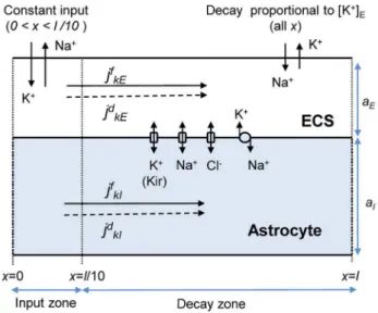
Figure 3. Astrocyte model.A representative astrocyte (I) exchanging ions with the ECS (E). As indicated, ions could cross the astrocytic membrane via passive Na+or Cl2channels, via the K+Kir channel or the Na+/K+-pump. Ions could also be transported longitudinally by electrical migrationjfknor diffusionjd
knthrough the ICS (n~I) or ECS (n~E). The cation-exchange input was a constant influx of K+and efflux of Na+to/ from the ECS of theinput zone(defined as the region0vxvl=10). The cation-exchange output was an efflux of K+and influx Na+from/to the ECS. The output was proportional to the local K+-concentration, and occurred over the whole axis. Thedecay zonewas defined as the part of the axis where no input was applied (xwl=10), i.e., the region where there was a net efflux of K+from the system.
doi:10.1371/journal.pcbi.1003386.g003
Table 2.Model parameters.
Parameter Value Reference
l(length of astrocyte) 300mm
DK(K+diffusion constant) 1:96|10{9m2=s [31,36,37]
DNa(Na+diffusion constant) 1:33|10{9m2=s [31,36,37]
DCl(Cl2diffusion constant) 2:03|10{9m2=s [31,36,37]
lI(intracellular tortuosity) 3.2 [12]
lE(extracellular tortuosity) 1.6 [12]
CM(specific membrane capacitance) 1mF=cm2 [38]
gK0(baseline K+-conductance) 16:96 S=m2 [38]
gNa0(baseline Na+-conductance) 1 S=m2 [38]
gCl0(baseline Cl–conductance) 0:5 S=m2 [38]
Pmax(maximum Na+/K+pump-rate) 1:12|10{6mol=(m2s) [20]
KKE(½KzE-threshold for Na
+/K+pump)
1:5 mol=m3 [20]
KNaI(½NazI-threshold for Na+/K+pump) 10 mol=m3 [20]
½Kz0
E(initial ECS K+-concentration) 3:0z0:082 mM
* [20]
½Kz0
I(initial ICS K
+-concentration) 100:0{0:041 mM* [20]
½Naz0
E(initial ECS Na+-concentration) 145:0{0:378 mM
* [20]
½Naz
0I(initial ICS Na+-concentration) 15:0z0:189 mM
* [20]
½Cl{0
E(initial ECS Cl–concentration) 134:0{0:29 mM
* [20]
½Cl{0
I(initial ICS Cl–concentration) 5:0z0:145 mM
* [20]
vM0
*(initial membrane potential) {
85z1:4 mV [20]
kdec
{
(decay factor for½Kz
E) 2:9|10{8m=s [54]
jin(constant input in input zone) 7|10{8mol=(m2s)
*Initial concentrations are given as½k0
n~Value from½20+Correction, where the sum gives the baseline (resting) concentration in the default
parametrization of the model.
{The maximum average Na+/K+-pump rate for a single neuron was estimated to A~2|10{7mol=(m2s)[54]. We obtainedk
decby solving
kdec(½KzmaxE {½K z0
E)~A, assuming that½K zmax
jout
K ~{jNaout~{kdec(½KzE{½K
z0
E) for allx ð31Þ
The decay factor (kdec) was set to a realistic value for maximal neuronal Na+/K+-exchange under physiological conditions (see Table 2). The input flux density reflected the activity level of local highly-active neurons. In our simulations, we specified jin to a value that gave a K+-concentration of about 10 mM in the input zone during constant input (see Results for details). This concentration level is on the critical threshold between functional and pathological conditions [3,12,21], and should thus represent a case where the spatial buffering process plays a critical role.
We note that the distinction between an input and an output flux density had a practical motivation, as we wanted to to distinguish between processes causing K+ to enter/leave the system (we could instead have defined a net input asjin{jout). We also note that both the input and output were cation-exchanges, and thus did not introduce any net charge to the system (cf. Eq. 28).
Astrocytic membrane mechanisms. Four selected astro-cytic membrane mechanisms were adopted from a previous point-model of an astrocyte [38]. The included mechanisms were standard, passive Na+and Cl2channels, the inward rectifying K+ -channel (Kir), and the Na+/K+-pump, as sketched in Fig. 3. The transmembrane ion fluxes in the astrocyte model were:
jKM~ gKfKir
F ðvM{eKÞ{2P ð32Þ
jNaM~ gNa
F ðvM{eNaÞz3P ð33Þ
jClM~{ gCl
F ðvM{eClÞ: ð34Þ
Here,gk are the passive conductances of the K+(Kir), Na+and Cl2 channels. The currents depend linearly on the difference
betweenvM and the reversal potential,
ek~ylog(½kE=½kI), ð35Þ
for the respective ion types (k). The potassium current was modified by the Kir-function [12]:
fKir(½KzE,Dv,vM)~ ffiffiffiffiffiffiffiffiffiffiffi
½Kz
E
½Kz0
E r
1zexp(18:4=42:4) 1zexp½(Dvz18:5)=42:5
h i 1zexp½{(118:6zeK0)=44:1
1zexp½{(118:6zvM)=44:1
h i ð36Þ
where Dv~vM{eK, andeK0 is the Nernst potential for K+ at
basal concentrations½Kz
0E and½Kz 0I.
The K+/Na+-pump uses energy (ATPase) to exchange 2 potassium ions with 3 sodium ions. We used a pump-rate per unit area defined by:
P(½Naz
I,½K
z
E)~Pmax
(½Naz
I)
1:5
(½Naz
I)
1:5zK1:5
NaI
½Kz
E ½Kz
EzKKE : ð37Þ
The maximum pump rate, Pmax, and the threshold concentra-tions,KNaI andKKE, are given in Table 2.
Initial conditions. Initial conditions were determined in the following way: As a starting point, we used ½k0n~½kLn and vM0~vMLas our initial conditions, where½kLn andvMLwere the resting concentrations and resting membrane potential found in a previous study [20]. We then ran a simulation with no system input or output. With the membrane mechanisms included in Eqs. 32–34, the system had a simulated resting state (½kSn and vMS) which was close to, but not identical with½kLn and vML. For all subsequent simulations, we set the initial conditions to the simulated resting conditions (½k0n~½kSn and vM0~vMS). The estimated values and the values from the literature are given in Table 2.
Prior to all simulations, we defined the static charge densities:
rsI~OM aI
CMvM0{F(½Kz0Iz½Na
z 0I{½Cl{
0I) ð38Þ
rsE~{OM aE
CMvM0{F(½Kz0Ez½Na
z
0E{½Cl{
0E): ð39Þ
The static charge densities ensure that the total charge density inI andEare consistent withvM0, according to Eq. 7.
Comparison of concentrations and charges. To allow direct comparison with ion concentrations, we represent the charge density in Eq. 7 as an equivalent concentration of unit charges, defined by:
½ez n~½Kz
nz½Naz
n{½Cl{
nzrsn=F, ð40Þ
with Eq. 38 or Eq. 39 forrns. Likewise, we represent the current densities as equivalent unit-charge flux densities, defined by:
jenf ~j f Knzj
f Nan{j
f
Cln ð41Þ
jend~jdKnzjNand {jdCln ð42Þ
Implementation. The model was implemented in Matlab, and the code will be made publicly available at ModelDB (http:// senselab.med.yale.edu/modeldb). Simulations were run using the Matlab-solver pdepe, which uses variable time steps. For the simulations presented below, we used a maximum time step of 0.1 s, and used 100 segments in the x-direction. A single simulation (e.g., producing Figs. 4 and 5) then took about 1 min to run on a standard laptop. Improving the resolution had no visible impact on the predicted results. Initial conditions were as listed in Table 2, and the sealed-end boundary conditions (Eq. 6) were applied.
Results
Here, we have applied the formalism to simulate spatial K+ -buffering by astrocytes, using the specific implication to the atrocyte/ ECS-model, also presented in the Model section. Our main objective has been to investigate the transport routes of K+ions, from entering the system in the ECS of the input zone, to leaving the system at some point along thex-axis. We remind the reader that a useful list of symbols and definitions can be found in Table 1.
Ion concentration dynamics in the Astrocyte/ECS system We investigated the ion concentration dynamics in the astrocyte model (Fig. 3) in full detail. Fig. 4A–D shows the dynamics of selected variables in the input zone (at x~0). Fig. 4E–H shows how the same variables depend onxat a timetSS~400 swhen the system was in SS. We explain this further below.
The input was applied fromt~100 stot~400 sin the input zone (0vxvl=10~0:03 mm). This is illustrated in Fig. 4A(solid line), which shows the flux density of K+(jin
K) entering the system in the input zone. We recall that the input was a cation exchange, so that there was an equal flux density of Na+leaving the system
Figure 4. Dynamics and steady state profiles for the astrocyte/ ECS-system.(A–D) Dynamics of selected variables in a point (x~0) in the input zone. (E–H) Spatial profiles of selected variables at a time
t~400 s, when the system was in steady state. The constant cation-exchange input was applied to the ECS of the input (0vxv0:03 mm) zone fromt~100 stot~400 s. (A) The input and output flux densities of K+to the pointx~0. We recall that the Na+input/output (not shown) was the opposite of that of K+:jin
Na~{jinKandjNaout~{jKout. (B,D) During the input, ion concentrations in the ECS and ICS changed, but reached steady state after about 10–50 s after stimulus onset. (B) ½Kz
E (at
x~0) had then increased by about 7.7 mM with respect to the baseline value. (C)½Kz
Ihad increased by about 12.5 mM due to uptake by the astrocyte. (D) The astrocytic membrane potential had been depolarized to about259 mV atx~0. The impact of the input was smaller outside
the input zone. (F–H) Deviations from the baseline ionic concentrations and vM typically decreased with x. Far away from the input zone (x~0:3 mm), the conditions were close to the baseline conditions. (B–C, F–G) Ionic concentrations were represented in terms of deviations from resting concentrations: D½kn~½kn{½k
0
n for n~I,E. For direct com-parison with ion concentrations, the charge density was represented as an equivalent concentration of unit charges½ez
n. doi:10.1371/journal.pcbi.1003386.g004
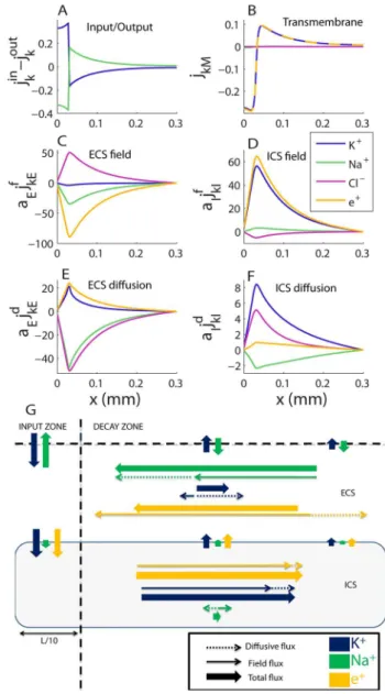
Figure 5. Transports in the astrocyte/ECS system during steady state. (A) Total flux densities into system (input{output). (B) Transmembrane flux densities. (C–F) Longitudinal flux densities due to (C) electrical migration in the ECS, (D) electrical migration in the ICS, (E) diffusion in the ECS and (F) diffusion in the ICS. (A–D) To aid comparison, flux densitiesjknwere scaled by the relative area fractionan (e.g., ifaEjkE~aIjkI,IandEcarry the same the net flux of ion species k). (G) A flow chart that qualitatively summarizes the essential information in (A–F), showing the main transport routes of K+ and Na+during SS (Cl2excluded from the overview). K+generally entered the system in the input zone and left the system from some point along the astrocyte axis. The transport route of K+(from entering to leaving
the system) was predominantly intracellular, demonstrating the astrocyte’s efficiency as a spatial buffer. Na+entered in the decay zone and left from the input zone. Na+transport predominantly took place in the ECS. The illustration (G) is qualitative - longer arrows mean higher flux densities, but the mapping from (A–F) to (G) is not quantitatively exact. The input zone was in the region0vxv0:03 mm. Units on they -axis aremmol=(m2s)in all panels.
(jin
Na~{jKin). For simplicity,jinNawas not included in the figure, but we keep in mind that whenever K+entered/left the system, an equal amount of Na+left/entered. The cation-exchange input thus caused an increase in ½Kz
E and a decrease in ½Na
z
E in the input zone. This can be seen in Fig. 4B. The notation D½kn represents the deviations from baseline concentration (cf. Table 2).
As ½Kz
E increased, the output from the system (being proportional to ½Kz
E) increased. Also this is illustrated in Fig. 4A (dashed line), which shows the flux density of K+ (jout
K ) leaving the system from a pointx~0in the input zone. We recall that also the output was a cation exchange, so that the efflux of K+ implied a corresponding influx Na+.
The input was given in the input zone, while the output occurred over the full axis, depending on the local value of½Kz
E. During a transient period, the constant input changed the ion concentrations in the system. The system reached steady state (SS) when½Kz
E became sufficiently high. Then, the total amount of K+entering the system per second, and the total amount of K+ leaving the system per second, coincided (with the same being true for Na+). This is illustrated in Fig. 4E, which shows how thejin
Kand jout
K are distributed over thex-axis at a time t~400 s, when the system was in SS. The areas under the curves forjin
KandjKoutwere then equal. In the input zone, however, the output rate was about 1/3 of the input rate (Fig. 4A). This means that about 2/3 of the K+ that entered the system was transported in the positive x -direction, and left the system from the decay zone. (We recall from Fig. 3 that the decay zone is defined as any part of the x-axis outside the input-zone).
Fig. 4B–D shows how the local (at x~0) intracellular ion concentrations, the extracellular ion concentrations and vM changed from the input had been turned on until the system reached SS. For the present example it took 49 s from the constant input had been turned on until the slowest variable (D½Cl{
E) reached 99% of its SS value. The other variables approached SS faster than this (e.g., 12 s forD½Kz
E and 19 s forDvM). During SS,D½Kz
Ewas about 7.7 mM, corresponding to a concentration ½Kz
E^10:8 mM(as the baseline concentration was*3:1 mM). Although the input was applied to the ECS of the input zone, the local intracellular K+-concentration had increased even more (D½Kz
I^12:5 mM). This reflects the astrocyte’s propensity for local K+-uptake. The changes in ionic concentrations in the ECS and ICS coincided with a local depolarization of the astrocytic membrane, from the resting potential (vM0*{84 mV) to about
vM~{59 mV, reflecting concentration dependent changes in the reversal potentials of the involved ionic species.
From here on, we focus on the SS-situation, i.e., on the activity of astrocytes during periods of on-going intense neural activity. For all system variables, the devition from the baseline (resting) conditions were generally biggest at the pointx~0, i.e., in the part of the input zone which is furthest away from the decay zone (Fig. 4E–H). The average value of ½Kz
E, taken over the input zone (0vxv0:03 mm) was approximately 10 mM (about 6.9 mM above the resting concentration). During the model calibration, the constant input rate (jin) was tuned to obtain this value, which is on the threshold between functional and pathological conditions [3,12,21]. During SS, the gradients in ionic concentrations (Fig. 4F–G) andvM (Fig. 4H) were quite pronounced. We thus expect that both diffusive and electrical forces contribute to transporting ions through the system (from entering to leaving). This is explored further in the following section.
Ion transport pattern in steady state. Fig. 5 shows spatial profiles of all ionic flux densities during SS. As Fig. 5Ashows, there is a net external influx of K+(blue line) to the in the ECS of the
input zone (jin
K{jKoutw0), and a net external efflux of K+in the ECS of the decay zone (jin
K{jKoutv0). In the case of Na+, the situation is opposite.
We first focus on the transports of K+, from entering the system in the input zone (xv0:03 mm), to leaving from some point along the x-axis. From Fig. 5B we see that K+ is taken up by the astrocyte in the input zone (negativejKMrepresents an inward flux density), and released from the astrocyte to the ECS in the decay zone. This implies that there must be longitudinal transport of K+ inside the astrocyte, out from the input zone. The longitudinal flux densities are shown in Figs. 5C–F. We have distinguished between field flux densities (jknf ), driven by voltage gradients, and diffusive flux densities (jd
kn), driven by concentration gradients (cf. Eq. 4). In the ECS, the electrical migration of K+ (Fig. 5C) was in the negativexdirection, while diffusion was in the positivex-direction (Fig. 5E). Inside the astrocyte, diffusion and electrical migration were both in the positivex-direction (Figs. 5D, F). Transport of K+ in the positivex-direction (out from the input zone) therefore had the best conditions in the ICS.
In the case of Na+, the situation was different. Firstly, Na+ entered the system in the decay zone of the ECS, and left the system from the input zone (Fig. 5A). The transmembrane Na+ -flux was very small (Fig. 5B), and the main longitudinal transport occurred in the ECS. As in the case of K+, electrical migration of Na+in the ECS, was in the negative x-direction. However, for Na+, this was also true for diffusion. Longitudinal transport of Na+ therefore had good conditions in the ECS, as diffusion and electrical migration both drove Na+in the same direction (towards the input zone).
The main transport routes K+ and Na+ during SS are summarized in Fig. 5G: K+ entered the system in the ECS of the input zone, where a major fraction of it crossed the membrane. Transport of K+out from the input zone predominantly took place inside the astrocyte. Outside the input zone (i.e., in the decay zone), the astrocyte released K+ to the ECS, from where it eventually left the system. Na+, on the other hand, entered the system in the decay zone, and was predominantly transported longitudinally through the ECS before leaving the system from the input zone. The net Cl2transport (jd
ClEzj f
ClE) was very small (flux densities due to diffusion and electrical migration canceled each others out), and was not included in the summary.
Two basic mechanisms explain the qualitative difference between Na+and K+transports. Both are related to the membrane being most depolarized in the input zone (Fig. 4F). The first mechanism concerns the axial fluxes. As the astrocyte was most depolarized in the input zone, the charge density (positive in the ICS and negative in the ECS) had the highest absolute value there. Therefore, the electrical forces on K+and Na+(being cations) were in the negativex-direction in the ECS (LVE=Lxw0), and in the positive x-direction in the ICS (LVI=Lxv0). This favoured the ICS for transporting K+ away from the input zone, while it favoured the ECS for transporting Na+ into the input zone. Furthermore, this finding predicts that the astrocyte not only provides an additional and more effective domain for longitudinal K+-transport, but even reduces the net transport of K+through the ECS. To our knowledge, we are the first to suggest that astrocytes may use this mechanism for shielding the ECS from K+.
The second mechanism for explaining the differences between the Na+and K+ transports concerns the transmembrane fluxes. The Na+/K+-pump mediated an inward flux of Kz
astrocyte. These passive fluxes were proportional to the deviation between vM and the reversal potential (vM{ek). In the case of Na+, the passive flux and the pump rate were locally closely balanced across the length of the astrocyte (results not shown). The transmembrane Na+-flux was therefore small everywhere (Fig. 5F). During SS, the Kir-reversal potential was more negative thanvM at all points along thex-axis (Fig. 6A). Therefore, Kir exclusively conducted an outward K+-flux. However, this outward flux was small in the input zone, where the Kir-reversal potentialeK was close to vM. In the input zone, therefore, the Na+/K+-pump dominated, giving rise to a net K+-uptake by the astrocyte (Fig. 6B). Outside the input zone, Kz
-release through the outward Kir-channel dominated. These simulations support the prevailing view that in the context of spatial buffering, Kir mainly mediates an outward current, and that the main uptake is due to the Na+/K+ -pump (see reviews in [3,25]).
Sensitivity analysis. The qualitative model performance was robust to parameter variations. Fig. 7 shows the sensitivity of the peak K+-concentration in the ECS during SS (½Kz
maxE ) to variations in selected model parameters. All peak values occurred atx~0.
As expected,½Kz
maxE depended on the balance between the input rate (jin) and decay factor (kdec). Fig. 7Ashows that½KzmaxE increased with increasing jin and decreased with increasingkdec.
The default parameter values (see Table 2) are indicated with a black circle, while green and red circles indicate two other combinations ofjin and kdec which gave similar peak amplitudes (½Kzmax
E ^10:8 mM) atx~0. ½Kzmax
E increased smoothly with increasing input zone length (liz) (Fig. 7B). The sensitivity to the tortuosities (lEandlI) was also as expected (Fig. 7C–D). Increasinglncorresponds to decreasing the effective diffusion constant (Dk=l2n), and thus had a negative impact on the system’s ability to buffer K+spatially.
Variations in the membrane parameters (gK,gNa,gClandPmax) led to changes, not only in ½Kzmax
E , but also in the baseline concentration (½Kz0
E) prior to the input (Fig. 7E–H). As long as the parameters were kept reasonably close (within+50%) to the default parameter values, the system behaviour was qualitatively similar to that observed in Figs. 4 and 5. The sensitivity togCl0was
low.
The high sensitivity toPmax (Fig. 7H) can be understood quite intuitively: An increased Na+/K+-pump rate led to more K+ leaving the astrocyte, and thus an increased ECS concentration. The sensitivity togNa(Fig. 7F) has a more indirect interpretation: When gNa was decreased, the passive Na+ current into the astrocyte decreased, and the outward current through the Na+/ K+-pump led to a hyperpolarization of the astrocyte. For example, with gNa~0:5 S=m2, the resting membrane potential was vM~{104 mV. An equilibrium between K+influx through the pump and efflux through the Kir-channel then required a corresponding hyperpolarization of the K+ reversal potential (eK), i.e., an increase of½KzI on behalf of½K
z
E (cf. Eq. 35). The sensitivity of½Kzmax
E and½K
z0
E to variations ingK was low (Fig. 7E). This, somehow counterintuitive, finding was likely due to the Kir-channel being the most abundant membrane mechanism, with gK being about 17 times as high as gNa by default. Despite moderate variations ofgK,vM therefore always resided relatively close toeK (results not shown). A low sensitivity to pharmacological intervention with astrocytic Kir-channels has also been found experimentally [39]. In our simulations, however, a further reduction of gK (below the parameter range in 7E), caused½Kz0
E to drop rapidly towards 0, where the mathematical system is singular. We did not explore this effect further, but note that egn. 36 for the Kir-channel was empirically determined for retinal Mu¨uller cells [12,21], and it is questionable whether it is applicable at extreme parameter values (i.e., extremely low concentrations).
Electroneutrality. It has been previously withheld that to preserve electroneutrality, an influx of K+from the ECS to the glia cell must be accompanied with an influx of an anion (such as Cl2)
or an efflux of another cation (such as Na+) [30]. Physically, however, the system is not strictly locally electroneutral in the thin Debye-layer surrounding the capacitive membrane. Before the system reaches steady state, there must be a net transfer of charge into the astrocyte, consistent with the depolarization of the membrane.
A consistent relationship betweenvM and ionic concentrations is implicit in the electrodiffusive formalism presented here. To get an insight in the relationship betweenvM and ionic concentration, we have presented the charge density in Fig. 4 as an equivalent concentration of positive unit charges ½ez
(cf. Eq. 40). In the astrocyte model, the resting potentialvM0~{83:6 mV
correspond-ed to concentrations½ez
E^0:36 mMand½e
z
I^{0:18 mM(the negative concentration of ez
unit charges could be read as a positive concentration of negative unit charges e{
.) Physically (although this is not explicit in a one dimensional model) this represents the charges stuck on both sides of the membrane. These
Figure 6. Membrane mechanisms involved in spatial K+
-buffering.(A) The K+reversal potential (e
K) was more negative than vM at all points along the x-axis. The Kir-channel thus exclusively mediated an outward K+-current. (B) In the input zonee
are equal in magnitude, but have opposite signs (the concentrations differ by a factor 2 due to the ICS having twice the volume of the ECS). At SS,vM had increased from the resting potential to about 260 mV, consistent with small absolute changes (D½e{I^
0:05 mM and D½e{
E^0:10 mM) in the concentration of unit charges. As seen in Fig. 4B–C, these changes were very small compared to the changesD½kin any of the ionic concentrations. Anions and cations were thus always closely balanced in numbers, reflecting the nearly electroneutral nature of the system.
Only when the system had reached SS (and the capacitive currentLvM=Ltwas zero), the net charge crossing the membrane was zero. However, this applied to the astrocyte as a whole, and was not locally true. During SS, there was a net influx of charge in the input zone due to the large uptake of K+there. This is evident in Fig. 5F, where net electrical currents have been represented as equivalent flux densities of unit charges (cf. Eqs. 41–42). This did not lead to any accumulation of charge inside the astrocyte, as the charge that entering was transported intracellularly out from the input zone (Fig. 5B,D) before being re-released to the ECS in the decay-zone (Fig. 5F). During SS, the sum of the Na+ and K+ transports gave rise to a net electrical current which cycled in the system (Fig. 5G).
We also add a remark regarding the limitations of standard cable theory. In standard cable theory, diffusive currents are assumed to have a negligible impact on vM, and intra- and extracellular resistivities are assumed to be constant (i.e., not dependent on ion concentration variations). During our simula-tions ionic concentrasimula-tions changed by several mM before the system reached SS (Fig. 4). These changes corresponded to a 10% decrease and 20% increase, respectively, in the intra- and extracellular resistivities (cf. Eq. 15, results not shown). Further-more, Fig. 5 showed that the diffusive current contributed quite significantly to the net electrical transport, and was about 25–30% of the field current in the ECS. Hence, for the process simulated here, standard cable theory would give relatively poor predictions ofvM.
The relative importance of spatial buffering in K+ -clearance
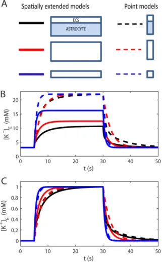
In addition to spatial buffering, K+may also be buffered by diffusion through the ECS alone, or by local (space independent) storage by the glial cell, to be later released in the same region of the ECS [19,24]. To investigate the relative importance these clearance mechanisms, we compared the 6 six model versions depicted in Fig. 8A, including one group of three spatially extended models (solid lines), and one group of three point models (dashed lines). Both groups included one model version with an active astrocyte, one model version where the astrocyte had been replaced by a corresponding increase in the ECS volume (the total ECS volume fraction increased toaE~0:6), and one version where the original ECS volume fraction (aE~0:2) was kept when the astrocyte was removed. The spatially extended model including the astrocyte, is the one we studied in the previous sections. The other models were reduced versions of this.
All model versions were exposed to the input signal described by Eq. 30, causing an increase in½Kz
E. The input was applied in the time window5svtv40 s, which was sufficient for½Kz
Eto reach its SS-value in all models. Fig. 8Bshows the dynamics of the K+ -concentration in the ECS at the point where the -concentration was the highest (½Kzmax
E ). In the spatially extended models, this occurred atx~0, i.e. in the part of the input zone furthest away from the decay zone.
During SS, the net K+efflux and influx from/to the system coincided. For the point models, having no spatial resolution, there was no distinction between the input zone and decay zone, as the input and output were injected to/subtracted from the same single compartment. The net output rate thus depended on½Kz
Ein this single compartment. Therefore, all point models approached the same SS value (½Kzmax
E &22 mM). For the spatially extended models ½Kzmax
E was lower, as parts of the K+could leave the system also outside the input zone. For these models, ½Kzmax
E
Figure 7. Sensitivity analysis.Sensitivity of½Kz
maxE (maximal extracellular½Kz
in the input zone) to variation in selected model parameters. (A) Sensitivity to input flux density (jin) and the output rate constant (kdec). Similar values of½KzmaxE &11 mMwere obtained for the three marked data points: (i) black:kdec~2:9|10{8m=s,jin~5:5|10{8mol=(m2s)(default conditions), (ii) green:kdec~1|10{8m=s,jin~3|10{8mol=(m2s), and (iii) red:kdec~5|10{8m=s,jin~8|10{8mol=(m2s). B–D) Sensitivity to the length of the input zone (liz), and tortuosities in the ECS (lE) and ICS (lI). (E– H) Sensitivity of½Kz
maxE and½K z
0E(baseline extracellular½K z
) to membrane conductances (gK,gNaandgCl), and the maximal Na+/K+-pump rate (Pmax).D½KzE~½K
z
maxE (i){½Kz
0E. (B–H) The legend applies to all panels. Black (i), red (ii) and green (iii) lines correspond to the input-parameter combinations marked in (A).
depended on how efficient they were in longitudinally transporting K+out from input zone before (revisit Fig. 4 for more details).
To gain insight in the importance of local K+-uptake by astrocytes, relative to diffusion in the ECS, we compared the performance of the point model including the astrocyte (black, dashed line in Fig. 8B) to that of the spatially extended model including only the ECS (blue, full line). During the first few seconds after the stimulus had been turned on, the point model with the astrocyte (representing local uptake) was most efficient in terms of limiting½Kz
E. However, local uptake was limited by the storing capacitance of the astrocyte. After seconds with constant K+-influx to the system, the spatially extended model (representing diffusion through the ECS) performed better, as it could redistribute K+over a larger spatial region. The astrocyte’s ability to locally store excess K+has been emphasized in previous investigations [19,24]. Our simulations predicted that the local storage mechanism is mainly important in relatively short time spans after potassium release (a few seconds). A similar conclusion
was also drawn from previous modelling studies [10,12]. We here add an additional point to this discussion: The performance of the point model with extended ECS (dashed red lines) more or less coincided with that of the point model including the astrocyte (dashed black lines). In terms of local storage, the astrocyte (with its membrane being highly permeable to K+), essentially just acts to expand the local volume that the incoming flux of K+enters into.
It has been argued that because K+-transport is aided by transmembrane processes as well as internal processes in the glial cell, K+can be cleared more effectively by glia than would be possible by a much enlarged extracellular space [40]. To investigate this claim, we compared the three spatially extended models (solid lines). We found that the model including the astrocyte (black, solid line) was more successful in limiting½Kzmax
E than any of the other model versions. It was significantly more successful than diffusion in the ECS alone, even in the (rather hypothetical) system where the extracellular volume had been increased by a factor 3.
In conclusion: In terms of local storage, the astrocyte was not significantly more efficient than an increased enlarged extracellu-lar space. In terms of spatial buffering, however, it was.
Consistency of formalism. In all our simulations, vM was defined in terms of the charge density in I, and computed algebraically by solving Eq. 19 at each time step. Identical results (down to a very small numerical error) were obtained whenvM was defined by the charge density inE(Eq. 20), and whenvMwas computed differentially by using Eq. 29 (results not shown). As all transports are included in Eq. 29, the algebraic and differential methods yielded consistent results.
When the input was turned on and off, a small numerical error was introduced in the conservation of ionic concentrations, inducing a small error in the total charge in the system. The relative deviation from global charge neutrality (Qtot~0), defined asQtot~Qtot=(DQEDzDQID), whereQI and QE refer to the total charge inI andE, was about10{10. This gave rise to a relative
deviation from perfect charge symmetry (cf. Eq. 18), defined as
Er~(aIrI{aErE)=(DaIrIDzDaErED), which was also on the order of10{10 (for all x). Accordingly, v
M computed from the charge density in E deviated by a relative factor *10{10 from v
M computed from the charge density inI. This corresponded to an absolute difference of *10{8mV. Errors were larger, but still
small, when the differential method was used. ThenvM deviated locally by up to *10{6mV from v
M derived from the charge density inI orE.
Errors will generally depend strongly on the algorithm used for solving the differential equations, the time step, and the number of compartments in the simulated system. The errors could likely be reduced by using a smoother input signal than the step function in Eq. 30. We did not engage in further analysis of the origin of the errors, as we were content with their smallness in relation to the questions addressed here.
Discussion
We presented a one-dimensional, electrodiffusive framework for modeling the dynamics of the membrane potential (vM) and the ion concentrations(½kn)of all included ion species(k)in an intra- and extracellular domain (Fig. 2). The framework could have a broad range of applications within the field of computational neuroscience. In the current work, it was applied to simulate the role of astrocytes in K+-removal from high concentration regions.
Figure 8. Model comparison.(A) Six model versions, three spatially extended models (solid lines), and three point models (dashed lines). Two versions (black lines) included an active astrocyte. In two versions (red lines), the astrocyte volume had been exchanged with an enhanced ECS (the total ECS volume fraction increased toaE~0:6). In two versions (blue lines), the original ECS volume fraction (aE~0:2) was kept when the astrocyte was removed. (B) The performance of the six model versions were compared in terms of maximal½Kz
Ein the input zone during a constant K+influx to the system. (C) To compare the time course of the½Kz
Edynamics, the responses (in B) were normalized to the peak amplitude for each respective trace.