Behavior of Linear Beam-Plasma Instabilities in the Presence
of Finite Amplitude Circularly Polarized Waves
L. Gomberoff,
Depto. de F´ısica, Facultad de Ciencias, Universidad de Chile, Casilla 653, Santiago, Chile. ([email protected])
J. Hoyos,
Depto. de F´ısica, Facultad de Ciencias, Universidad de Chile, Casilla 653, Santiago, Chile. ([email protected])
and A. L. Brinca
Centro de F´ısica de Plasmas, Instituto Superior T´ecnico, 1049-001 Lisboa, Portugal. ([email protected]) Received on 11 December, 2004; revised version received on 22 April, 2004
We review the effect of finite amplitude circularly polarized waves on the behavior of linear ion-beam plasma instabilities. It has been shown that left-hand polarized waves can stabilize linear right-handed instabilities [1]. It has also been shown that for beam velocities capable of destabilizing left-handed waves, left-hand polarized large amplitude waves can also stabilize these waves. On the other hand, when the large amplitude wave is right-hand polarized, they can either stabilize or destabilize right-handed instabilities depending on the wave frequency and beam speed [2]. Finally, we show that the presence of large amplitude left-hand polarized waves can also trigger electrostatic ion-acoustic instabilities by forcing the phase velocities of two ion acoutic waves to become equal, above a threshold amplitude value.
1
Introduction
The nonlinear stability of finite amplitude circularly polari-zed electromagnetic waves in ion beam-plasma systems has been thoroughly studied through the years [3, 4] because of its importance in several space plasma environments and la-boratory plasmas [3, 4, 5, 6, 7, 8]. Parametric wave-wave interactions of circularly polarized electromagnetic waves in a plasma involving alpha particles drifting relative to the proton, have been studied by [9, 10, 11]. Their nonlinear evolution has also been studied by using drift kinetic effects [12] and hybrid computer simulation techniques[13]. Stu-dies have been carried out by [14, 15, 16], including the ef-fects of dissipation and of the beam drift speed. The effect and the evolution of the beam for right and left handed pola-rized waves, have also been studied by using simulation ex-periments [17]. These studies have considered linearly sta-ble systems[9, 10, 14, 15, 16]. Proton beams observed in the solar wind display large drift velocities which can be larger than the necessary velocity to generate a linear beam-plasma instability [18]. In [1], it was found that the behavior of li-near electromagnetic right-handed polarized instabilities (r-instabilities) in a beam-plasma system can be affected by the presence of a finite amplitude left-handed polarized wave (L-wave). It was also shown that r-instabilities can be stabi-lized by L-waves in a linearly unstable proton beam-plasma system. These results were confirmed by using computer simulations [19], where it was also argued that the observa-tional results of [18] could be explained by the presence of
a large amplitude L-wave.
We also show here that the presence of an L-wave trig-gers electrostatic instabilities above a threshold amplitude. These instabilities occurs when the phase velocities of two sound waves are equal [9, 10, 20]. These authors have shown that when the ion acoustic wave phase velocity of the sound waves moving forward relative to the proton back-ground and backward in the frame of the alpha particle be-come equal, they trigger electrostatic instabilities between these two modes. They also notice that the presence of a large amplitude L-wave can partially stabilize the electros-tatic instability [9, 10, 20]. Here we show that even if ini-tially the ion-acoustic waves moving forward and backward relative to the background proton core are stable, the pre-sence of a large amplitude L-wave can force the phase velo-cities to become equal, triggering thereby, the electrostatic instability. In this sense the presence of the large amplitude wave can also affect the properties of the linear electrostatic streaming acoustic waves for an L-wave amplitude above a threshold value.
ases with increasing L-wave frequency. For larger beam drift speeds, L-waves can also stabilize the left-hand pola-rized instability (l-instability). The mechanism is more ef-ficient for L-wave frequencies closer to the proton gyrofre-quency. In the case when there is a R-wave in the system, it is shown that the part of the linear unstable spectrum be-low the wave frequency (which, depending on the beam drift velocity, may involve right as well as left-handed instabili-ties) can be completely stabilized for pump wave amplitudes above a threshold value. It is also shown that the presence of R-waves produce the same stabilization effect on the li-near r-instabilities. We have also found that the presence of a L-wave produces electrostatic instabilities above a th-reshold amplitude. These instabilities occur when the phase velocities of the forward and backward ion-acoustic sound waves supported by the background proton population be-come equal. The results are summarized and discussed in Section 4.
2
Dispersion Relation
The linear plasma dispersion relation for circularly polari-zed electromagnetic waves propagating in the direction of an external magnetic field in a system consisting of electrons, a proton core, and a proton beam, is given by [21, 22, 23, 24],
y02= x2
0
1−x0 +
η(x0−y0U)2
1−(x0−y0U), (1)
where x0 = ω0/Ωp, y0 = k0vA/Ωp, vA =
B0/(4πnpMp)1/2 is the Alfv´en speed, U = V /vA is the
normalized beam velocity,η = nb/nc is the beam density
relative to the core density,Ωp = qB0/cMp is the proton
gyrofrequency.
The dispersion relation, Eq. (1), is valid in a current-free plasma and in the reference frame where the proton core is at rest [22]. For an alpha particle beam the dispersion relation was first derived by using kinetic theory in the semi-cold ap-proximation [22], and later on by using fluid theory [9]. The dispersion relation for an arbitrary ion beam can be found in [21].
We now derive very briefly the nonlinear dispersion
re-We assume the plasma to be composed by electrons, back-ground protons, proton beam, and an L-wave propagating along the external background magnetic field. Each plasma component satisfies the following fluid equation of motion,
µ∂
∂t+~u·∇~
~u= ql
ml
µ
~ E+1
c~u×B~
− ∇~p
nlml
, (2)
where~uis the bulk velocity,qlthe electric charge, mlthe
mass,E~ andB~ the electric and magnetic field respectively, and p the pressure.
As pointed out before, the dispersion relation given by Eq. (1) was first derived by linearizing Vlasov’s equation [22], and using the semi-cold approximation. Later on, it was derived by using first order perturbation theory on the fluid Eqs. (2) for zero temperature[9]. Finally, it was also shown to be an exact solution of Eqs. (2) for zero pressure[11].
In order to derive the nonlinear dispersion relation, we follow a similar procedure to [9, 11]. Thus, we perturb the fluid Eqs. (2) including the left-hand polarized electromag-netic wave moving in the direction of the external magelectromag-netic field along the x-axis, as follows,
δux = Re[uexp(ikx−iωt)],
δEx = Re[ǫexp(ikx−iωt)],
δnp = n0Re[
uk ω−kV0x
exp(ikx−iωt)], (3)
whereV0x=V is the beam speed.
For quantities perpendicular to the external magnetic fi-eld we write,
δu⊥=u+exp(ik+x−iω+t) +u−exp(ik−x−iω−t),
δB⊥=b+exp(ik+x−iω+t) +b−exp(ik−x−iω−t),
δj⊥=j+exp(ik+x−iω+t) +j−exp(ik−x−iω−t), (4) whereu⊥=uy+iuz, and similarly forB⊥andj⊥. On the other hand,k± =k0±kandω± =ω0±ω, wherek0and
ω0 are the frequency and wavenumber of the pump wave, which satisfies the dispersion relation in Fig. 1.
−4 −3 −2 −1 0 1 2 3 4 0
0.2 0.4 0.6 0.8 1 1.2 1.4 1.6 1.8 2
x
y
−F −b (a)
−s +s +F
+b −sb
+sb +B
−B
−4 −3 −2 −1 0 1 2 3 4 0
0.2 0.4 0.6 0.8 1 1.2 1.4 1.6 1.8 2
x
y
−b −F
−F −b (b)
L+L−D+L+R−B−cc+L+R−bB−ccb+L−R+B++L−R+bB+b
+(B−ccB+b−B−ccbB+)(R−R+b−R−bR+)/D= 0. (5)
⌈
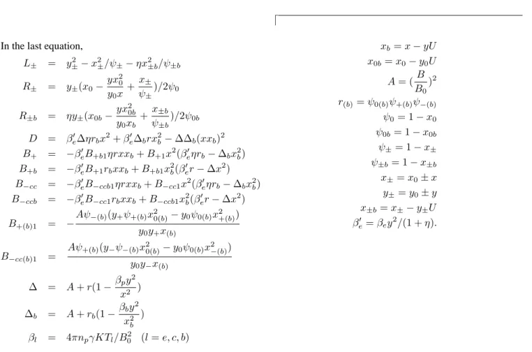
In the last equation,
L± = y2±−x2±/ψ±−ηx2±b/ψ±b
R± = y±(x0−yx
2 0 y0x+
x±
ψ±
)/2ψ0
R±b = ηy±(x0b−yx
2 0b
y0xb
+x±b
ψ±b
)/2ψ0b
D = β′
e∆ηrbx2+β′e∆brx2b−∆∆b(xxb)2
B+ = −β′eB+b1ηrxxb+B+1x2(β′eηrb−∆bx2b)
B+b = −β′eB+1rbxxb+B+b1x2b(βe′r−∆x2)
B−cc = −β′eB−ccb1ηrxxb+B−cc1x2(βe′ηrb−∆bx2b)
B−ccb = −β′eB−cc1rbxxb+B−ccb1x2b(βe′r−∆x2)
B+(b)1 = −
Aψ−(b)(y+ψ+(b)x20(b)−y0ψ0(b)x2+(b)) y0y+x(b)
B−cc(b)1 =
Aψ+(b)(y−ψ−(b)x0(2b)−y0ψ0(b)x2−(b)) y0y−x(b)
∆ = A+r(1−βpy
2
x2 )
∆b = A+rb(1−
βby2
x2
b
)
βl = 4πnpγKTl/B02 (l=e, c, b)
xb=x−yU
x0b=x0−y0U
A= (B
B0) 2
r(b)=ψ0(b)ψ+(b)ψ−(b) ψ0= 1−x0 ψ0b= 1−x0b
ψ±= 1−x±
ψ±b= 1−x±b
x±=x0±x
y±=y0±y
x±b=x±−y±U
βe′ =βey2/(1 +η).
TABLE 1. Characterization of the various modes appearing in Eq. (5). The + (-) sign refers to the upper (lower) sideband waves, and lh (rh)left-hand (right-hand) polarization. F refers to the branch of the pump wave, and b to the branch due to the beam.
+ (-) F lh (rh) forward propagating
+ (-) B rh (lh) backward propagating
+ (-) b lh (rh) forward propagating
+ (-) s ion-acoustic forward (backward) propagation + (-) sb beam ion-acoustic forward (backward) propagation
The finite amplitude wave is characterized by the coordi-natesx0andy0, and it is at the origin of the (x, y) coordinate system. For zero pump intensity,A= 0, Eq. (5) reduces to
L+L−D = 0. The solutionL± = 0, corresponds to the dispersion relation of the upper and lower side band waves, respectively. The other solutionD = 0, corresponds to the sound waves present in the system which, forη ≪ 1, are given by,
x≃ ±(βe+βp)1/2y, (6)
(x−yU)≃ ±(βb)1/2y, (7)
Eq. (6) corresponds to the ordinary ion-acoustic wa-ves propagating forward and backward relative to the
pro-ton core in the direcpro-ton of the magnetic field, and Eq. (7) corresponds to ion-acoustic waves supported mainly by the proton beam. They move forward and backward relative to the beam, along the external magnetic field. The solu-tions ofL± = 0 give the various branches of the disper-sion relation. The crossings between the solutions give the position and nature of the possible wave couplings of the system. The solutions of the nonlinear dispersion relation, Eq. (5), are invariant under a rotation through an angle of
180o. Therefore, it is sufficient to analyze the solutions in
(vth.ki =
p
2KTki/Mi) is the thermal velocity of
spe-cies i). This may happen either for small temperatures -and also for not so small temperatures[27, 21]- or for very large Alfv´en velocity relative to the thermal velocity, like e.g., in coronal holes [28, 29]. Eq. (5) corresponds to the disper-sion relation for L-waves. The disperdisper-sion relation for R-waves can be obtained by replacing (x, y) by (-x, -y) and
(x0, y0)by(−x0,−y0). Alternatively, one can simply take
(−x0,−y0) for the frequency and wavenumber of the R-wave and leave the rest unchanged. This is so because the (x, y) plane is invariant under rotations through an angle of 180o.
3
Graphical Analysis of the
Nonli-near Dispersion Relation
In order to study the nonlinear dispersion relation Eq. (5) we use a graphical method first used by [30].
3.1
Linear Instabilities in the presence of
L-waves
We start by studying the effect of varying proton-beam ve-locity on the stabilization of the linear r-instability due to the presence of an L-wave. In [1] it was shown that for
βi = 0.001, η = 0.2, U = 2, an L-wave of frequency
x0= 0.1stabilizes the linear r-instability forA= 0.16. As
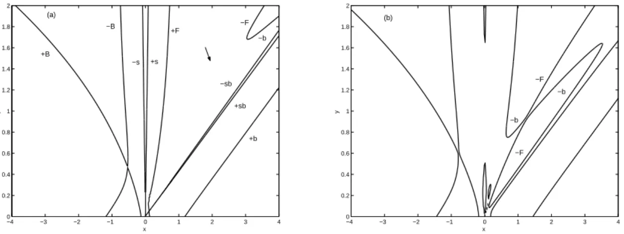
U increases,Atis expected to increase too. In Fig. 1a we
illustrate the situation for U = 2.3 andA = 0. The gap between the two curves denoted by -F and -b corresponds to the linear r-instability [1]. The lines denoted by -F and -b are lower R sideband waves propagating in the direction of the external magnetic field [1]. In Fig. 1b,A= 0.81and the gap between -F and -b has disappeared showing, thereby, complete stabilization of the linear r-instability. Thus, the threshold amplitude is nowAt= 0.81, instead ofAt= 0.16
forU = 2as expected,Atincreases with increasingU [1].
In Fig. 2a we have takenx0 = 0.5, andA = 0. The other parameters are the same as in the previous figure. In Fig. 2b, we have takenAt = 0.7, and the instability is
comple-tely stabilized. Thus, as the L-wave frequency increases, the thresholdAt-value decreases [1]. In general, for fixedU, the
instability threshold continues to decrease as the L-wave fre-quency approaches the proton gyrofrefre-quency. The effect is very pronounced for frequencies very close to the resonance. For example, forU = 3, andx0= 0.3,At= 2.5. However,
for the same drift velocity but forx0 = 0.95,At = 0.47.
Finally, in Fig. 3 we consider the case U = 2.8. In this case there are both r and l-instabilities. In Fig. 3a we have plotted the nonlinear dispersion relation forx0 = 0.9, and
A = 0. The arrow shows the linear instability region. In Fig. 3b,A = 0.63. The linear instability is completely sta-bilized. including the l-instability region corresponding to
the first to be stabilized asAincreases.
3.2
Linear Instabilities in the presence of
R-waves
We shall now study the effect of an R-wave on the linear instability. To do this, as explained above, one can simply choosex0to be negative and leave the rest unchanged. Thus, we take an R-wave of frequencyx0=−0.1. The other pa-rameters are the same as in Fig. 1. In Fig. 4a we illustrate the linear instability for A = 0andU = 2. This corres-ponds to the gap involving -F and -b. Note that these two roots correspond now to upper sideband waves while for an L-wave they correspond to lower sideband waves [1]. In Fig. 4b, At has been raised to A = 0.146. The gap has
disappeared altogether indicating complete stabilization of the linear r-instability. This is a similar situation to [1], but now the stabilization is due to the presence of an R-wave. We shall now increase the beam drift velocity to U = 4. As shown in Fig. 5a, there are several linear instability re-gions, r/l-instabilities. The region between B and C, and D and O are r-instabilities, while the region between O and G is l-instability. In the following we study the effect of a R-wave on these instability regions. To this end, we take
x0 = −0.1025, with correspondingy0 = −0.1. As it fol-lows from Fig. 5a, in this case the pump wave is unstable. In Fig. 5b we show the nonlinear dispersion relation, Eq. (5), forA= 0. The other parameters are like in the previous figures. There are two right-hand polarized instability regi-ons. One going from the origin to the point denoted by D, and the other from the C to B. The other two instability regi-ons cover the gap between the origin and the point denoted by G. In Fig. 5c, we have raised the pump wave amplitude toA= 0.1, and we see that, except for the region between the points D and C, the whole right hand branch has been destabilized. In Fig. 5d we have raised the pump wave am-plitude further toA = 0.21, and one can see that even the small stable region between D and C is now unstable. In other words, for a R-wave withA≥0.21the branch of the dispersion relation above the pump wave frequency is com-pletely destabilized. In this case the pump wave acts in the opposite direction than the left hand pump, i. e., it helps the destabilization of the this branch. For the same parameters of Fig. 5b, in Fig. 6a we show again the dispersion rela-tionxvs. y, and concentrate on the gap between the origin and the point denoted by G in Fig. 5a. This region invol-ves an r-instability which goes from the origin to the point
x= 0.1025andy = 0.1, and a l-instability going from this point to G. In Fig. 6b, the wave amplitude has been raised to
−6 −4 −2 0 2 4 6 0
0.5 1 1.5 2 2.5 3
x
y
−F −b (a)
−6 −4 −2 0 2 4 6
0 0.5 1 1.5 2 2.5 3
x
y
(b)
−b −F
−F
−b
Figure 2. Same as Fig. 1, butx0= 0.5for (a)A= 0, and (b)A= 0.7.
1 2 3 4 5 6 7 8 9 10 0
1 2 3 4 5 6 7
x
y
−F
−b (a)
1 2 3 4 5 6 7 8 9 10 0
1 2 3 4 5 6 7
x
y
−F
−b (b)
Figure 3. Nonlinear dispersion reltion, Eq. (3),xvs.y, forη= 0.2,U= 2.8,βi= 0.001,x0= 0.9, for (a)A= 0, and (b)A= 0.63.
−2 −1.5 −1 −0.5 0 0.5 1 1.5 2 0
0.1 0.2 0.3 0.4 0.5 0.6 0.7 0.8 0.9 1
x
y
−b −F (a)
−2 −1.5 −1 −0.5 0 0.5 1 1.5 2 0
0.1 0.2 0.3 0.4 0.5 0.6 0.7 0.8 0.9 1
x
y
−b −F (b)
−F −b
−20 −18 −16 −14 −12 −10 −8 −6 −4 −2 0 2 −6
−5 −4 −3 −2 −1 0 1 2 3 4
x0 y0
B C
D O G
−150 −10 −5 0 5 10 15 0.5
1 1.5 2 2.5 3 3.5
x
y
B
C
D G
−150 −10 −5 0 5 10 15 0.5
1 1.5 2 2.5 3 3.5 4
x
y
G D
C
(c)
−150 −10 −5 0 5 10 15 0.5
1 1.5 2 2.5 3 3.5 4
x
y
G (d)
Figure 5. (a) Linear dispersion relationx0vs.y0for a right-hand polarized pump wave withη= 0.2andU = 4. (b) Nonlinear dispersion
relationxvs.yfor a right-hand polarized pump wave of linearly unstable frequencyx0= 0.1025, withη= 0.2,βi= 0.001,U = 4and
A= 0, (c)A= 0.1, and (d)A= 0.21.
3.3
Electrostatic Instabilities in the presence
of L-waves
We now study the ordinary ion-acoustic waves given by Eqs. (6-7) in the presence of an L-wave. In Fig. 7a we show the nonlinear dispersion relation forx0 = 0.3with corres-pondingy0 = 0.4033for βi = 0.01 andA = 0, in this
case there is no instability regions associated with the ion-acoustic waves. In Fig. 7b we have raised the L-wave am-plitude toA = 0.293and the arrow in the figure indicates how the phase velocities of the ordinary ion-sound waves approach each other. In Fig. 7c we have raisedA= 0.3, the arrow in the figure shows it has appeared an instability re-gion that correspond to an interaction between these sound waves. This instability is electrostatic in origin and does not correspond to parametric decays of the large amplitude wave, because it does not involve modes associated with the band waves. The free energy source of this instability is de-rived from the kinetic energy of the proton beam. In general we have found that this instability appears for L-wave am-plitudes above a threshold amplitude.
4
Summary and Conclusions
By solving graphically the nonlinear dispersion relation Eq. (5) [30], we have shown the following properties of a system containing a finite amplitude circularly polarized wave
pro-pagating in a linearly unstable beam-plasma system. First, we assumed an L-wave and we showed that as the beam velocity increases the thresholdAt-value also increases. On
the other hand, for fixed drift velocity, the threshold required to stabilize the linear r-instability decreases with increasing pump wave frequency. In Fig. 8. the results are extended to various values ofβiand L-wave frequencies forU = 2.2
andU = 2.3. As it follows from Fig. 8,Atincreases with
increasing drift velocity, and decreases with increasing wave frequency for fixed drift velocity.
These results may have important applications. For example, [17] using hybrid simulations for a solar wind type plasma showed that the ion beam instability leads to a pro-ton beam anisotropyΓb = T⊥/Tk > 1[see Figs. 2a and 4a]. This result is consistent with previous similar studies for other space environments [3]. However, these results are in contradiction with the observations performed by [31] which show the opposite tendency, i. e.,Γb ≤1. One
pos-sible explanation for the discrepancy is the absence of large amplitude waves (see Figs. 2b-2c, and Fig. 3, and also Figs. 4b-4c, and Fig. 5).
−2 −1.5 −1 −0.5 0 0.5 1 1.5 2 0
0.1 0.2 0.3 0.4 0.5 0.6 0.7 0.8 0.9 1
x
y
G
(a)
−2 −1.5 −1 −0.5 0 0.5 1 1.5 2 0
0.1 0.2 0.3 0.4 0.5 0.6 0.7 0.8 0.9 1
x
y
(b)
G
−2 −1.5 −1 −0.5 0 0.5 1 1.5 2 0
0.1 0.2 0.3 0.4 0.5 0.6 0.7 0.8 0.9 1
x
y
G
(c)
Figure 6. Same as Fig. 5b for (a)A= 0, (b)A= 0.8, and (c) A= 1.35.
linear theory [4] and simulation experiments [17], the insta-bility must lead to a decrease of the drift velocity below the threshold value, and to an increase in the thermal anisotropy of the proton beam, i. e.,Γb >1. However, at least in the
case of Helios, some of the observations of the drift velocity lie above the instability threshold, 2 ≤U≤ 4. The persis-tence of these unstable distribution has been a problem awai-ting resolution [17]. In addition proton beams do not show a clear increase in the thermal anisotropy,Γb >1, [31]. If,
however, large amplitude left-handed waves are present in the system, the threshold beam drift velocity for linear ins-tability increases (relative to the threshold in the absence of large amplitude waves) rendering the system linearly stable [1].
−1 −0.8 −0.6 −0.4 −0.2 0 0.2 0.4 0.6 0.8 1 0
0.2 0.4 0.6 0.8 1 1.2 1.4 1.6 1.8 2
x
y
−S +S
(a)
−1 −0.8 −0.6 −0.4 −0.2 0 0.2 0.4 0.6 0.8 1 0
0.2 0.4 0.6 0.8 1 1.2 1.4 1.6 1.8 2
x
y
−S +S (b)
−1 −0.8 −0.6 −0.4 −0.2 0 0.2 0.4 0.6 0.8 1 0
0.2 0.4 0.6 0.8 1 1.2 1.4 1.6 1.8 2
x
y
(c)
−S +S
Figure 7. Dispersion Relation, Eq.(5), showing the ion acoustic waves (−S,+S) forU= 2.0,βi= 0.01,x0 = 0.3,y0= 0.4033,
(a)A= 0, (b)A= 0.293, the arrow in the figure indicates that the phase velocities of the ordinary ion-sound waves approach each other. (c)A = 0.3, the arrow in the figure shows the instability region corresponding to the electrostatic instability.
wave frequencies, andβi
η U x0 y0 βi At
0.2 2.0 0.001 0.00116 0.001 0.153 0.01 0.151 0.1 0.135 1.0 0.100 0.01 0.011581 0.001 0.151 0.01 0.150 0.1 0.134 1.0 0.110 0.1 0.112560 0.001 0.144 0.01 0.142 0.1 0.123 1.0 0.100
At increases with decreasing β. This behavior is similar
to the one encountered in the case of a L finite amplitude wave. On the other hand, the presence of the wave stabi-lizes the region between the pump wave frequency and O, and the region between O and G, forA≥At(see Fig. 6). In
this case, the finite amplitude wave can be triggered by the
A =At, the linear instability can be saturated by the same
wave triggered by the instability.
Thus, we have shown that a finite amplitude L/R-wave can act as a saturation mechanism for r/l hand polarized ins-tabilities. Another way of looking at these results is the fol-lowing. Linear beam-plasma electromagnetic instabilities behave in a different way in the presence of a finite ampli-tude L/R wave. For example, in the linear theory and in the absence of a finite amplitude wave, in order to trigger the r-instability, the drift velocity of a proton beam withη = 0.2
moving in the direction of an external magnetic field, must have a drift velocityU ≥1.95[24, 33]. However, the pre-sence of a finite amplitude polarized wave can stabilize the linear instability when the amplitude satisfiesA ≥At. For
the particular case whenU = 2.0with the other parameters like in Fig. 1, the system is completely stabilized in the pre-sence of a L-wave withAt≃0.16[1]. This result is shown
in Fig. 9a. This means that in the presence of the L-wave withA = 0.16, a larger beam drift velocity is required to trigger the r-instability. In fact, in Fig. 9b we have increased fromU = 2.0toU = 2.1in order to show that the insta-bility has reappeared. Of course ifA≫ At, a much larger
drift velocity is required to trigger the instability.
0 0.02 0.04 0.06 0.08 0.1 Β
0 0.2 0.4 0.6 0.8
At
U=2
U=2.2
U=2.3 HaL
0 0.2 0.4 0.6 0.8
x0 0
0.1 0.2 0.3 0.4 0.5
At
U=2
U=4 HbL
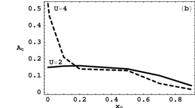
Figure 8. (a) Threshold L-wave amplitude,At, vs.βi, for fixedx0= 0.001and severalUvalues:U = 2.0(dashed line),U= 2.2(dotted
line), andU = 2.3(full line). (b) Threshold L-wave amplitude,At, vs. frequency,x0, for fixedβi = 0.01, andU = 2(full line), and
threshold R-wave amplitude for complete destabilization of the r-instability for the sameβibutU = 4(dashed line).
−2.50 −2 −1.5 −1 −0.5 0 0.5 1 1.5 2 2.5 0.5
1 1.5
x
y
−F
−b
−F −b (a)
−2.50 −2 −1.5 −1 −0.5 0 0.5 1 1.5 2 2.5 0.5
1 1.5
x
y
−F
−b
−F −b (b)
Figure 9. Same as Fig. 1, but for (a)U = 2.0andAt= 0.16, showing the stabilization of the linear right-hand instability, and (b)U = 2.1
Finally, in Fig. 7. we have shown the presence of an L-wave can trigger electrostatic instabilities. These insta-bilities occur when the phase velocities of two ion-acoustic waves become equal.
Acknowledgments
This work has been partially supported by FONDECYT grants 1020152 and 7020152. One of us (J. H.) thanks ME-CESUP for a doctoral fellowship.
References
[1] L. Gomberoff, J.Geophys.Res. 108 A6, 1261, doi: 10.1029/2003JA009387(2003).
[2] L. Gomberoff, J. Hoyos, and A. L. Brinca, J. Geophys. Res.
108, A12,1472, doi:10.1029/2002JA00576(2003).
[3] S. Gary, Space Sci. Rev. 56, 573 (1991).
[4] E. Marsch, Kinetic Theory of the Solar wind Plasma in The Physics of the inner Heliosphere, edited by E. Marsch and R.S. Schwenn. p.539, Pergamon, N. Y. (1991).
[5] M.M. Hoppe, C. T. Russell, L. A. Frank, T. E. Eastman, and E. W. Greenstadt, J. Geophys. Res. 86, 4471 (1981).
[6] M.M. Hoppe, C. T Russell, T. E. Eastmann, and L. A. Frank, J. Geophys. Res. 87, 643 (1982).
[7] M.D. Leubner, and A. Vi˜nas, J. Geophys. Res. 91, 13366 (1986).
[8] R.M.O. Galv˜ao, G. Gnavi, F. T. Gratton, and L. Gomberoff, Phys Rev. E. 54, 4112 (1996).
[9] J.V. Hollweg, R. Esser, and V. Jayanti, J. Geophys. Res. 98, 3491 (1993).
[10] V. Jayanti and J. Hollweg, J. Geophys. Res. 99, A12, 23449, doi: 10.129/94JA02370 (1994).
[11] L. Gomberoff, F. T. Gratton, and G. Gnavi, J. Geophys. Res.
99, 14, 717 (1994).
[12] B.A. Inhester, B. A., J. Geophys.Res. 95, 10, 525 (1990).
[13] V.J. Vasquez, J.Geophys. Res. 100, 1779 (1995).
[14] L. Gomberoff, J. Geophys. Res. 105, 10, 509 (2000).
[15] L. Gomberoff, K. Gomberoff, and A. L. Brinca, J. Geophys. Res. 106, 18, 713 (2001).
[16] L. Gomberoff, K. Gomberoff, and A. L. Brinca, J.Geophys. Res. 107, 1123, doi:10.1029/2001JA000265 (2002).
[17] W. Daughton, S. P. Gary, and Dan Winske, J. Geophys. Res.
104, 4657 (1999).
[18] E. Marsch, and S. Livi, J. Geophys. Res. 92, 7263 (1987).
[19] J. A. Araneda, J. A., and L. Gomberoff, J. Geophys. Res. 109, A01106,doi:10.1029/2003010189 (2004).
[20] V. Jayanti, and J. V. Hollweg, J. Geophys. Res. 98, 13, 247 (1994a).
[21] L. Gomberoff, L., IEEE Transactions on Plasma Science, 20, 843 (1992).
[22] L. Gomberoff, and R. Elgueta, J. Geophys. Res. 96, 9801 (1991).
[23] L. Gomberoff, and R. Hern´andez, J. Geophys. Res. 97, A8, 12, 113-12, 116 (1992).
[24] L. Gomberoff, and H. F. Astudillo, Planet. Space Sci. 46, 1683 (1998).
[25] L. Gomberoff, F. T. Gratton, and G. Gnavi, J. Geophys. Res.
100, 1871 (1995).
[26] L. Gomberoff, F. T. Gratton, and G. Gnavi, J. Geophys. Res.
99, 14, 717 (1994).
[27] L. Gomberoff, and R. Neira., J. Geophys. Res. 88, 2170 (1983).
[28] S. R. Cranmer, Space Sci. Rev. 101, 229 (2002).
[29] J. V. Hollweg, and P. A. Isenberg, J. Geophys. Res. 107, 1147, doi:10.1029/2001JA000270(2002).
[30] M. Longtin, and B. U. O. Sonnerup, J. Geophys. Res. 91, 6816 (1986).
[31] W. C. Feldman, J. T. Gosling, D. J. McMcComas, and J. L. Phillips, J. Geophys. Res. 98, 5593 (1993).
[32] B. E. Goldstein, N. Neugebauer, L. D. Zhang, and S. P. Gary, Geophys. Res. Lett. 27, 53 (2000).