Resumo
O que causou o declínio da produção de charque no Brasil? Sendo o principal alimento dos escra-vos, o charque era a indústria mais importante do sul do Brasil. No entanto, em 1850, produtores estavam preocupados porque não conseguiam competir com a indústria uruguaia. Interpreta-ções tradicionais atribuem o declínio a diferenças em produtividade entre os mercados de trabalho; pois enquanto o Brasil utilizava trabalho escravo, o Uruguai havia abolido a escravidão em 1842. Pesquisas recentes também levantam a possibili-dade de uma “doença holandesa” no Brasil, de-corrente do forte crescimento nas exportações de café. Ambas hipóteses são testadas e argumenta--se que o declínio da produção brasileira foi as-sociado a mudanças estruturais na demanda por carne de baixa qualidade. Políticas de proteção comercial criaram desincentivos para os produ-tores brasileiros aumentarem a produtividade e diversificar a indústria de carne.
Palavras-chave
doença holandesa; escravidão no Brasil, comércio do Uruguai.
Códigos JELN46; N56; O14.
Abstract
What caused the decline of beef jerky production in Brazil? The main sustenance for slaves, beef jerky was the most important industry in southern Brazil. Nevertheless, by 1850, producers were already worried that they could not compete with Uruguayan industry. Traditional interpretations attribute this decline to the differences in productivity between labor markets; indeed, Brazil utilized slave labor, whereas Uruguay had abolished slavery in 1842. Recent research also raises the possibility of a Brazilian “Dutch disease”,which resulted from the coffee export boom. We test both hypotheses and argue that Brazilian production’s decline was associated with structural changes in demand for low-quality meat. Trade protection policies created disincentives for Brazilian producers to increase productivity and diversify its cattle industry.
Keywords
Brazilian slavery; Dutch disease; Uruguay trade.
JEL CodesN46; N56; O14.
Thales A. Zamberlan Pereira Universidade de São Paulo
Was it Uruguay or coffee?
The causes of the
beef jerky industry’s decline in southern Brazil
(1850 – 1889)
1
Introduction
The cattle industry was the most important economic sector in southern Brazil during the nineteenth century. Beef jerky (charque) served as the main source of nourishment for enslaved laborers who worked on coffee and sugar cane plantations. Furthermore, between 1845 and 1889, it repre-sented on average 70.5 percent of Rio Grande do Sul province’s exports, along with hides (FEE, 2004). After the 1850s, nevertheless, local cattle ranchers and beef jerky exporters could not compete with Uruguayan pro-duction (Cardoso, 2003, p.204; Bell, 1998, p.79). This paper explores why the Brazilian beef jerky industry lagged behind despite the fact that Brazil had the largest slave population in the Americas after 1850.
Traditional interpretations attributed the lack of competitiveness to la-bor markets. These analyses credited as explanations for the stagnation in production differences in productivity between slave labor in Rio Grande do Sul and wage labor in Uruguay, as well as rising slave prices after the end of the transatlantic slave trade in 1850. Monasterio (2005), however, refuted the hypothesis that the use of slave labor was inefficient; he ar-gued that captives represented a lower cost than wage labor for beef jerky production. Monasterio raised an alternative hypothesis, suggesting that the coffee export boom damaged the southern industry through a “Dutch disease”: the real exchange rate appreciation caused by the soaring cof-fee exports raised Brazilian charque prices, making them less competitive against foreign competition.
The increased integration of Latin America into the world economy in the second half of the nineteenth century is well known (O’Rourke; Williamson,1999), but the impact of the first globalization on peripheral industries has yet to be thoroughly explored. Uruguay’s growth did not primarily arise out of increasing exports of beef jerky to Brazil; rather, its success resulted from the diversification of its exports. Regional military conflicts, especially the Paraguayan War (1864–1870) – also known as the War of the Triple Alliance – led to an increased demand for products that could be conditioned, such as canned beef. Moreover, shifting external demands from European markets created incentives to diversify production in Uruguay, which did not have a substantial internal market for its products. Brazilian producers, however, received a different set of incentives. With tariff protection offered by the government and a guaranteed market for its product, the southern Brazilian beef jerky industry did not have incentives to exchange their modes of production for more high-quality meats, since it would face international competition. Low wages in Brazil would make high-quality meat production unprofitable if producers relied solely on internal markets. Another important aspect of the Brazilian and Uruguayan cattle industries’ different approaches involved the supply of new technology. Uruguay’s modernization was built with British foreign capital. Southern Brazil, in the absence of foreign investments, lacked access to financial institutions that could make such modernization possible.
2
Beef jerky exports in Rio Grande Do Sul
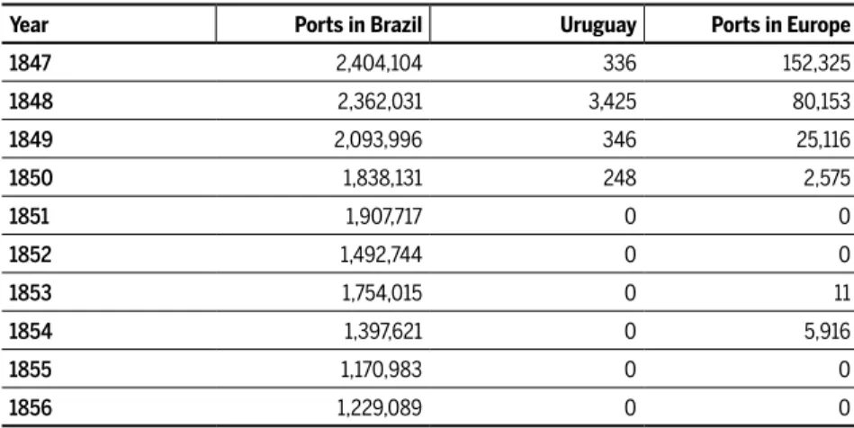
Report, 1857, p.35).1 Regarding beef jerky production in Rio Grande do Sul, as can be seen in Table 1, the majority of exports went to other ports in Brazil, such as Rio de Janeiro and Pernambuco, to feed slaves that wor-ked at the coffee and sugar cane plantations. Exports to ports in Europe, as Spain, Italy, and Portugal, represented a small portion of production.2
Table 1 Destination of Rio Grande do Sul beef jerky exports (arrobas)
Year Ports in Brazil Uruguay Ports in Europe
1847 2,404,104 336 152,325
1848 2,362,031 3,425 80,153
1849 2,093,996 346 25,116
1850 1,838,131 248 2,575
1851 1,907,717 0 0
1852 1,492,744 0 0
1853 1,754,015 0 11
1854 1,397,621 0 5,916
1855 1,170,983 0 0
1856 1,229,089 0 0
Source: Provincial Presidential Reports, Rio Grande do Sul (several years)
Notwithstanding the complaints from local producers quoted by Cardoso
(2003) and Bell (1998), two major political conflicts benefited Rio Grande do Sul’s beef jerky industry at the beginning of the 1850s. The first con-flict emerged at the end of the Farroupilha Civil War (1835–1845), which occurred as a result of claims surrounding unfair external competition. The revolutionaries, associated with the Brazilian cattle industry, criticized the high taxes applied to their product by the Customs House, which the pro-ducts from Uruguay and Argentina were exempt from (Padoin, 2006). As an agreement to end the conflict, the imperial government taxed imports of foreign beef jerky at 25 percent (Pesavento,1980).
Despite the 1851 tax increase, the legislative assembly of Rio Grande do Sul urged the Emperor to raise taxes again on foreign beef jerky to 40 percent. Their argument was that the taxes on salt – used extensively on beef jerky
1 From the same Report, each animal resulted in 4 arrobas of beef jerky.
and tannery production – made the local production uncompetitive (Correio Mercantil…, 1851a, p.2). Since the 30 percent tax on salt was an important source of revenue, the government was not receptive to the idea. Further, the
demand for an increased tax on foreign beef jerky conflicted with plantation owners that used slave labor. In an editorial called “The Demands of South-ern Friends”, published in a Rio de Janeiro newspaper, beef jerky producers were criticized for their demands which, if met, would raise agricultural pro-duction costs in other provinces (Correio Mercantil…, 1851b, p.1).
This conflict of interest between provinces led to frequent articles in southern newspapers regarding the need to diversify Rio Grande do Sul’s industry. In 1851, O Rio-Grandense called for a change in meat production. It argued that, since the port in Rio Grande was frequented by “hundreds of foreign vessels” with foreigners who were not “accustomed to beef jerky”, the province was losing economic opportunities. By focusing on a method of production that demanded an “insane amount of work”, the newspaper article stated that beef jerky used too much of the available slave workforce (O Rio-Grandense, 1851, p.3).
While concern with the main export product increased in Rio Grande do Sul, another regional conflict gave a renewed advantage to the Bra-zilian beef jerky industry. Uruguay’s Guerra Grande (1839–1852), which took place between the Blanco and Colorado political parties, caused dis-organization of Uruguayan industry (Bell, 1998). Despite a decrease in Rio Grande do Sul’s cattle supply during the conflict, due to the Uruguayan government’s apprehension of herds and an increase in livestock mortal-ity, Brazilian cattlemen benefited from an almost complete halt in Uru-guayan production (Farinatti, 2008).
territory, thus offering a cheap cattle supply to Brazilian beef jerky produc-ers (Pesavento, 1980a, p. 29).The country’s border with Brazil was consid-ered an “Imperial economic and social appendix”, with a great number of Brazilian cattle ranchers who used slave labor, regardless of the Uruguayan abolition in 1842 (Souza; Prado, 2002, p.2).
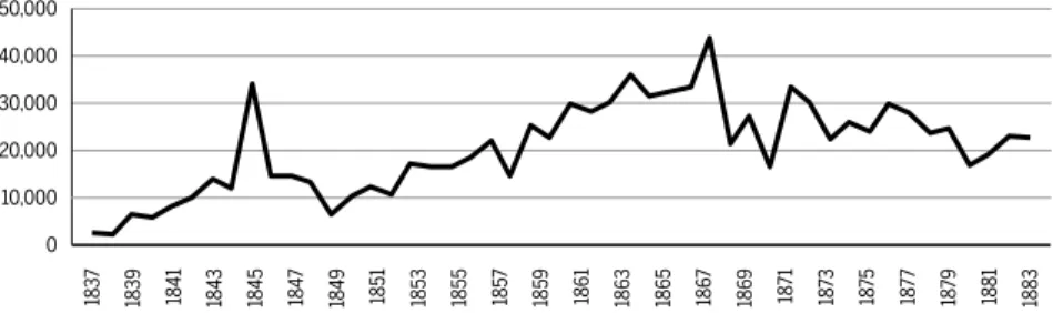
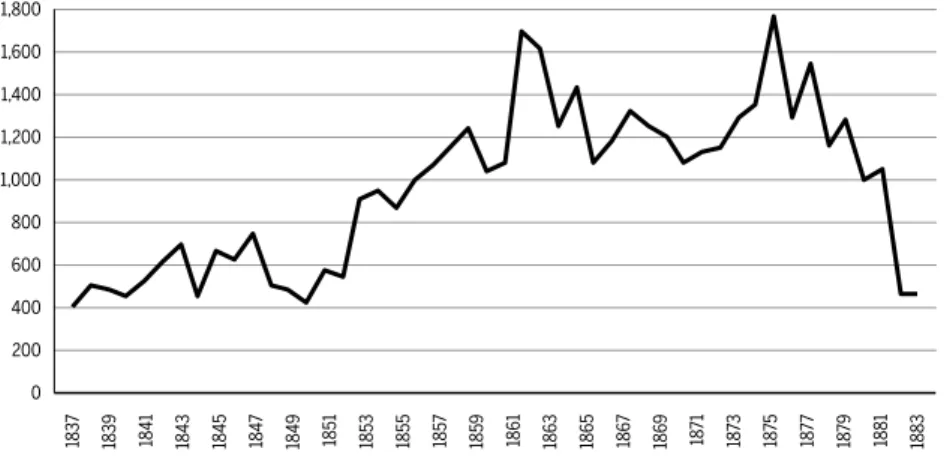
Figure 1 shows the beneficial impact of the Imperial government’s policies surrounding beef jerky production in Rio Grande do Sul, which resulted in a steady increase in exports after 1851. Until the end of the Paraguayan War in March 1870, the Brazilian beef jerky industry benefited from its protectionist advantage over Uruguayan production. It is impor-tant to note that, according to the Province’s President Israel Rodrigues Barcellos, the sharp drop in exports shown in 1869 was due to heavy rains that destroyed major roads leading to slaughterhouses (Provincial Presi-dential Report, 1869, p.5). Since beef jerky production sites were located in cities near the east coast, such as Pelotas, and cattle were raised in cit-ies at the border of Uruguay, a disruption on the roads could paralyze production. Also, in 1870, pastures in Rio Grande do Sul were ravaged by a foreign herb (epazote) that had already caused damage in Uruguay and Argentina (Diário do Rio de Janeiro, 1870, ed. 167, p.2). The beef jerky export data shows that the industry’s stagnation began after 1870. In 1872, the Rio Grande Business Association financed some studies to understand the problems facing the industry (Cardoso, 2003, p.214). Again, taxes were to blame for the lack of competitiveness.
Figure 1 Rio Grande do Sul beef jerky exports (tons)
Source: FEE (2004)
Even in the 1860s, however, a decade with increasing growth in exports, Rio Grande do Sul production lagged behind when compared to Uruguay.
50,000
40,000
30,000
20,000
10,000
0
183
7
1839 1841 1843 1845 184
7
1849 1851 1853 1855 185
7
185
9
1861 1863 1865 186
7
186
9
18
71
18
73
18
75
18
77
18
79
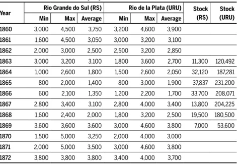
According to a commercial Rio de Janeiro newspaper, there was some con-cern in 1865 regarding the quality of Rio Grande do Sul beef jerky. People preferred the Rio de la Plata product, and it had “taken over the markets of Rio de Janeiro” (Diário do Rio de Janeiro, 1865, ed.8, p.3). Brazilian beef jerky still had a better market share in Bahia, but the newspaper article stated that it was facing increasing competition from Uruguay there as well. Data from Rio de Janeiro newspapers show that despite similar pri-ces, Uruguay’s beef jerky already dominated the most important Brazilian market by the 1860s. Table 2 presents data with prices (réis) and beef jerky stocks (arrobas) from newspapers for the first week of each year presented. This data should not be interpreted as an average price for the whole year, but it gives information about differences in prices from both regions. Using data from the beginning of each year also makes it possible to com-pare the stocks available for each product at the end of the previous year.
Table 2 Prices and stocks of beef jerky in Rio de Janeiro
Year Rio Grande do Sul (RS) Rio de la Plata (URU) Stock (RS)
Stock (URU) Min Max Average Min Max Average
1860 3,000 4,500 3,750 3,200 4,600 3,900
1861 1,600 4,500 3,050 3,000 3,200 3,100
1862 2,000 3,000 2,500 2,500 3,200 2,850
1863 3,000 3,200 3,100 1,800 3,600 2,700 11,300 120,492
1864 1,000 2,600 1,800 1,500 2,600 2,050 32,120 187,281
1865 800 2,000 1,400 800 3,000 1,900 37,837 231,200
1866 600 2,100 1,350 1,200 2,200 1,700 33,700 208,071
1867 2,800 3,400 3,100 2,800 4,000 3,400 13,800 204,225
1868 1,600 2,400 2,000 1,800 3,200 2,500 19,500 180,500
1869 3,600 3,600 3,600 3,000 4,600 3,800 7,000 53,600
1870 1,500 5,000 3,250 2,000 4,000 3,000
1871 2,000 5,000 3,500 3,000 4,600 3,800
1872 3,800 3,800 3,800 3,400 4,000 3,700
Source: Diário do Rio de Janeiro – Biblioteca Nacional Digital (Several Years)
approxi-mately 45 percent in coffee plantation areas between 1872 and 1887 (Luna; Klein, 2010, p.320). Further, the immigrants who replaced slave labor did not consume dried meat (Holloway, 1980). Following the 1888 abolition of slavery in Brazil, beef jerky production continued its slow decay. Yet, at the beginning of the twentieth century, the sector remained relevant at the regional level. In 1909, Álvaro Baptista, Finance Minister of Rio Grande do Sul, deplored the inability of the region to move away from an industry that would inevitably disappear (Fonseca, 1983).
3
Meat exports in Uruguay
The political and economic disorganization of Uruguay, which resulted from constant wars and bad commercial treaties, came to a halt in 1856 (Rock, 2000). From that period until 1865, Blanco’s and Colorado’s head politicians tried to come together in order to create a national awareness and condemn the country’s past submission to foreign countries (Casal, 2004). However, with or without political conflicts, Uruguay’s economy was heavily reliant on international trade (Barran; Nahum, 1984). Unlike Rio Grande do Sul, which had a large market in other Brazilian provinces, Uruguay depended on foreign markets.
After 1860, due to the 1851 treaty and changes in global demand, the beef jerky industry started losing its relevance in Uruguayan exports. Also, as a consequence of the United States Civil War (1861–1865), Uruguayan exporters had the opportunity to diversify by increasing wool production, since the country was one of few regions in the world where bovine and ovine cattle shared the same territory. The United States was the main cot-ton supplier to Europe’s textile industry, and it faced an abrupt decline in production during the war years. This slowdown heightened the demand for cotton from other regions, and it also allowed for cotton substitutes, such as wool, to enter the market (Barran; Nahum, 1967; 1984).
Within a decade (1860–1870), the wool industry established itself as one of the major economic sectors in Uruguay, enabling the rise of medi-um-sized estancieiros and making ovines more sought after among cattle raisers. Cattle diversification, however, did not happen for the Brazilian
in Brazil continued their extensive breeding programs that were geared toward the beef jerky industry in Rio Grande do Sul. The favorable eco-nomic scenario in Uruguay resulting from wool exports lasted until the
end of the North American conflict. At this point markets normalized once again, and the United States instituted the Morrill Tariff, a protection against foreign wool. Thus, the Uruguayan wool sector lost a great deal of its market. According to a contemporary writer, in the 1870s higher land prices and labor wages represented the end of easy money for sheep farm-ers (Burton, 1870, p.88).
Uruguay’s prosperous years led to the perception in the literature that, beginning in 1860, estancias acquired a modern vision, with innovative technologies coming from social groups with a “clear capitalist project” (Minello, 1977, p.578). Nevertheless, that capitalist project seems to have come from a greater availability of resources from the 1860s economic boom, as the increased need for leather and wool offered incentives to invest in steam machinery that would draw out animal grease and im-prove productivity.
An example of the shift in market demand came in 1862 with the first meat extract factory in the Prata region, established by a Belgian com-pany. Located in the city of Fray Bentos, in a place previously used as a slaughterhouse (or saladero), the factory was sold to a British company in 1866, giving birth to the Liebig’s Extract of Meat Company. Anglo-Irish traveler Thomas J. Hutchinson visited the factory in 1867, and his first im-pression was that Liebig’s was unlike other saladeros that he had seen; he stated: “The general atmosphere, about the engine-house particularly, be-ing suggestive of rich beef-gravy” (Hutchinson, 1868, p.411). Hutchinson reported that each animal produced ten pounds (4.5kg) of meat extract and that the factory had the capacity to produce 250 pounds (114kg) per day. Nonetheless, this level of production still did not meet European demand, which was four times greater (Hutchinson, 1868, p.412).
hour, and “nothing was wasted”. Gallenga’s estimates of Liebig’s revenue revealed that the company had annual profits of £81,000, and it used 6,000 tons of coal and around 128,000 pounds of salt (Gallenga, 1881, p.300). Like Hutchinson, Gallenga also noticed the cleanness of Liebig’s in com-parison to other saladeros. The Italian described one instance of visiting a regular saladero, in which the host family gave him a tour. He explained that no one seemed bothered by the amount of blood and animal remains in the area; following the visit, he detailed, “We went back to the break-fast-room, the dwelling-house being so close to the saladero that the flies would not have allowed us to eat in peace for one moment” (Gallenga, 1880, p.301).
The information about infrastructural differences between Liebig’s and regular saladeros shows the importance of meat extract to Uruguay’s exports.This extract had higher added value than beef jerky and could be easily shipped to distant markets. Further, this situation created incen-tives to increase export diversification, reducing the market importance for beef jerky.3
The increase in export diversification was also reinforced by another regional conflict. Even with the favorable economic conditions and no po-litical conflicts after the pact between the Blancos and Colorados in 1856, confrontation between the parties resurfaced as a result of geopolitical tension in the years leading up to the Paraguayan War. Once more Brazil interfered giving support to Colorado’s party president Venancio Flores against the Blanco party, which had the support of the Paraguayan Mar-shal Solano López. One reason for Brazil’s intervention was the constant territorial disputes in a region that housed several Brazilian cattle ranchers (Moraes, 2008).4 With Argentina and Paraguay supporting different par-ties, Brazil had to make a statement and sent in terrestrial forces com-manded by the Baron of Tamandaré (Casal, 2004).
Brazil used border areas as a base for war operations and its monthly subsidy to its Oriental Division caused a rapid economic expansion in
3 Nevertheless, meat extract still did not have the same appeal as fresh meat: “[…] except for the war years, when a large demand for this kind of meat (canned and tasajo) for the armies existed, the exports have been small. The canning plants must give way, as the cattle industry improves, to the modern packing plants which turn out the higher grades of meat” (Jones, 1927, p.366).
Uruguay from 1865 to 1868: “The incoming gold allowed Montevideo entrepreneurs to establish new navigation, railroad, telegraph, and build-ing companies as well as new steam factories, new banks, credit brokers, and even mining operations” (Casal, 2004, p.137). The artificial growth increased livestock and meat extract sales, causing land and cattle prices to rise. The high profit rates led banks to increase credit lines, making invest-ments possible on the first meat refrigerated storages. Growth came to a sudden halt only in 1868, when the inflow of Brazilian gold ended as the war drew to a close (Casal, 2004).
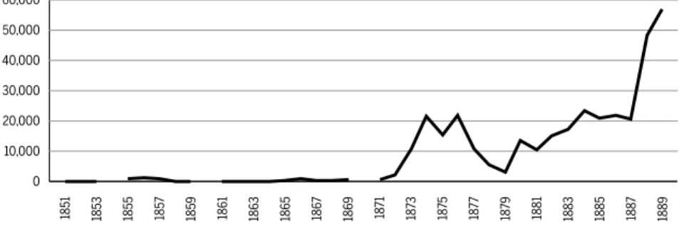
Despite the increase in production during the Paraguayan War, Uru-guay did not increase its bovine meat supply to external markets because low-quality meat had only limited demand internationally. European con-sumers, especially the British, rejected beef jerky (Minello, 1977, p. 580). Seen as food for slaves in Brazil and Cuba, accounts report that “its ap-pearance to Europeans [was] absolutely offensive” (Newcastle Courant, Sep, 1866, p.3). According to contemporaneous newspapers:
Some five hundred or six hundred different experiments have been made to cure South American beef so as to make it a marketable article in Europe; but no real success has as yet attended the efforts. The meat [charque] as forwarded has been refused by the working classes in England, and rejected by the French navy (Dublin Evening Mail, Jun, 1869).
Figure 2 Uruguay’s exports of preserved meat otherwise than by salting, 1850-1889 (cwt)
Source: Ledgers of Imports under Countries (CUST 4), British National Archives.
The increase in demand for non-salted meat in Europe did not affect only the Plata region. By the end of the 1860s, refrigerated meat was shipped across the United States and had begun to reach European markets (Tim-mons, 2005; Wade, 2003). Indeed, the business of hermetically sealed
pac-king for meats and vegetables was flourishing in states like Maine (Bath Chronicle and Weekly Gazette, Sep, 1866). The increase in North American production, achieved through a series of labor-saving devices, sought to take advantage of all cattle parts. The “jerked beef” produced in Chicago was sold to impoverished workers in the West Indies, and it was made of parts that had been previously disposed, such as necks and shanks (Wade, 2003, p.8). Likewise, Uruguay managed to increase its exports of low-qua-lity meat after the 1870s to Brazil partially by the increase in production of better quality meat for European markets.5 According to Millot and
Ber-tino (1996, p.169), Uruguay’s beef jerky industry peaked in 1863, when other industries involving cattle began to rise.
Bovine livestock increased in Uruguay between 1852 and 1900 from 1,800,000 to 6,800,000, whereas the growth in sheep was from 796,000 to 18,608,000 (Jones, 1927). While these figures highlight the difference in growth between bovine and ovine cattle, it should be noted that the figures for 1852 represent a low point in the number of livestock, given this was the period of the Guerra Grande. The main point is that the pro-duction of low quality meat decreased throughout the years. From 1921 to 1923, for example, beef jerky represented only five percent of the
Uru-5 According to Hutchinson (1868), “Only in Brazil and Cuba, where it is bought on account of its cheapness to feed the slaves, has this charqui ever been a marketable article.”
60,000
50,000
40,000
30,000
20,000
10,000
0
1851 1853 1855 185
7
185
9
1861 1863 1865 186
7
186
9
18
71
18
73
18
75
18
77
18
79
1881 1883 1885 188
7
188
guay’s commodity exports (Jones, 1927). Meanwhile, for Rio Grande do Sul, the average production of low-quality meat was 20.8 percent (FEE, 2004). Higher quality meat, such as refrigerated (7 percent), frozen (14 per-cent), and canned (7 perper-cent), left beef jerky behind as a displaced product in the Uruguayan Republic (Finch, 2005). On the other hand, Rio Grande do Sul exported only 0.33 percent of canned meat and 5.33 percent of packed meat. Economic backwardness can be verified by comparing the dates in which packinghouses were established in both regions: Frigorifica Uruguai, in 1905, and the first in Rio Grande do Sul, in 1918 (Jones, 1927).
4
Interpretations for the Brazilian industry’s decline
Despite differences in fiscal incentives and access to foreign capital between Rio Grande do Sul and Uruguay, characterization of slave labor as “noneconomic” remains an important explanation for why Rio Gran-de do Sul could not compete with Uruguay, which increasingly used free labor after the 1840s (Borucki et al, 2004). The use of a less productive la-bor force, the “irrationality hypothesis”, was defended by several authors, such as Corsetti (1983), Cardoso (2003), and Pesavento (1980). Authors such as Décio Freitas (1980, p.35) argued that nothing could be more “anti--economic” than slave labor. There are two common reasons for this kind of argument: the notion that restricted labor division resulted in lower pro-ductivity; and the idea that the constant vigilance necessary when using slave labor was more expensive than employing free workers. Also, flexi-bility in wage labor markets allowed for the reduction of workers during economic slowdowns (Cardoso, 2003).
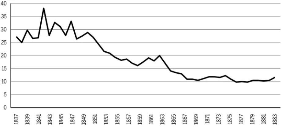
Costs became increasingly important after the 1860s when, according to Pesavento (1980), the saladero platino began to modernize its industry.6 Rising slave prices after the end of slave trade in 1850 represented an important increase in costs for Brazilian production. Figure 3 shows the prices for male slaves, between 20 and 29 years old, who worked with beef jerky production in Rio Grande do Sul. With the sudden stop in labor supply, European immigration policies became one of the main concerns for Brazilian politicians (Carvalho, 2010; Skidmore, 1974). Contemporary
authors, such as the Italian researcher G. B. Marchesini, stated that the “re-cent experience” with foreign labor in Brazil made it clear that “free labor [was] more productive in any culture” (Marchesini, 1877, p.76).7
Figure 3 Average male slave prices (mil-reis)
Source: State of Rio Grande do Sul Archive.
The view of slave labor as less productive than free labor remained practi-cally uncontested until the work of Conrad and Meyers (1958). Afterwards, Fogel and Engerman (1989) also provided evidence that captive labor had been even more productive than wage labor in some circumstances, and that the reason for slave use in the United States southern plantations was economic, not only cultural. For Brazil, Mello (1978) and Versiani (1994) also raised questions about captive labor economic inferiority despite the absence of data to compare all labor costs related to free labor, which was mainly represented by immigrants. By the end of the 1870s, Rio Grande do Sul already had a strong presence of foreigners, not only at agricultural colonies but also in urban areas (Trento, 1989). Nevertheless, the only con-nection they had with the beef jerky industry was through the production and selling of hides to external markets.8 Enslaved people were still largely
7 Many contemporary Brazilian authors and politicians quoted European authors like Adam Smith on the benefits of free labor: “The experience of all ages and nations, I believe, demon-strates that the work done by slaves, though it appears to cost only their maintenance, is in the end the dearest of any. A person who can acquire no property, can have no other interest but to eat as much, and to labour as little as possible” (Smith, [1776] 2007, p.252).
8 Quadro Estatístico e Geográfico da Província de S. Pedro do Rio Grande do Sul, p.81, 1868.
1,000
800
600
400
200
0 1,800
1,600
1,400
1,200
183
7
1839 1841 1843 1845 184
7
1849 1851 1853 1855 185
7
185
9
1861 1863 1865 186
7
186
9
18
71
18
73
18
75
18
77
18
79
used in the most prosperous economic regions of Rio Grande do Sul and, as Cardoso explained, “The charqueadores, who were supposed to be the more ardent defenders of abolition, remained proslavery until the end” (Cardoso, 2003, p.257).
Monasterio (2003; 2005) also provides evidence that slave use at the charqueadas was rational and operated at a lower cost than free labor. He makes reference to the unsuccessful attempts to introduce the “platine system” in Rio Grande do Sul. During the Paraguayan War, there are re-cords of attempts to send prisoners and Paraguayan children to work at the saladeros, to lower industry wages (Casal, 2004, p.131-35). Another reason for the high costs of wages in Uruguay’s saladeros had to do with the end of the Commerce Treaty with Brazil in 1861, due to protests of unfair competition by President Bernardo Berro. The president prohibited long-term work contracts between Brazilians and “citizens of color” due to the possibility of using slaves, who “represented half of the wages from a Uruguayan rural worker” (Souza; Prado, 2002, p.16).
Another potential cost for those involved with the charque industry was the possibility of revolts and runaways. Indeed, production sites and the cattle-herding region (campanha) were near the Uruguayan border, where slavery was illegal. This proximity led authors like Luiz Targa and Décio Freitas to assert that slave use was not possible in the cattle-herding re-gion (Nogueról et al, 2007, p.13). Versiani (1994), however, showed that slaves responded to a series of positive incentives that owners used to increase productivity and prevent runaways in frontier regions. Nogueról et al (2007) also presents evidence that slaves used horses in the open fields of Rio Grande do Sul on a regular basis, and some were even horse tamers. One of the negative incentives for runaways was Uruguay’s responsibil-ity, under the 1851 treaty, to return any black individual suspect of being a runaway slave. In addition, a large part of the Uruguayan border was controlled by Brazilian ranchers (Souza, 2002, p.13).
Rio Grande do Sul.9 The new database used in this paper also provides evidence that, between 1850 and 1884, there was significant labor special-ization at the charqueadas. From the 637 male and healthy slaves’ sample, half of them (319) had declared an occupation. Also, data from the 1865 inventory of businessman José Inácio da Cunha shows that his 115 slaves had seventeen different occupations at his charqueada.10 Women were also divided according to occupations; they worked as cooks, farmhands, laun-dresses, and seamstresses, among other jobs.
Division of labor also occurred within the production line itself; some slaves killed the herds, others cleaned the animals, and others salted the meat. These point to a division of labor that was similar to the free la-bor system. Nogueról et al (2002; 2007) noticed that, after 1850, slaves with declared occupations at post-mortem inventories had selling prices 15 per cent higher on average.There was a perception by slave owners of productivity differentials among captives. Brazilian historiography also provides ample evidence that slave labor specialization included even complex tasks, which demanded special training (Schwartz, 1988; Luna, Klein, 2010).
Another recent hypothesis concerning the Brazilian beef jerky indus-try’s decline comes from Monasterio (2005). He raises the possibility of a “Dutch disease” phenomenon, where a boom in the export sector affects other sectors subject to international competition. In the charqueadas’ case, the expansion of coffee production drove demand for non-tradable prod-ucts, which increased their prices. Along these lines, the reduction in the competitiveness of Brazilian beef jerky would have occurred through the appreciation of the real exchange rate. Figure 4, which presents a real ex-change rate series for Brazil, provides evidence that there was a currency appreciation after 1850, when coffee exports began to grow at a faster rate.
Comparing the literature for Brazil and Uruguay, it is interesting to note that the beef jerky industry’s decline after 1870 occurred in both countries, as Finch (2005) and Millot and Bertino (1996) argued for Uruguay. Uru-guayan historiography even raises the possibility of a “resource curse” due to its inability to compete in the meat market with countries with similar
9 The cities were Dom Pedrito, Encruzilhada and Rio Pardo.
characteristics, such as New Zealand.11 Such concern existed despite the fact that New Zealand surpassed Uruguay’s cattle raising only in the twentieth century. According to authors who support this hypothesis, the good pastures from the Pampas promoted inertia. With less risk, investments made in Uruguayan cattle received smaller profits, but they kept the industry operating (Barrán; Nahum, 1984, p.670). Recent research confirms that land productivity was higher in Uru-guay than in New Zealand in the nineteenth century (Alvarez, 2014; 2015).
Figure 4 Real exchange rate (index)
Source: Moura Filho (2006); Twigger (1999); Lobo (1971)
Differences in land productivity can be an important factor to explain why Rio Grande do Sul was unable to change its production to meet the gro-wing demand of non-dried meat from abroad during the first globaliza-tion. Recent research emphasizes that the south-west region of Uruguay was more suitable for livestock production than the region that borders Brazil (Bertino et al, 2005; Moraes, 2008). This could partially explain why British capital did not invest in Rio Grande do Sul, providing the resources needed to modernize the industry.12 This hypothesis, however, is beyond the scope of this work because the necessary micro-data to estimate pro-ductivity differences is not available.
11 According to Barrán and Nahum the British colonists were forced to respond to the chal-lenge presented by the rugged and wooded territory of New Zealand. From the start, in the first half of the nineteenth century, they sowed pastureland. Uruguay, as has already been stated, had the diabolical blessing of ease. Its natural pastures did not necessitate the inven-tion of the soil; it was already there (1984, p.670).
12 I thank the anonymous referee that pointed out this factor.
25
20
15
10
5
0 40
35
30
183
7
1839 1841 1843 1845 184
7
1849 1851 1853 1855 185
7
185
9
1861 1863 1865 186
7
186
9
18
71
18
73
18
75
18
77
18
79
Therefore, on the next section, we provide quantitative analysis on the two hypothesis raised by previous literature for the industry of Rio Grande do Sul. Analyzing the impact of the exchange rate and labor costs on prices and quantities exported can contribute to the debate by changing the variables of interest for future research. The quantities ex-ported, shown in Figure 1, present evidence that exports did not decline, but instead stagnated after 1870 following an early period of high pro-tection. The industry’s decline at the beginning of the twentieth century can only be understood in the context of the abolition of slavery, which eliminated the main consumers of beef jerky. After the abolition, only a fraction of the poorest members of the population continued to consume salted, dried meat.
5
Labor markets or Dutch disease?
In this section we test the different hypotheses that were previously pre-sented, in order to determine the causes of the beef jerky industry’s decli-ne. The sample begins in 1837, right before the beginning of the Farrou-pilha Civil War, and it goes until the de facto 1884 abolition of slavery in Rio Grande do Sul. The variables used are: quantities (in tons) and prices (in mil-réis) of beef jerky exported (FEE, 2004), slave prices, real exchange rate and salt prices (IPEA).The inclusion of salt prices is significant due to the debate, at the beginning of the 1850s, surrounding the possibility that taxes on salt would make local production uncompetitive.
For the labor market hypothesis, we built a series of slave prices for the three main cities associated with beef jerky production: Pelotas, with 1,463 observations, Rio Grande, with 751, and Porto Alegre, with 1,289. These observations refer to slaves registers from postmortem inventories between 1830 and 1884. From this data, we selected only healthy males, between 20 and 29 years old, who represented the most valued and pro-ductive labor for the industry and account for the highest slave prices.13 We adjusted these prices using the Feinstein (1995) consumer price index in silver prices. The usual Brazilian price index for the period analyzed is Lobo (1971), which is based on a limited basket of consumer goods in Rio
de Janeiro. Since slaves represented a significant investment during the period under analysis, using Lobo’s price index would distort the series due to higher fluctuation from non-durable consumer goods. Lobo’s index, with the 1919 weighting, was used to deflate the price of beef jerky and salt.Concerning the Dutch disease hypothesis, a real exchange rate series, presented in Figure 3, was built using data from the nominal exchange rate by Moura Filho (2006), together with the price level for England from Twigger (1999), and the domestic price level of Lobo (1971), which con-tains beef jerky prices.
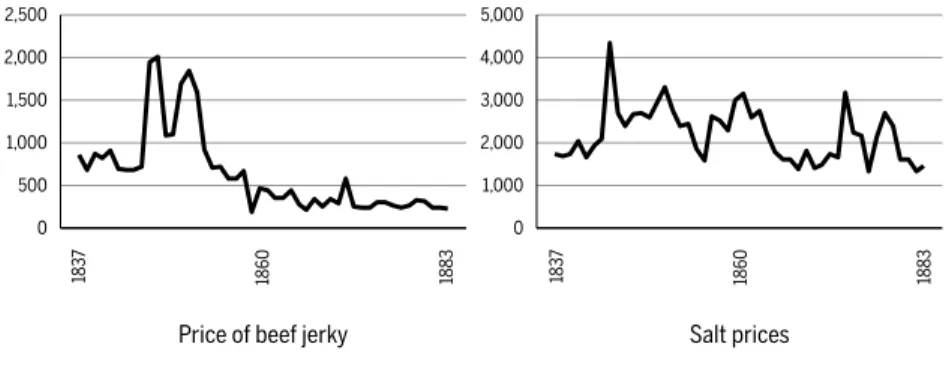
Two other series were tested in the empirical analysis, but they were discarded. The first one is Bértola’s (1998) estimations of the cattle in-dustry in Uruguay. The problem is that this data set begins in 1870, at the latter half of the present analysis. The other difficulty is that the estimations do not relate solely to beef jerky production, due to the fact that Uruguay diversified its exports, moving away from beef jerky after 1870. The other series tested measures Brazilian coffee exports, since this industry housed the labor force that served as the main consumers for beef jerky. The reason why this variable was excluded is that it is highly correlated with the real exchange rate. Also, since annual data is used, the limited number of observations requires certain restrictions in the number of parameters that can be estimated. Other information that should be noted comes from Figure 5. As previously stated, both beef jerky and salt prices were deflated using Lobo’s price index, however, as the real exchange rate graph shows, the price index probably distorts the real prices before 1855.
Figure 5 Beef jerky and salt prices (mil-réis)
Source: FEE (2004), IPEADATA (2014). 2,500
2,000
1,500
1,000
500
0
5,000
4,000
3,000
2,000
1,000
0
Price of beef jerky Salt prices
183
7
1860 1883 183
7
In order to analyze the relationship between variables, it was first neces-sary to verify if the series are stationary. The appendix presents the results for the unit root tests, which show that all variables, except salt prices, are integrated of order 1. Since this study’s intention is to analyze long-term processes and not their rates of change, a Vector Error Correction model (VECM) is used to accommodate the nonstationary features of the data. To test for the existence of a long-run equilibrium relation between the va-riables, the Appendix presents a cointegration analysis using the Johansen procedure. Given that the series has strong fluctuations in some specific periods, all variables were transformed to their logarithmic form to mini-mize heteroskedasticity issues (Banerjee et al, 2003).
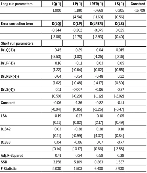
Using the Johansen procedure, both Maximum Eigenvalue and Trace statistics indicate the existence of one cointegration vector for the loga-rithm of Beef Jerky Exports (LQ), Prices (LP), Slave Prices (LS) and real exchange rate (LRER). Since Salt Prices (LSA) is stationary, this variable is incorporated as exogenous in the VECM. In addition, two exogenous year dummies were used. One dummy appears in 1883 (d1883), and is related to the plunge in prices in anticipation of the end of slavery in Rio Grande do Sul. The other appears for the year 1842 (d1842), for the real exchange rate series. Also, to comply with the assumptions of the model, the appen-dix presents statistics for the LM autocorrelation test and normality tests for the VECM residuals. Table 3 presents the results for the cointegration vectors and their adjustment coefficients.
Since the VECM relates to simultaneous representations of a system, its individual coefficients do not have a clear interpretation. Our primary interest rests on the error correction terms, which show if variables adjust in the short run to deviations from equilibrium. Based on the results from Table 3, the only variable that does not adjust is Slave Prices. The error cor-rection term equal to zero means that this variable is weakly exogenous (Burke, Hunter, 2005). Also, the long-run parameter of the real exchange rate is not different from zero, meaning that this variable is exogenous in the long term.
In the results, the error correction parameters must be consistent with the proposed model. From the three variables that have an error correction term, the Real Exchange Rate does not correct short term deviations.14 The
low coefficient (-0.07) shows that this variable acts in a very weak manner against adjustment. As expected, quantities and prices are responsible for the adjustment to deviations from equilibrium. In order to better under-stand the relations between the variables, Table 4 shows the results from variance decomposition analysis for five periods. From the result, there is no evidence that changes in slave prices had a significant impact on the quantities and prices of beef jerky exports. For the real exchange rate, there is some small impact on the quantities exported.
Table 3 Vector error correction estimates
Long run parameters LQ(-1) LP(-1) LRER(-1) LS(-1) Constant
1.000 1.190 -0.668 0.205 -16.709 [4.54] [-1.60] [0.56]
Error correction term D(LQ) D(LP) D(LRER) D(LS)
-0.344 -0.202 -0.075 0.025 [-3.86] [-1.78] [-2.93] [0.40]
Short run parameters
D(LQ(-1)) -0.45 0.29 -0.04 0.015
[-3.53] [1.82] [-1.25] [0.16]
D(LP(-1)) 0.16 -0.11 0.03 0.05
[1.22] [-0.64] [0.82] [0.55]
D(LRER(-1)) 0.64 -0.24 -0.48 0.22
[1.62] [-0.48] [-4.17] [0.80]
D(LS(-1)) 0.11 -0.007 -0.06 -0.27
[0.59] [-0.29] [-1.12] [-2.02]
Constant -0.06 -1.36 -0.82 -0.41
[-0.04] [0.85] [-2.26] [-0.47]
LSA 0.19 0.17 0.10 0.05
[0.11] [0.82] [2.17] [0.49]
D1842 0.03 -0.38 0.38 0.18
[0.11] [-0.99] [4.32] [0.84]
D1883 0.04 -0.06 0.07 -0.77
[0.14] [-0.17] [0.86] [-3.58]
Adj, R-Squared 0.41 0.24 0.58 0.38
SSR 3.158 5.109 0.263 1.537
F-Statistic 5.030 1.503 6.430 2.938
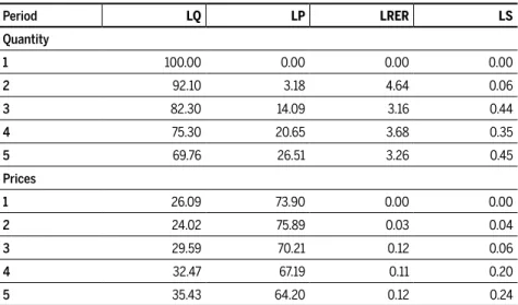
Table 4 Variance decomposition of quantity and prices of beef jerky exported
Period LQ LP LRER LS
Quantity
1 100.00 0.00 0.00 0.00
2 92.10 3.18 4.64 0.06
3 82.30 14.09 3.16 0.44
4 75.30 20.65 3.68 0.35
5 69.76 26.51 3.26 0.45
Prices
1 26.09 73.90 0.00 0.00
2 24.02 75.89 0.03 0.04
3 29.59 70.21 0.12 0.06
4 32.47 67.19 0.11 0.20
5 35.43 64.20 0.12 0.24
As the interest relies on the impact of shocks in the real exchange rate and slave prices in beef jerky production, in order to complement the previous table, Figure 6 presents results of an Impulse Response Analysis for ten periods. Since slave prices do not have any impact (less than 0.3 percent) on quantity exported and price, we only present the graph for the real exchange rate in Figure 6.
Figure 6 Impulse response analysis of LQ to LRER
The quantitative analysis presented in this section provides no evidence that the rise in slave prices had a negative impact on beef jerky produc-tion. There was some impact from the exchange rate on the quantity of exports, but its effect is small and cannot be considered as an important factor for production stagnation in Rio Grande do Sul.
2 1 0 -1 -2
6
Conclusion
Beef jerky’s production decline was not restricted to Brazil; rather, it was a global phenomenon. The end of slavery in several countries across the Americas during the second half of the nineteenth century, as well as an increase in wages in Europe’s consumer markets, led to the demand for better quality products.Tariff protection and political instabilities in Uru-guay benefited Rio Grande do Sul beef jerky production until the end of the 1860s, when demand for higher-quality meat forced the industry’s market share to decrease. We provide evidence that differences in labor regimes did not account for the different trajectories in livestock industries between Rio Grande do Sul and Uruguay. We also found that, despite some impact fromthe real exchange rate on prices, the effect was too small to account for the sector’s decline. With the new series on Rio de Janeiro market prices, we are able to conclude that both products had similar pri-ces, and different market shares were related to product quality and higher productivity in Uruguay.
Further, since wage labor was more expensive, Uruguay had incentives to use more capital-intensive production because its labor costs were high-er than in Brazil’s.Thhigh-erefore, the growth of Uruguay’s cattle industry arose out of the diversification of its exports, especially canned and refrigerated meat.Foreign investment from British companies, which made the Uru-guayan transition possible, was absent across the border. This indicates that the increase in beef jerky productivity in Uruguay was probably an indirect effect of higher demand in non-salted meat. As was the case in the United States, higher demand in non-salted preserved meat led to an increase in cattle stock, with the inferior parts of the cattle used to produce beef jerky.
In other words, international demand, represented by European mar-kets, had changed; and Uruguay managed to transform and diversify its industry to meet consumers’ needs. Even though it could not compete with the United States’ meatpacking industry, the Rio da Prata region made sub-stantial improvements in the last quarter of the nineteenth century. At the same time, the Rio Grande do Sul industry stagnated; beef jerky remained crucial to the province, but was no longer in high demand in other regions.
the way Uruguay did. Nevertheless, the evidence presented contributes to the literature by using new quantitative data to test previous hypotheses. Additional research is necessary to analyze the impact of potential differ-ences in land productivity between the regions.
References
Primary Sources:
Inventories from the Rio Grande do Sul Public Archive.
Quadro Estatístico e Geográfico da Província de S. Pedro do Rio Grande do Sul, 1868. Available at the archive of Fundação de Economia e Estatística do Rio Grande do Sul.
Provincial Presidential Reports (1830-1930). Center for Research Libraries – Global Resources Network. Available at http://www-apps.crl.edu/brazil/provincial.
From the Biblioteca Nacional Digital Newspaper Archive: O Rio-Grandense, 1851.
Correio Mercantil, e Instructivo, Político, Universal, 1851a ed 1. Correio Mercantil, e Instructivo, Político, Universal, 1851b ed 4. Diário do Rio de Janeiro, 1860-1872.
Ledgers of Imports under Countries (CUST 4), British National Archives. From the British Newspaper Archive:
Bath Chronicle and Weekly Gazette - Thursday 13 September 1866. Newcastle Courant, Friday, September 14, 1866 p.3.
Dublin Evening Mail - Saturday 26 June 1869.
Secondary Sources:
ÁLVAREZ, Jorge. Instituciones, cambio tecnológico y productividad en los sistemas agrarios de Nueva Zelanda y Uruguay. Patrones y trayectorias de largo plazo (1870-2010). Thesis for doctorate in economic history. Faculty of Social Sciences, University of the Republic, Uruguay, 2014 ÁLVAREZ, Jorge. Technological change and productivity growth in the agrarian systems of New
Zea-land and Uruguay (1870-2010). Workshop on Comparative studies of the Southern Hemi-sphere in global economic history and development. Research Institute for Development, Growth and Economics (RIDGE), Montevideo 27-29 March, 2015.
BANERJEE, Anindya; DOLADO, Juan; GALBRAITH, John; HENDRY, David. Co-Integration, Error-Correction, and the Econometric Analysis of Non-Stationary Data. New York: Oxford Uni-versity Press, 2003.
BELL, Stephen. Campanha Gaúcha: A Brazilian Ranching System, 1850 – 1920. Stanford: Stanford University Press, 1998.
BERTINO, M; BERTONI, R.; TAJAM, H. Historia Económica Del Uruguay. Tomo III: La econo-mia del batllismo y de los años veinte. Montevideo: Ed. Fin de Siglo, 2005.
BÉRTOLA, Luis. El PBI Uruguayo 1870-1936 y otras estimaciones. FCS-CSIC, Montevideo, 1998. BETHELL, Leslie. The Abolition of the Brazilian Slave Trade. Britain Brazil and the Slave Trade
Question 1807-1869. Cambridge: Cambridge University Press, 1970.
BORUCKI, Alex; CHAGAS, Karla; STALLA, Natalia. Esclavitud y Trabajo. Unestudio sobre los afrodescendientes en la frontera uruguaya 1835-1855. Montevideo: Ed. Pulmón, 2004. BURKE, Simon; HUNTER, John. ModellingNon-Stationary Time Series. A Multivariate
Ap-proach. Hampshire: Palgrave Macmillan, 2005.
BURTON, Captain Richard F. Letters from the Battle-fields of Paraguay. London: Tinsley Broth-ers. Acervo da Brasiliana Digital USP, 1870.
CARDOSO, Fernando Henrique. Capitalismo e Escravidão no Brasil Meridional. Rio de Janeiro: Civilização Brasileira, 2003.
CARVALHO, José Murilo de. Teatro das Sombras. A Política Imperial. Rio de Janeiro: Civiliza-ção Brasileira, 2010.
CASAL, Juan Manuel. Uruguay and the Paraguayan War. In: KRAAY, H.;WHIGHAM, T. L.I Die with My Country. Perspectives on the Paraguayan War, 1864–1870. University of Ne-braska Press, 2004.
CONRAD, Alfred. H.; MEYER, John R. The Economics of Slavery in the Antebellum South. The Journal of Political Economy, 26 (2), pp. 95-130, 1958.
CORSETTI, Berenice. Estudo da charqueada escravista gaúcha no século XIX. Dissertação (Mes-trado em História) – Departamento de História, UFF, Niterói, 1983.
FARINATTI, Luís Augusto. Os grandes estancieiros e além: criadores de gado na fronteira meridional do Brasil (Alegrete, 1831-1970). História Econômica & História de Empresas, XI. 1, pp. 91-117, 2008.
FEE. As Relações de Comércio do Rio Grande do Sul – do século XIX a 1930. Porto Alegre, Outu-bro, 2004.
FEINSTEIN, Charles. Changes in Nominal Wages, the Cost of Living, and Real Wages in the United Kingdom over Two Centuries, 1780–1990. In: SCHOLLIERS, P.;ZAMAGNI, V. (Eds.). Labour’s Reward. Aldershot, Hants: Edward Elgar. p. 3–36, 258–266, 1995.
FINCH, Henry. La economía política del Uruguay contemporáneo,1870-2000. Montevideo: Edicio-nes de la Banda Oriental, 2005.
FOGEL, Robert; ENGERMAN, Stanley. Time on the Cross. The Economics of American Negro Slavery. Nova York: Norton, 1989.
FONSECA, Pedro. RS: Economia e Conflitos Políticos na República Velha. Porto Alegre: Mercado Aberto, 1983.
GALLENGA, Antonio. South America. London: Chapman and Hall. Acervo da Brasiliana Digi-tal USP, 1881.
HOLLOWAY, Thomas. Immigrants on the Land. The University of North Carolina Press, 1980. HUTCHINSON, Thomas J. The Paraná; with Incidents of the Paraguayan War, and South Ameri-can Recollections, from 1861 to 1868. London: Edward Stanford. Acervo da Brasiliana Digital USP, 1868.
JONES, Clarence F. The Trade of Uruguay. Economic Geography. 3 (3), p..361-381, 1927. LOBO, Eulalia. Evolução dos preços e do padrão de vida no Rio de Janeiro, 1820-1930 –
resul-tados preliminares. Revista Brasileira de Economia. 25(4), pp. 235-265, 1971. LUNA, Francisco Vidal; KLEIN, Herbert. Escravismo no Brasil. São Paulo: Edusp, 2010. MARCHESINI, G. B. Il Brasile e Le sue Colonie Agricole. Roma: Tipografia Barbera. Acervo da
Brasiliana Digital USP, 1877.
MARCONDES, Renato Leite. Diverso e Desigual: O Brasil Escravista na Década de 1870. Ri-beirão Preto, SP: FUNPEC Editora, 2009.
MELLO, Pedro Carvalho. Aspectos Econômicos da Organização do Trabalho da Economia Cafeeira do Rio de Janeiro. Revista Brasileira de Economia, 32 (1), pp. 19-68, 1978.
MILLOT, Julio; BERTINO, Magdalena. Historia Economica Del Uruguay. Tomo II, Fundacion de Cultura Universitaria, 1996.
MINELLO, Nelson. Uruguay: la consolidación del Estado militar. Revista Mexicana de Soci-ología, 39 (2), pp. 575-594, 1977.
MONASTERIO, L. M. A decadência das charqueadas gaúchas no século XIX: uma nova ex-plicação. In: VIII Encontro Nacional de Economia Política, Florianópolis, 2003. Anais do VIII Encontro Nacional de Economia Política. Florianópolis : SEP, 2003.
MONASTERIO, L. M. FHC errou? A economia da escravidão no Brasil meridional. História e Economia. v. 1, n. 1 - 2º semestre, 2005.
MORAES, Maria I. La pradera perdida. Historia y economia del agro uruguayo: una visión de largo plazo, 1760-1970. Montevideo: Linardi&Risso, 2008.
MOURA FILHO, Heitor Pinto. Exchange rates of the mil-reis (1795-1913). MPRA Paper No. 5210. Disponível em http://mpra.ub.uni-muenchen.de/5210/, 2006.
NOGUERÓL, L. P. F.; MIGOWSKI, V.; DIAS, M. S.; RODRIGUES, D.; PINTO, M. S. Elemen-tos da Escravidão do Rio Grande do Sul: a lida com o gado e o seguro contra a fuga na fronteira com o Uruguai. In: XXXV ENCONTRO NACIONAL DE ECONOMIA, 2007, Recife - PE. Anais do XXXV Encontro Nacional de Economia, 2007.
NOGUERÓL, Luiz Paulo. Mercado Regional de Escravos: padrões de preços em Porto Alegre e Sabará, no século XIX – elementos de nossa formação econômica e social. Ensaios FEE, Porto Alegre, v. 23, Número Especial, p. 539-564, 2002.
O’ROURKE, Kevin; WILLAMSON, Jeffrey. Globalization and History. Cambridge: MIT Press, 1999.
PESAVENTO, Sandra. História do Rio Grande do Sul. Porto Alegre: Movimento, 1980. PESAVENTO, Sandra. República Velha gaúcha: Charqueadas, frigoríficos e criadores. Porto
Alegre: Movimento, 1980a.
ROCK, David. State-Building and Political Systems in Nineteenth-Century Argentina and Uruguay. Past&Present, 167 (May), pp. 176-202, 2000.
SANTOS, Corcino Medeiros dos. Mauá e a influência brasileira no Rio da Prata. Revista de História da América. 104 (Jul-Dec), pp.31-64, 1987.
SCHWARTZ, Stuart B. Segredos Internos - Engenhos e escravos na sociedade colonial, 1550-1835. São Paulo: Companhia das Letras, 1988.
SMITH, Adam. An Inquiry into the Nature and Causes of the Wealth of Nations. Hampshire: Har-riman House LTD, 2007.
SOUZA, Susana Bleil de; PRADO, Fabrício Pereira. Brasileiros na Fronteira Uruguaia: Econo-mia e Política no Século XIX. In: GUAZELLI; NEUMANN; KUHN; GRIJÓ (Org.). História do Rio Grande do Sul: Texto e Pesquisa. Porto Alegre: Editora da UFRGS, 2002.
SKIDMORE, Thomas. Black into White. Race and Nationality in Brazilian Thought. New York: Oxford University Press, 1974.
SUMMERHILL, William. Order Against Progress. Stanford: Stanford University Press, 2003. TIMMONS, Todd. Science and Technology in Nineteenth-Century America. Greenwood Press,
2005.
TRENTO, Angelo. Do Outro Lado do Atlântico. Um século de imigração italiana no Brasil. São Paulo: Editora Nobel, 1989.
TWIGGER, Robert. Inflation: the Value of the Pound 1750-1998. Research Paper 99/20. Eco-nomic Policy and Statistics Section, House of Commons Library, 1999.
VERSIANI, Flávio. Brazilian Slavery: toward an economic analysis. Revista Brasileira de Econo-mia, 48 (4), p. 463-77, 1994.
WADE, Louise C. Chicago’s Pride. The Stockyards, Packingtonwn, and Environs in the Nine-teenth Century. Chicago: University of Illinois Press, 2003.
About the author
Thales A. Zamberlan Pereira - [email protected]
FEA/USP, São Paulo, SP.
I am indebted to Luiz Paulo Nogueról who allowed me to use the data on slave prices. I’m also thankful for the helpful comments from Alfonso Herranz, Fabio Pesavento, Gaston Dias, Guilherme de Oliveira, Henry Willebald, Ildo Lautharte, Leonardo Monasterio, Maria Inês Moraes, Pedro Fonseca, Renato Colistete, Sabrina Siniscalchi, Sebastian Fleitas, Sérgio Monteiro, and Thomas Kang.
About the article
APPENDIX A
A.1
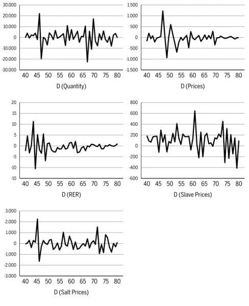
Heteroscedasticity analysis
Since the series presents evidence of heteroskedasticity, we use the loga-rithm transformation.
Figure A1 Heteroscedaticy analysis
20.000
10.000
0
-10.000
-20.000
-30.000
1.000
500
0
-500
-1.000
-1.500
D (Quantity) D (Prices)
40 45 50 55 60 65 70 75 80 40 45 50 55 60 65 70 75 80
30.000 1.500
10
5
0
-5
-10
-15
400
200
0
-200
-400
-600
D (RER) D (Slave Prices)
40 45 50 55 60 65 70 75 80 40 45 50 55 60 65 70 75 80
15 600
800 20
2.000
1.000
0
-1.000
-2.000
-3.000
D (Salt Prices)
40 45 50 55 60 65 70 75 80
A.2
Unit root tests
A.2.1 ADF - Dickey and Fuller
According to Dickey and Fuller (1981) for a sample size of 50 and probabi-lity of 0.95, the critical values for the constant and trend are, respectively, 3.14 and 2.81. Using information criteria (AIC, SIC and HQ) to select the number of lags, Table A1 presents the statistics for the model with tant and trend, while the third column is for the model with only a cons-tant. From these results, the model with constant and trend is not appro-priate for the variables LQ, LS and LSa, while the model with a constant is not appropriate for the variable LS.
Table A1 Statistics for trend and constant models Statistic (trend and constant)
Statistic (constant)
LQ @trend 1.009 LQ constant 4.309
LP @trend -2.923
LRER @trend -2.814
LS @trend -1.391 LS constant 2.073
LSa @trend -1.752 LSa constant 3.345
Using these different specifications, the following table presents the ADF unit root statistics for the five variables. Since the null hypothesis is for the existence of a unit root, we find evidence for a unit root in LRER and LS. The variable LP rejects the null at five percent but not at one percent. The variables LQ and LSA do not present evidence of unit roots.
Table A2 ADF unit root test
LQ LP LRER LS LSA
DF test statistic -4.221 -3.568 -3.012 -0.040 -3.351
Critical value (5%) -2.926 -3.508 -3.508 -1.612 -2.925
A.2.2 DF-GLS – Elliott, Rothenberg and Stock
Since the inclusion of deterministic terms may result in lower power for the ADF statistical test, we use the DF-GLS unit root test. We use this test with the variables LQ, LP, LRER and LSA, which have deterministic trends. The number of lags were selected based on the SIC criteria. Based on the test results, we find evidence for unit roots on the variables LQ, LP and LRER. The variable LSA is stationary.
Table A3 DF-GLS unit root test
LQ LP LRER LSA
ERS DF-GLS test statistic -0.855 -3.509 -2.752 -3.122*
Critical value (1%) -2.615 -3.770 -3.770 -2.615
Lag length (SIC) 1 0 0 0
A.2.3 KPSS - Kwiatkowski, Phillips, Schmidt and Shin
As a way to verify the previous results, we also used the KPSS unit root test. The null hypothesis of this test is that the variable is stationary. To select the model specification, we used graphical analysis of the variables, presented in Table A11. For lag selection, we used the Newey-West in-formation criteria with BarlettKernell as the spectral estimation method. The statistic also provides evidence that all variables, except LSA, have a unit root.
Table A4 KPSS unit root test
LQ LP LRER LS LSA
KPSS test stat const 0,663* 0,720* 0,841* 0,564* 0,336
Critical value C (5%) 0,463 0,463 0,463 0,463 0,463
KPSS test stat trend 0,190* 0,103 0,095 0,201* 0,109
Critical value T (5%) 0,146 0,146 0,146 0,146 0,146
Figure A2 Variables trends (log)
A.3
Lag criteria for the vector error correction model
With four variables I (1), the following table shows that one lag is an ade-quate selection for the model.
Table A5 VAR lag order selection criteria
Lag LogL FPE AIC SC HQ
1 30.50617 5.71e-06* -0.725308 -0.049757* -0.481050*
2 46.23700 5.89e-06 -0.711850 0.639254 -0.223334
3 60.43677 6.81e-06 -0.621838 1.404817 0.110936
4 74.20539 8.52e-06 -0.510270 2.191938 0.466763
5 88.04650 1.17e-05 -0.402325 2.975434 0.818966
6 104.8820 1.59e-05 -0.444102 3.609208 1.021447
7 113.4825 4.16e-05 -0.074123 4.654739 1.635684
8 169.1074 1.64e-05 -2.055368* 3.349046 -0.101303
Sample 1837-1884, 40 observations. Endogenous variables: LQ, LP, LRER, LS.
A.3.1 Johansen procedure
Based on the previous graphical analysis of the nonstationary variables, we assumed a model with a constant inside the cointegration vector and another on the VAR. Both the trace and maximum eingenvalue statistics indicate the existence of a cointegration vector.
10
8
6
4
2
0 12
183
7
1839 1841 1843 1845 184
7
1849 1851 1853 1855 185
7
185
9
1861 1863 1865 186
7
186
9
18
71
18
73
18
75
18
77
18
79
1881 1883
Table A6 Johansen cointegration vector test
Unrestricted cointegration rank test (Trace)
Hypothesized no. of CE(s)
Eigenvalue Trace statistic
Critical value 0,05
Prob. **
None * 0,557964 57,88214 47,85613 0,0043
At most 1 0,228640 20,32945 29,79707 0,4007
At most 2 0,118850 8,387854 15,49471 0,4249
Unrestricted cointegration rank test (Maximum Eigenvalue)
Hypothesized no. of CE(s)
Eigenvalue Max-eigen statistic
Critical value 0,05
Prob. **
None * 0,557964 37,55269 27,58434 0,0019
At most 1 0,228640 11,94159 21,13162 0,5534
At most 2 0,118850 5,820244 14,26460 0,6364
Sample 1839-1884, 46 observations. Series: LP, LQ, LRER, LS. Trend assumption: Linear deterministic trend.
Lags interval (in first differences): 1 to 1.
A.4
Residual test
For the residual vector to conform to the assumptions of the model, the residuals cannot be auto correlated and should have a normal distribu-tion. To test for autocorrelation, we used the LM test. For the normality hypothesis, we used the Cholesky test. The LRER and LS did not have normal residuals due to two outliers. Therefore, we used one dummy for the LRER variable for the year 1842 and another for the LS variable for the year 1883. The null hypothesis for the LM test is no serial correlation at lag order h.
Table A7 VEC residual serial correlation LM test
Lags LM-Stat Probability
1 17.87280 0.3314
2 19.64557 0.2366
3 10.52889 0.8376
4 15.75987 0.4698
5 11.97683 0.7456
Table A8 VEC residual normality test
Component Skewness Chi-sq df Probability
1 0.133134 0.135888 1 0.7124
2 -0.106905 0.087620 1 0.7672
3 0.266783 0.545660 1 0.4601
4 -0.272250 0.568254 1 0.4510
Joint 1.337423 4 0.8550
Component Kurtosis Chi-sq df Probability
1 1.731522 3.083984 1 0.0791
2 2.208278 1.201412 1 0.2730
3 1.917748 2.244931 1 0.1341
4 2.400673 0.688453 1 0.4067
Joint 7.218780 4 0.1248
Component Jarque-Bera df Probability
1 3.219873 2 0.1999
2 1.289032 2 0.5249
3 2.790591 2 0.2478
4 1.256707 2 0.5335
Joint 8.556203 8 0.3811
Sample 1837-1884. 46 observations. Orthogonalization: Cholesky (Lutkepohl). H0: residuals are multivariate normal.
A.5
Exogeneity tests
Since the cointegration coefficient of the variable LS is not different from zero, it can be stated that this variable is weakly exogenous. To reinforce this result, the LR test is carried out to the relationship between exoge-neity and cointegration.
Table A9 LR test
Cointegration restrictions: A(4,1)=0 (Convergence achieved after 9 iterations) LR test for binding restrictions (rank = 1)
Chi-square(1) 0.193767
The test statistic does not allow the hypothesis that the LS variable is weakly exogenous to be rejected. This implies, besides the existence of weak exoge-neity, that the variable has temporal precedence (Granger causality). As the results of the following table show, LS is not strongly exogenous.
Table A10 Granger causality test
NullHypothesis Obs F-Statistic Probability
D(LS) does not Granger Cause D(LQ) 46 0.04937 0.82521
D(LQ) does not Granger Cause D(LS)
APPENDIX B: Data
Table A11 VECM data
Year
Real Exchange Rate
Beef Jerky Quantity
Beef Jerky Prices (réis)
Slave Prices (mil-réis)
Salt Prices (réis)
1837 27.30 2,601 854.21 400.00 1.744
1838 25.02 2,360 681.09 500.16 1.689
1839 29.68 6,497 871.23 488.15 1.749
1840 26.49 5,959 821.95 453.94 2.047
1841 26.88 8,187 904.07 525.67 1.673
1842 38.14 9,932 697.61 612.49 1.951
1843 27.60 13,910 676.11 699.95 2.084
1844 32.80 11,888 676.04 448.74 4.354
1845 31.12 33,963 724.30 667.19 2.712
1846 27.76 14,496 1.942.26 630.15 2.404
1847 33.24 14,671 2.008.08 750.50 2.684
1848 26.45 13,138 1.082.96 505.20 2.690
1849 27.58 6,318 1.094.38 484.47 2.604
1850 28.95 10,515 1.688.48 426.44 2.929
1851 27.01 12,386 1.846.00 576.36 3.298
1852 24.34 10,541 1.596.34 547.02 2.757
1853 21.50 17,128 917.63 904.12 2.408
1854 20.82 16,387 705.07 946.60 2.457
1855 19.31 16,617 712.31 863.84 1.878
1856 18.05 18,436 575.77 996.75 1.600
1857 18.52 21,930 574.28 1.073.51 2.631
1858 17.12 14,559 668.22 1.152.45 2.528
1859 16.05 25,433 191.91 1.241.16 2.305
1860 17.38 22,808 469.77 1.038.67 2.991
1861 19.02 29,956 443.47 1.075.97 3.149
1862 17.92 28,341 346.82 1.699.21 2.609
1863 19.99 30,171 355.55 1.618.79 2.754
1864 16.93 35,952 442.69 1.254.50 2.223
1865 14.15 31,518 271.44 1.432.43 1.790
Year
Real Exchange Rate
Beef Jerky Quantity
Beef Jerky Prices (réis)
Slave Prices (mil-réis)
Salt Prices (réis)
1867 13.04 33,315 334.69 1.178.35 1.616
1868 10.82 43,748 250.11 1.326.12 1.383
1869 10.80 21,406 340.52 1.251.33 1.817
1870 10.40 27,190 290.46 1.202.58 1.412
1871 11.15 16,394 582.47 1.076.33 1.481
1872 11.80 33,513 247.28 1.125.64 1.741
1873 11.82 30,087 241.77 1.154.15 1.669
1874 11.50 22,491 236.74 1.287.86 3.188
1875 12.21 25,937 297.95 1.357.02 2.257
1876 10.95 23,847 303.69 1.762.62 2.172
1877 9.66 29,734 261.25 1.291.98 1.327
1878 9.92 28,005 242.05 1.545.01 2.145
1879 9.76 23,709 266.80 1.163.61 2.710
1880 10.36 24,575 321.97 1.281.42 2.388
1881 10.36 16,818 313.97 996.09 1.606
1882 10.32 19,130 238.82 1.049.31 1.622
1883 10.46 22,925 232.92 461.28 1.330
1884 11.59 22,644 221.62 459.51 1.454