❊♥s❛✐♦s ❊❝♦♥ô♠✐❝♦s
❊s❝♦❧❛ ❞❡
Pós✲●r❛❞✉❛çã♦
❡♠ ❊❝♦♥♦♠✐❛
❞❛ ❋✉♥❞❛çã♦
●❡t✉❧✐♦ ❱❛r❣❛s
◆◦ ✹✼✷ ■❙❙◆ ✵✶✵✹✲✽✾✶✵
❚❤❡ ❈♦sts ♦❢ ❊❞✉❝❛t✐♦♥✱ ▲♦♥❣❡✈✐t② ❛♥❞ t❤❡
P♦✈❡rt② ♦❢ ◆❛t✐♦♥s
P❡❞r♦ ❈❛✈❛❧❝❛♥t✐ ●♦♠❡s ❋❡rr❡✐r❛✱ ❙❛♠✉❡❧ ❞❡ ❆❜r❡✉ P❡ss♦❛
❖s ❛rt✐❣♦s ♣✉❜❧✐❝❛❞♦s sã♦ ❞❡ ✐♥t❡✐r❛ r❡s♣♦♥s❛❜✐❧✐❞❛❞❡ ❞❡ s❡✉s ❛✉t♦r❡s✳ ❆s
♦♣✐♥✐õ❡s ♥❡❧❡s ❡♠✐t✐❞❛s ♥ã♦ ❡①♣r✐♠❡♠✱ ♥❡❝❡ss❛r✐❛♠❡♥t❡✱ ♦ ♣♦♥t♦ ❞❡ ✈✐st❛ ❞❛
❋✉♥❞❛çã♦ ●❡t✉❧✐♦ ❱❛r❣❛s✳
❊❙❈❖▲❆ ❉❊ PÓ❙✲●❘❆❉❯❆➬➹❖ ❊▼ ❊❈❖◆❖▼■❆ ❉✐r❡t♦r ●❡r❛❧✿ ❘❡♥❛t♦ ❋r❛❣❡❧❧✐ ❈❛r❞♦s♦
❉✐r❡t♦r ❞❡ ❊♥s✐♥♦✿ ▲✉✐s ❍❡♥r✐q✉❡ ❇❡rt♦❧✐♥♦ ❇r❛✐❞♦ ❉✐r❡t♦r ❞❡ P❡sq✉✐s❛✿ ❏♦ã♦ ❱✐❝t♦r ■ss❧❡r
❉✐r❡t♦r ❞❡ P✉❜❧✐❝❛çõ❡s ❈✐❡♥tí✜❝❛s✿ ❘✐❝❛r❞♦ ❞❡ ❖❧✐✈❡✐r❛ ❈❛✈❛❧❝❛♥t✐
❈❛✈❛❧❝❛♥t✐ ●♦♠❡s ❋❡rr❡✐r❛✱ P❡❞r♦
❚❤❡ ❈♦sts ♦❢ ❊❞✉❝❛t✐♦♥✱ ▲♦♥❣❡✈✐t② ❛♥❞ t❤❡ P♦✈❡rt② ♦❢ ◆❛t✐♦♥s✴ P❡❞r♦ ❈❛✈❛❧❝❛♥t✐ ●♦♠❡s ❋❡rr❡✐r❛✱ ❙❛♠✉❡❧ ❞❡ ❆❜r❡✉ P❡ss♦❛ ✕ ❘✐♦ ❞❡ ❏❛♥❡✐r♦ ✿ ❋●❱✱❊P●❊✱ ✷✵✶✵
✭❊♥s❛✐♦s ❊❝♦♥ô♠✐❝♦s❀ ✹✼✷✮ ■♥❝❧✉✐ ❜✐❜❧✐♦❣r❛❢✐❛✳
The Costs of Education, Longevity and the Poverty of
Nations.
∗
Pedro Cavalcanti Ferreira
†Samuel de Abreu Pessôa
A bst r act
This paper explores the distortions on the cost of education, associated with govern-ment policies and institutional factors, as an additional determinant of cross-country income differences. Agents areÞnitely lived and the model takes into account life-cycle features of human capital accumulation. There are two sectors, one producing goods and the other providing educational services. The model is calibrated and simulated for 89 economies. WeÞnd that human capital taxation has a relevant impact on incomes, which is ampliÞed by its indirect effect on returns to physical capital. Life expectancy plays an important role in determining long-run output: the expansion of the popula-tion working life increases the present value of theßow of wages, which induces further human capital investment and raises incomes. Although in our simulations the largest gains are observed when productivity is equated across countries, changes in longevity and in the incentives to educational investment are too relevant to ignore.
K ey Words: Distortions, Human Capital, Longevity, Income Diversity
JEL Classification: J24, O11, O17, O47, O57
∗We gratefully acknowledge the comments and suggestions of João Issler, Marcos B. Lisboa, and several
seminar participants around the world. All remaining errors are ours. The authors also acknowledge the
Þnancial support of CNPq-Brazil and PRONEX
†Both authors are from the Graduate School of Economics ( EPGE ), Fundação Getulio Vargas, Praia de
1
I nt r oduct ion
This article studies the effects of distortions to factors accumulation, productivity and de-mography on cross-country income disparity. More speciÞcally, we explore the distortions on the cost of education, associated with government policies and institutional factors, as an additional determinant of income differences. As the model takes into account life-cycle features of human capital accumulation, the the long run impact of life expectancy on per capita income is also investigated.
We posit a continuous time overlapping generation model of capital accumulation with exogenous technological change and two sectors, educational and goods. All economies in the world have access to both technologies but they differ in their total factor productivity (TFP). Moreover, human capital is such that the skill level of a worker with TS years of
schooling is eφ(TS) greater (where φ is an increasing and concave function) than that of a
worker of the same cohort with no education at all. Life is Þnite in the model but average life span differs from country to country.
In this model there are two decisions made by individuals. First, at each instant of time they decide how much to consume or save out of their labor and capital incomes and public transfers. Second, they decide the optimal time to leave school. Following the labor-economics literature (e.g., Mincer (1974) and Willis (1986)), human capital investment is the time spent acquiring formal education plus the tuition cost. As usual, the longer people stay in school, the higher their stock of human capital is. At each moment, individuals weight the opportunity costs of being in school - the wages forsaken plus tuitions - against its beneÞt, which is the increase in the present value of wages due to higher human capital. One of the key variables to be considered in this decision is life expectancy, because the present value of the ßow of wages, everything else being the same, increases with longevity.
the end result of these distortions.
The model is calibrated in two steps. In the Þrst, we follow standard procedures and adjust the model to the US, estimating in the process productivity and the distortions to physical and human capital accumulation, among other variables. In the second step, a cross-section data set on schooling, investment ratio, life expectancy and labor force participation is employed, together with the technology and welfare parameters estimated previously for the US, to obtain the TFP, distortions and tuition costs for the remaining economies.
A Þrst Þnding of the paper is the relative importance of distortions to human capital accumulation. For comparable values, its effect on long-run income is of the same order of magnitude as that of distortions to physical capital accumulation. This is somewhat surprising in a model where education has no impact on the long-run growth rate and, as opposed to Lucas (1988) and Uzawa (1965), is a bounded variable which cannot be accumulated indeÞnitely. Education in the model determines skill levels and so it directly effects labor services and output. It also has an indirect effect on the latter due to its impact on the return to physical capital, and so on investment, a channel that multiplies the total impact of the taxes on education investment. In contrast, the educational sector uses very little capital - its capital share according to the NIPA is only 6 percent - so that the distortion to physical capital has almost no impact on human capital investment.
An unexpected outcome, and one that has received little attention, is the importance of life expectancy in the determination of long-run output. Greater longevity allows for extension of the population working life and, consequently, an increase in the present value of the ßow of wages of a given investment in education. Higher returns to education in turn induce individuals to stay in school longer, increasing average human capital and so long-run income. There is also an indirect effect on income prompted by physical capital accumulation, as the boost in human capital positively affects the return of the latter. We show that, everything else being equal, a country with life expectancy of 65 years instead of the 77 years of the benchmark case will have 23% less schooling, 26% less physical capital and its income will be 28% smaller in the long run.
countries such as France, were life expectancy is very high but schooling well below that of the US, those distortions were estimated as being higher.
The link between longevity and long-run incomes found in the model implies a channel from health policy to growth that has not been explored by the literature. Basic and cheap measures such as sanitation and preventive care are well known to have a huge impact on the welfare of populations. However, by increasing average life expectancy they indirectly effect the return to educational investment, which will induce further accumulation of human capital, boosting long-run income. Hence, theÞght against common Third World epidemics such as malaria, and more recently AIDS, not only has a direct beneÞt in terms of lives saved but also an impact on the long-run prospects of these economies that may well surpass the static loss of product due to deaths and diseases. In other words, in countries where life expectancy is too low, health and sanitation measures are probably the most effective growth policy.
To the best of our knowledge there has not been much interest in investigating long-run
level effects of distortion to human capital accumulation, especially using the Mincerian formulation of human capital. The macro literature has dedicated more effort to studying thegrowthimpact of human capital taxation, as in Trostel (1993), Stokey and Rebelo (1995), and Hendricks (1999). These papers employ the two-sector endogenous growth framework of Uzawa (1965) and Lucas (1988). However, in the face of recent empirical evidence (Bils and Klenow (2000) and Krueger and Lindhal (2000)) it seems that the growth effects of incentives to human capital accumulation is either very low or nonexistent. Additionally, as documented by Krueger and Lindhal, there is not a compelling set of evidence favoring the existence of externality associated to human capital accumulation. Our environment seems to be a conservative one for assessing the long-run importance of education and most likely we are underestimating the importance of schooling.
Mankiw (1995) and Parent and Prescott (1995) investigate the impact of distortions on long-run income for a version of the neoclassical model with three factors of production: raw labor, physical capital, and human capital (or organizational capital). In contrast to our model, they consider human capital and physical capital symmetrically, as stocks of goods that can be accumulated without limit. Another formulation of the neoclassical model of capital accumulation and exogenous technological change is Parent and Prescott (2000, chapter 4). Their set up however does not incorporate the life cycle features of educational choice, making the correspondence between the aggregate model and the micro data less precise.
This paper is organized in four sections in addition to this introduction. In the next section, the model is presented and in Section 3 we discuss the calibration procedures. Section 4 presents the main results and Section 5 concludes.
2
T he M odel
2.1
Fir m s
There are two sectors in this economy, one that produces consumption and investment goods and another that produces educational services. Let output Y1 in the Goods Sector be a
function of physical capital services K1 and skilled labor H1 according to:
Y1 =A1K1α(egtH1)1−α,
whereA1 is the sector total factor productivity andegtis the exogenous technological progress.
Skilled labor is given by:
H1 =L1eφ(TS)
whereL1is raw labor. According to the equation above, the productivity of a worker withTS
years of schooling iseφ(TS)greater than that of a worker of the same cohort with no education
at all. The function φ(TS) is assumed to be increasing and to exhibit diminishing returns,
and φ0(T
S)eφ(TS) gives the increase in effective labor input from one extra year of schooling.
This formulation follows the labor literature (e.g., Mincer (1974) and Willis (1986)), but has been used recently in the growth Þeld by Jones (2002) and Bils and Klenow(2000)
ProÞt maximization of the Þrm gives
where r1 is the rental price of capital and w1 is the wage rate, both in the Þrst sector, and
k1 ≡
K1
egtL
1eφ(TS)
, (1)
is the stock of capital in efficiency units.
The proposed technology of the Educational Sector takes into account that the produc-tion of educaproduc-tional services is labor intensive. For instance, capital’s share in income of educational services sector was only 6.2% in1997, according to the Survey of Current Busi-ness, published by the U.S. Department of Commerce. In this sense it will be assumed that schools employ only labor and that there is no technological progress in the sector.1 The
production function of the sector is:
Y2 =A2H2 =A2L2eφ(TS)
and wages are
w2 =eφ(TS)A2.
2.2
H ousehold
Suppose a household that is born at time s and faces a life span of T years. Life has three different periods: youth, TY, adulthood, TW, when working, and old age, TR, after
retirement. Youth has two sub-periods: childhood,TC, when staying at home, andTS, when
at school.
At each instant of time the household decides how much to consume or save out of labor and capital incomes and public transfers. A decision is also made on how much education to buy, which is equivalent in the model to deciding the optimal period of time TS of staying
in school. The utility function of an individual born at time s is:
Z s+T
s
e−ρ(t−s)c(s, t)1− 1 σ −1
1−σ1
dt, (2)
wherec(s, t)is the consumption attof an individual born ins, whileρandσare respectively the discount rate and the intertemporal elasticity of consumption.
1This last assumption is necessary for a balanced growth path in which tuition increases at a rate equal
Individuals have 3 sources of income - wages from labor services, rents from capital and public transfer - which is used to pay for school tuition and consumption goods. In intertemporal format their budget constraint is given by:
Z s+TY+TW
s+TY
e−r(t−s)w(s, T
S, t)dt+
Z s+T
s
e−r(t−s)χ(s, t)dt (3)
=
Z s+T
s
e−r(t−s)c(s, t)dt+ (1 +τ H)
Z s+TY
s+TC
e−r(t−s)ηq(t)dt,
where r is the interest rate, w(s, TS, t) is the wage in time t of a worker born at s with
TS years of formal education and χ(s, t) is the government transfer at t toward a cohort-s
individual. The last expression on the right hand side is the tuition costs, where τH is a tax
(or subsidy) rate on education purchases,ηthe amount of education services that the student has to buy in order to be in school,2 andq(t) is the price of one unit of educational services
in units of consumption goods. The above expression simply says that the present value of wages and government transfers should be equal to the present value of consumption and tuition costs. Note also that tuitions are not proportional to wages, a point we will elaborate later.
Individuals maximize(2)subject to (3).Solving for consumption, we obtain the individ-ual’s consumption proÞle:
c(s, t) =c(s, s)eσ(r−ρ)(t−s). (4)
Let w(s, TS, t) = ω(t)eφ(TS), where ω(t) are the wages for raw labor. Moreover, as we
are interested in studying the model’s solution at a balanced growth path in which income, transfers, and tuition grow at the same constant rate g, we will assume that ω(t) = ωegt,
q(t) =qegt and χ(s, t) =χegt. With these simpli
Þcations we obtain an expression for initial consumption, after substituting (4) into (3):
c(s, s)
υa
= e
gs
r−g ©
ωeφ(TS)e−(r−g)TY ¡1
−e−(r−g)TW¢ (5)
−(1 +τH)e−(r−g)TC
¡
1−e−(r−g)TS¢η
q+χ¡1−e−(r−g)T¢ª .
2We are assuming an indivisibility in the human capital accumulation process. In order to increase
The right-hand term is the individual’s total wealth at the time of birth (i.e., labor income less tuition plus government transfers) and
υa=
(1−σ)r+σρ
1−e−((1−σ)r+σρ)T
is the propensity to consume out of initial wealth.
In this economy, the education decision is equivalent to choosing the optimal time to leave school. In the beginning of their lives, individuals pick the optimal quantity of education in order to maximize the present value of income:
max
TS
½Z s+TY+TW
s+TY
e−r(t−s)w(s, T
S, t)dt−(1 +τH)
Z s+TY
s+TC
e−r(t−s)ηq(t)dt
¾ .
In making this decision, individuals consider that the longer they stay in school, the shorter their productive life, TW, as retirement age TR is exogenous. Moreover, in addition
to the foregone wages, there is the direct cost of school tuition. Using again ω(t) = ωegt,
q(t) =qegt andχ(s, t) =χegt,and the fact thatT
Y +TW =T−TR,we can write the optimal
choice of education as:
max
TS
½
ωeφ(TS)e
−(r−g)TY
−e−(r−g)(T−TR)
r−g −(1 +τH)ηq
e−(r−g)TC
−e−(r−g)TY
r−g
¾ .
Remember that agents born at s stay in school froms+TC to s+TY (= s+TC +TS)
so the expression on the right gives the present value of total tuition costs, while the one to the left gives the present value of labor income.
From theÞrst order condition of this problem at a balanced growth path we obtain:
ωeφ(TS)φ0(T S)
1−e−(r−g)TW
r−g =ωe
φ(TS)+ (1 +τ
H)ηq. (6)
The expression above equates the present value of staying in school one additional unit of time (the left-hand side) to the opportunity cost of not working plus the tuition cost at the stopping time (the right-hand time). Note that dividing both sides of equation (6) by
(1 +τH) one can see that tax on tuition is equivalent to direct taxation on wage income.
Note also that if it was not for the tuition term, human capital taxation or taxes on wages would have no impact at all. In the latter case, a tax term (1 +τH) would divide both the
model, the taxation term would be eliminated. Hence, the education decision would not be affected by taxation or distortions.
It is assumed that at each instant a cohort of size 1
T is born. Consequently, the total
population is equal to 1. Let us call NC, NS, NW, and NR respectively the population of
children, students, workers, and retirees. It will be assumed that the student-population ratio is proportional to the ratio of years of education to life span:
NS
N =NS = TS
T . (7)
Likewise, we posit that:
NC =
TC
T , NW = TW
T andNR= TR
T . (8)
2.3
G over nm ent R est r ict ion
Government revenue is given by the sum of taxation of educational services and capital income, so that the government budget constraint is:
τHηq(t)NS +τKr1K(t) =χ(t).
2.4
A ggr egat e Consum pt ion
Before presenting the equilibrium conditions of this economy, we need to derive an expression for aggregate consumption, which is done by adding the individual consumption over cohorts:
C(t) = 1
T Z t
t−T
c(s, t)ds. (9)
Equation (4) provides the consumption proÞle for an individual. If initial consumption, due to technological change, increases at a rate g, so thatc(s, s) =xegs, we obtain
C(t) = x1 T
Z t
t−T
egseσ(r−ρ)(t−s)ds
= xe
gt
T
1−e−(g−σr+σρ)T
From (5) and (10) it follows that:
c ≡ C(t)
egt = υc
T (r−g)
©
ωeφ(TS)e−(r−g)TY ¡1
−e−(r−g)TW¢ (
11)
−(1 +τH)ηqe−(r−g)TC
¡
1−e−(r−g)TS¢+χ¡1
−e−(r−g)T¢ª .
where υc is a positive constant that depends on υa and other parameters.3 This expression
simply says that aggregate consumption in each period is a fraction of the permanent income of the representative agent.
2.5
L ong-R un G ener al Equilibr ium
The following equations describe the long-run equilibrium of this economy along the balanced growth path.
The equilibrium in the market for educational services is:
A2(1−l1)NWeφ(TS)=ηNS, (12)
where l1 is the fraction of the total labor force employed in sector one.
The equilibrium in the assets market implies that
r= (1−τK)r1−δ= (1−τK)αA1k1α−1−δ, (13)
whereτK is a tax rate on capital income. From the above expression we obtain the following
equation that will be useful later:
k1 =
µ
1
αA1
r+δ
1−τK
¶ 1 α−1
. (14)
Free labor mobility across sectors implies equality of wages in sectors one and two, both in units of good one:
w1 =egtω =egt+φ(TS)(1−α)A1k1α=qegt+φ(TS)A2 =q(t)w2.
Under a balanced growth path, this last equation simpliÞes to
ω ≡ ω(t)
egt = (1−α)A1k
α
1 =qA2. (15)
3More exactly,υ
c= υa∗ 1−e
−(g−σr+σρ)T
The government budget constraint, in which revenue is given by the sum of taxation of educational services and capital income:
τHηq(t)NS+τK
r+δ
1−τK
K(t) =egt
µ
τHηqNS+τK
r+δ
1−τK
k ¶
=egtχ, (
16) where (r+δ)/(1−τK) = r1 is the rental price of capital and follows from (13), and k ≡
K/egt.
The goods market equilibrium is:
c=A1l1NWeφ(TS)kα1 −(δ+g)k, (17)
where c is given optimally by equation (11), after the expression for government transfers above is plugged in.
Finally, after substitutingω =A2q, the equilibrium conditions with respect to the
edu-cational choice are:
A2 η e
φ(TS)
½
φ0(TS)
1−e−(r−g)TW
r−g −1 ¾
= 1 +τH. (18)
An important result that will be useful later can be seen from the equation above. The only channel between the distortion to capital accumulation (or the productivity of the goods sector) and the educational choice is through the interest rate, net of distortion, r. If the economy is open, such that r is given internationally, the educational choice will not be affected by changes inτK. The same is true if the economy is closed but the long-run solution
for r is not very sensitive to the distortion to capital accumulation (nor to the productivity of the goods sector). In both cases the education choice, in general equilibrium, depends mainly on τH. The same does not happen with the capital decision: changes in τH have a
considerable impact on k through their effect oneφ(TS).
3
Quant it at ive M et hodology
The calibration of the model is carried out in two steps. First, the model is calibrated to the US. In the second step we assume that the economies in our data set share with the US the same values for preferences and technological parameters. Then, using some observable variables for each economy, we get the implied (or measured) values for the incentive parameters, τK and τH, and for productivity, A1. We use the calibrated model to
3.1
Calibr at ion
The function φ(TS) is taken from Bils and Klenow (2000):
φ(TS) = θ
1−ψT
1−ψ
S . (19)
According to their calibration, we have ψ = 0.58and θ = 0.32. Hence, instead of the more usual linear return to education assumed in most of the literature, we posit diminishing returns because this seems to be the case when comparing micro estimates across countries.4
We will also consider the following parameters as observable:
l2, TC, TS, TW, T, g,α, r,δ,σ.
The share of labor in the educational sector, l2, was obtained from the NIPA and is
the average from 1987-1997 of the ratio of Full-Time Equivalent Employees in Educational Services to the Total Full-Time Equivalent Employees and was found to be 1.6%. For T we used the life expectancy in 1995, obtained for all countries in World Bank (1990). However, as the relevant educational decision is taken not at birth but some years later, we constructed an adjusted life expectancy series, conditional on survival to the age of Þve.5 T
W was found
using equation (8). In this case NW was constructed using labor force and population data
from World Bank (1990).
The capital share in the goods sector was set equal to one-third, which is the number found in the NIPA. The interest rate was set at 4.5%, depreciation at 6.6%,6 the exogenous
growth rate g equal to 1.36% a year7 and the investment-output ratio to 0.18, the average
value for the variable in the Summers and Heston database from 1975-1995. TS for all
economies corresponds to data on years of schooling attained by the working-age population from the Barro and Lee (2000) database.
There are six parameters left to be found:
A1,
A2
η ,ηq,τK,τH andρ,
4In addition, the value 0.58for ψprovides ‘enough’ concavity ofφ(T
S). See the discussion in Appendix
B.
5We used the World Bank series Infant Mortality Rates (for children under one year old), Under-5
Mortality Rates and Life Expectancy at Birth to construct the adjusted life expectancy series.
6This is a long-run average for the investment/capital ratio, as given by NIPA, both evaluated at market
prices.
which will be estimated solving equations (12), (15), (17) and (18), the model’s value for output
y=NWeφ(TS)(A1l1kα1 +qη
A2
η l2), (20)
and the investment-output ratio
i y =
(δ+g)k
NWeφ(TS)(A1l1k1α+qηAη2l2)
, (21)
considering y and i/y as observable. Both were obtained using updated Penn World Table Mark 6.0 data for the year of 1995. Finally, we assume logarithmic preferences, so thatσ is set equal to 1.
3.2
Cr oss-Count r y I ncent ive and P r oduct ivit y M easur em ent
In order to get the implied values of τK, τH, A1 for the remaining economies in our data
set, we assumed that the economies share with the US the same preference, technology and return to education parameters. Hence, the values for the following exogenous parameters:
{θ,ψ,ρ,σ,α,δ},
are those calibrated for the US. Moreover, g, r andA2 are also equal across economies.8
Finally, with the help of cross-section data from the same sources for T, y, and i y, we
solve (12), (14), (17), (18), (20), and (21), for{A1,ηq,τK,τH, l2, k}.
We are left with the calibration of the time spent in the job market, TW, which, given
the assumption of exogenous retirement life, is equivalent to the calibration of TR. We use
population and labor force data from the World Development Report (World Bank1990) to calibrate TR such that the model’s value for
NW
N = TW
T
reproduces the data.9 In other words, in this model the ratio of working time to life span is
equal to the ratio of labor force to total population. We use data on NW/N andT to obtain
TW andTR.
8Given that the educational sector almost only employs labor,eφ(TS) already controls for TFP differences
in this sector.
In this subsection, in order to identifyτK we assumed that the the interest rate, free of
distortion and risk, is the same across economies. Consequently, we are assuming capital mobility. Given that we do not have data for the difference between internal output and domestic income, we are implicitly assuming, when employing (17), that the net external debt is zero.
3.3
Simulat ion of t he M odel
We will later perform an experiment to evaluate the sensitivity of the endogenous variables to modiÞcations in the parameter values. In particular we are interested in evaluating the relative impact on long-run per capita income of changes in
{A1,τH,τK, T}, (22)
keeping Þxed all other parameters (in particular, when we changeT we hold TR
T constant).
In this exercise we assume that the economy is open, so that we considerr= log(1.045)
as given for every combination of (22). We then solve (18) to get TS, and, consecutively:
(12) for l1, (14) for k, (15) for q, and (20) for per capita income. Finally, the difference
between internal output and domestic income is given by the solution of (17), which is not necessarily zero now.10
4
R esult s
4.1
M easur em ent of pr oduct ivit y and dist or t ions t o fact or
accu-mulat ion
We are interested in understanding how differences in distortions to factors accumulation and productivity affect long-run income disparity across countries. In our model, everything else being the same, large τK and/orτH and small A1 imply smaller per capita income. As
in the long run all countries grow at the same rate g,these differences are permanent.
10The fact that in the open economy solution of the model equation (17) is a residual equation used to
In estimating ofτK,τH,andA1in the 89 countries in our sample, we found wide variations
of these variables. Taking the US as the benchmark economy, so that we set {qUS, A1US} = {1,1} and{τHUS,τKUS}={0,0}, τH in Mozambique and Niger, for instance, was found to
be 0.88 andτK in Rwanda and Haiti 0.85, while being -0.17 in Argentina and -0.74 in Japan,
respectively (hence, a relative subsidy in both countries). More interesting, the estimated correlations among τK, τH, A1 are relatively small: it is 0.22, between τK and τH; −0.40,
between τK and A1; and −0.33, between τH and A1. The low correlation between τK and τH,for instance, implies that an economy with good incentives to capital accumulation, and
hence with high investment ratio, may also have very low observed schooling levels due to high taxation of education.
We estimated Þve countries as being marginally more productive than the US: Italy, France, Singapore, Belgium and Mauritius. On the other hand, there are countries such as Tanzania (the least productive in our sample), China and Togo where Total Factor Produc-tivity (TFP) is one quarter or less of US producProduc-tivity. The TFP ratio of the most productive to the least productive country is 6.1. These results are similar to those in Hall and Jones (1999), among others.
Table 1 below presents the estimated levels of τK, τH and A1, relative to the US for a
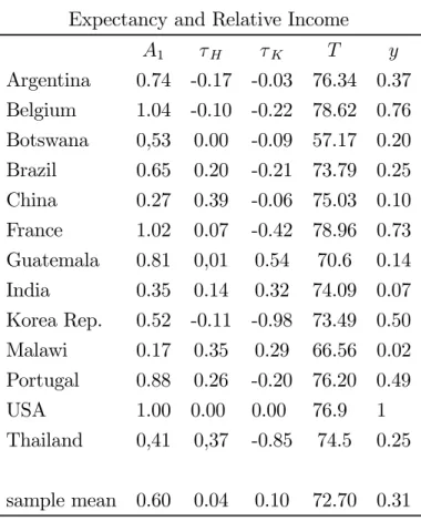
Table1: Productivity, Distortions, Life Expectancy and Relative Income
A1 τH τK T y
Argentina 0.74 -0.17 -0.03 76.34 0.37 Belgium 1.04 -0.10 -0.22 78.62 0.76 Botswana 0,53 0.00 -0.09 57.17 0.20 Brazil 0.65 0.20 -0.21 73.79 0.25 China 0.27 0.39 -0.06 75.03 0.10 France 1.02 0.07 -0.42 78.96 0.73 Guatemala 0.81 0,01 0.54 70.6 0.14 India 0.35 0.14 0.32 74.09 0.07 Korea Rep. 0.52 -0.11 -0.98 73.49 0.50 Malawi 0.17 0.35 0.29 66.56 0.02 Portugal 0.88 0.26 -0.20 76.20 0.49 USA 1.00 0.00 0.00 76.9 1
Thailand 0,41 0,37 -0.85 74.5 0.25
sample mean 0.60 0.04 0.10 72.70 0.31
Before performing a systematic analysis of the impact of incentives and productivity on cross-country income differences, some comments on the parameters estimation may be illustrative. India, China and Guatemala are relatively poor or very poor countries. However, the reasons vary. Guatemala, among other reasons, is relatively rich in natural resources and hence its estimated productivity is very large. Its incentives to physical capital accumulation, however, are extremely low, among the worst in the sample. The estimated productivity in India and China, on the other hand, is well below the sample mean and in both cases distortions to human capital investment are high and above the sample mean. However, τK
in China is very low. Malawi fares very badly in every possible aspect and there is no wonder it is one of the poorest countries in the world.
South Korea’s strength is capital accumulation and education, but it has below-average productivity for world standards. Similar stories could be told with respect to Malaysia and to a lesser extent Japan (where estimatedA1 is above average but only 80% of the US level).
very good at setting the right incentives to physical capital accumulation and its estimated
τK is the second smallest in the sample, after Singapore.11
For our purposes, the case of Portugal is of great interest. Portugal is a middle income country as its GDP per capita is only 49% of the USÞgure. Its estimated productivity is12% below the leaders but well above average. Its incentives for physical capital accumulation are estimated as being better than American incentives. However, the distortions to human capital investment are very high, being the 16th. worst in the sample: Portugal has the same life expectancy as the US but only 46 percent of its educational attainments. A similar case can be made for France, which is much richer than Portugal but also has above average
τH. In this case both productivity andτK are better than in the US, but due mostly toτH,
France is only 75 percent as rich as the US. Again, low schooling is the explanation12.
Schooling in Botswana, in contrast, is low, less than 6 years, but its estimated incentives for the accumulation of human capital are better than average, superior to many rich and more educated countries. Note, however, that life expectancy in Botswana is very low, 57 years, almost 20 years less than the sample median. The next section explores the link between longevity, education and development.
4.2
T he I m pact of L ife Expect ancy
One unexpected outcome of the simulation of the model is that in a group of poor or relatively poor countries with little education, the estimated values ofτHare not very high. Indeed, not
only for Botswana, but for countries such as Zambia, Lesotho and Zimbabwe, the estimated value of this variable was below average and even below those of many rich economies. However, schooling in all four cases is below average.
The apparent contradiction between little observed education and good estimated
incen-11In Belgium,τ
K andτH are both smaller than in the US and productivity is larger. Income, however, is
30% smaller. The reason for this apparent puzzle is labor-force participation, which is 49% of the working-age population in the USA, while only 40% in Belgium. Hence, part of the income per capita difference is due simply to a larger proportion of workers in the population in the US, which in the model simulation is an exogenous parameter that varies across countries. In our calibration, TW is proportional to labor-force
participation. This is also an important factor explaining the relative income of France, Argentina and Brazil, among other countries.
12Recall that in our framework τ
H is equivalent to high payroll taxation. Hence, in the case of France,
tives is explained mostly by longevity. In a country in which agents do not expect to live long, the optimal decision is to stay in school for very few years. Remember that in this model, while in school agents are out of the labor market. Hence, the shorter the number of years that an agent expects to beneÞt from investing in education, the sooner is the optimal time to leave school. In the case of Lesotho, for instance, schooling is only 4 years but life expectancy is also very short, 52 years, so that the estimatedτH is very small. With such a
short life, 4 years of education is not a bad record13. On the other hand, rich countries with
high life expectancy but relatively less education than the leaders have large estimated τH.
As we just saw, in France the estimated value of this variable was 0.07, above the sample average, while life expectancy in1995 was the same as in the US. Educational attainment of the French working age population in1995, however, was only 62% of that of the American working age population (but 23% above the average level in our sample), an indication that distortions to human capital investment in France are comparatively large. Hence, the best performers in this case are not necessarily the ones with the highest schooling levels, but those with relatively high schooling with respect to life expectancy.
Once we control for longevity, this result no longer holds. If we keep education level constant in Botswana, but give the US life expectancy to its population (holding TR/T
constant), its estimated τH jumps to 0.10. In Lesotho it goes from -0.028 to 0.15. Hence,
the correlation betweenτHand education, given observed life expectancy, is−0.50. However,
this correlation is considerably higher in absolute value, −0.65, when we set each economy to US life expectancy. This result indicates that policies that increase longevity may have a considerable effect on output, as they raise the incentives to the acquisition of education.
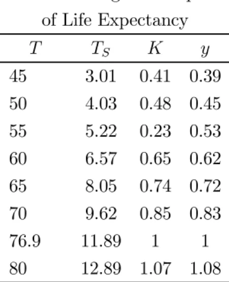
In order to better understand the relationship between long-run income and longevity, in Table 2 below we present the result of the simulations of the model holding all parameters constant at the values estimated and calibrated for the US, at the same time that we vary life expectancy numbers:14
13Had we not adjusted life expectancy and used life expectancy at birth for T, we would get τ
H= −0.06
for Angola, a country with only 2.4 years of average education. In this case, life expectancy is only 45 years, so that productive life is extremely short, as is the return of a given investment in education. The observed education level, although small in absolute terms, is too high with respect to the expected return, which explains the negative τH.
14In this exercise we adjusted the retirement time in order to keep TR
T constant. See subsection 3.3 for the
Table 2: Long-Run Impact of Life Expectancy
T TS K y
45 3.01 0.41 0.39 50 4.03 0.48 0.45 55 5.22 0.23 0.53 60 6.57 0.65 0.62 65 8.05 0.74 0.72 70 9.62 0.85 0.83 76.9 11.89 1 1
80 12.89 1.07 1.08
As life expectancy decreases, the number of years of education decreases monotonically. If instead of 76.9 years, life expectancy in the US was only 65 years (in line with South Africa and Lesotho, for instance), the equilibrium amount of education would decrease from
11.9 years to 8.05. With life expectancy as low as in Rwanda, schooling would drop to only 3.15 years in the US. This fall in education has a direct effect in output per worker, through the eφ(TS) component of the production functions of both sectors. However, it also has a
considerable impact on physical capital. In the case of T = 55, optimal k would be only 43% of the benchmark case. The explanation is straightforward: the decrease in education reduces the return to physical capital, consequently decreasing investment and its long-run stock.
The total effect on output per worker is considerable: the model predicts that a country equal to the US in everything but with seven fewer years of longevity in the long run would be 17% poorer. In fact, we estimated that the output elasticity to life expectancy is quite high, around1.7. The elasticity of schooling with respect to the same variable is even higher, 2.5. In other words, the model predicts that a country currently with T = 60 and TS = 5,
4.3
T he I m pact of D ist or t ions t o Educat ion and Physical Capit al
A ccumulat ion
In this section we study the sensitivity of the model to modiÞcations in the two distortion parameters. Additionally, we are also interested in comparing their relative impact on long-run income. On the one hand, capital is an unbounded variable, but subject to decreasing returns; on the other hand, due to a Þnite life-span, human capital is bounded, but this counteracts the concavity of the production function. Finally, to some extent, the distortion to human-capital accumulation is tax-neutral (wage taxation also reduces the opportunity cost of being in school rather than in the labor market). Consequently, it is not clear which distortion is more harmful to long-run income or if their order of magnitude is even comparable. In order to asses this we have to make τH and τK comparable. We deÞne
τEH ≡ τH
1 +τH
,
where τEH stands for ‘equivalent.’ It is theßow-equivalent taxation on labor.15
Table 3 below presents the results of an exercise in whichτEH varies and everything else is kept constant at the benchmark values:
Table 3: Long-Run Impact of Human Capital Taxation
τE
H TS K y
-0.3 14,97 1,14 1,24 -0,15 13,67 1,09 1,14 0 11.89 1 1
0,15 9,28 0,86 0,81
0,30 5.65 0,65 0,56 0,50 1.80 0,39 0,31
0,65 0,64 0,28 0,22
15If instead of considering taxation on tuition we had considered taxation on wages, τE
H would be the tax
rate that would reproduce the same economic incentive to human capital accumulation. In other words, in equation (6) instead of (1 + τH) multiplying the ηq term, we would have (1−τEH) multiplying the 2
As already said, distortions were normalized to zero in the US. In addition to the direct impact on education, τEH also affects physical capital accumulation through the negative im-pact on its return. Hence, an economy withτEH = 0.30will have less than half the education and 65 percent of the physical capital of the US, even with the same productivity, τK and
longevity. Its income per worker will be 44 percent smaller. There are 12 countries with estimated τE
H around or larger than 0.30 (13 percent of the sample). With distortions such
as that estimated for Niger and Mozambique (τE
H ≈0.50) there is practically no incentive to
education investments: agents would accumulate less than two years of education and conse-quently income per capita would be less than a third of the US income. On the other hand, negative τEH, “subsidy,” induces agents to accumulate more education than the US, but the
Þnal effect on income is proportionally smaller: an economy with τEH = −0.30, everything else the same, would be only 24% richer.
The qualitative impact of τK on long-run output is similar to τH, as it impatcs income
negativelly. There are, however, important differences. In our model, there is no physical capital in the production function of the educational sector. Hence, TS does not change with τK, since the Þrst order condition with respect to educational choice is not affected by it.
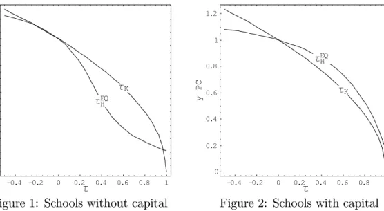
For comparable values, the impact of distortions to investment in education on income per capita and per worker is of the same order of magnitude but marginally larger than that of distortions to physical capital accumulation, as is clear from Figure 1.
This quantitative result is not robust to modiÞcations to the production function of the educational sector. We repeated the steps of Sections 2 and 3 for a version of the model with physical capital in both sectors, but without technology progress (otherwise the price of education would approach zero assymptotically). The capital share in the educational sector was set to 0.065, which is the average Þgure in the NIPA for the last ten years. All other parameters were those of Section 3 with minor adaptations.16 The overall simulated
effect of τK over the long-run income is now marginally larger than that ofτH, as shown by
Figure 2 below.
16Actually, calculations are more complicated in this case. This is the main reason we opted to work
-0.4 -0.2 0 0.2 0.4 0.6 0.8 1 J
0 0.2 0.4 0.6 0.8 1 1.2
y
C
P JK
JHEQ
Figure1: Schools without capital
-0.4 -0.2 0 0.2 0.4 0.6 0.8 1
J 0
0.2 0.4 0.6 0.8 1 1.2
y
C
P JK
JHEQ
Figure 2: Schools with capital
Distortions to the accumulation of physical capital now have a direct effect on both sectors and an indirect effect on the returns to educational investment and, for this particular parametrization, its impact on income is larger than that of τH. However, magnitudes are
similar and the impact of distortions to human capital investment on long-run income is still sizable. The relevant result is that in an economy in which there are other costs to education than foregone wages, distortions to investment in human capital have a large impact on long-run output and relative incomes, comparable to that of distortions to physical capital accumulation. Moreover, as shown in the case of Portugal in Table1, the measuredτH0sare
such that they may explain a large fraction of the distance of poor economies to the leading countries.17
Results concerning productivity differences are as expected. An economy equal in every aspect to the US but with only 50% of its productivity would have only 30% of the income per capita of the latter. If the country TFP was just 20% of that of the US, the smallest estimation in our sample, this economy’s income per capita would be 9% of the American income. Hence, in this model productivity can explain a large part of the income disparity across countries. In fact, the elasticity of output per capita with respect to A1 is 1.5. This
result is exactly what the standard neoclassical model of capital accumulation - inÞnite horizon and exogenous technological change - delivers18 and the same as those in Jones
17An estimated τ
H of 0.43 corresponds to τEH = 0.30. From Table 2 we can conclude that educational
distortions alone in Portugal explain almost half the gap with the US income.
(1997) and Hall and Jones (1999).
4.4
Count er -fact ual exer cises
In a group of simulations we substituted in all economies, one at a time, τK, τEH, A1 and
T (life expectancy) with the 9th-best estimated value of each parameter, which divides the
Þrst from the second best decile. We did this to avoid outliers that would occur if we had used the best estimated parameter.19 In each exercise we held labor force participation (and
the ratio TR/T)constant. Table 4 below presents the results.
Table 4: Counter-factual exercises on relative income per worker
original substitute by the 9th best value:
τk τh A1 T
Mean 0,328 0,388 0,420 0,504 0,351
Variance 0,085 0,089 0,145 0,081 0,087 Coef. of Variation 0,259 0,228 0,345 0,160 0,247
We observed the largest gains in per worker income when substituting the 9th-best pro-ductivity in all economies. In this case, mean output per worker goes from 33 percent to 50.4 percent of the US per worker income. Although smaller, the average change obtained from the simulations with τH is signiÞcant: mean output per worker increases by 28
per-cent if instead of their own inper-centives for human capital accumulation, all countries had the 9th-best τH.The same exercise with τK delivered an average gain of 18 percent in long-run
output per worker. The highest fall in dispersion (as measured by the variance-mean ratio) is obtained when A1 is normalized.
Although it is true that policies aimed at increasing productivity apparently have the potential to deliver the highest average payoffs, better incentives to the acquisition of ed-ucation also have a high return. This is even more apparent when we look at individual countries.
economy (cross-country equalization of the interest rate net of risk and distortion), and also because the share of the educational service in total output is very low.
19We did not use American parameter values because its estimated τ
H is close to the mean, while
It has been shown previously that schooling in France is considerably less than in the US, but that life expectancy is equal and output per worker not too different (73% of the US level, according to the Summers and Heston database). Hence, the estimated τH was
relatively high (0.07), while its performance in terms of A1, and τK was good. If France
were given the same incentives to human capital accumulation as that of the US, the model predicts that its output per worker would jump to 90% of the American GDP per worker, given the new schooling and capital levels implied by the new τH. Notice that in a model
with exogenous human capital accumulation, this fact would not be noted, as education level in France is relatively high by world standards.
The impact on Portugal is even more dramatic: its GDP per capita would jump from 44 percent of the US GDP to 69 percent if it were given American incentives to invest in education. In this case, schooling would jump from 5.47 years to 8.68 years. Of course, most poor countries would also beneÞt from better educational incentives, and in some cases like Mozambique and Bangladesh GDP per capita would be twice as large as observed.
Given the life-cycle structure of our model, drastic modiÞcations in longevity have a potentially large impact on long-run income. Average adjusted life expectancy in Sub-Sahara Africa is 64.7 years in our sample. The model predicts that GDP per worker would be 42 percent higher, on average, if African countries had American longevity (77 years). In the case of Zimbabwe, relative output per worker would increase from 10.8 percent to 18.7 percent of the US output, while schooling would go from 5.4 to10.9 years, which is expected given the low estimated τH of this country. Similar results are observed in countries such as
Botswana, Rwanda, Kenya and many others. In this group, the output gains are higher or close to those that would be obtained if their estimated TFP was substituted with American TFP. Although on average the largest gains are observed when TFP is substituted in (African countries in general are not too productive), changes in longevity and also in the incentives to educational investment are too relevant to ignore.
5
Conclusion
into the growth literature as well, e.g., Bils and Klenow (2000). In this formulation, the skill level of workers is an increasing function of schooling and the accumulation of skills is mostly done at school, outside the labor market.
This framework contrasts with the usual Uzawa-Lucas formulation where there is no bound on the accumulation of human capital, which is continuously acquired during the worker’s inÞnite life. Moreover, in general in the usual Uzawa-Lucas models there are no other costs of investing in human capital, such as tuition, than the forgone wages.
Investigation of the general equilibrium effects of distortions to human capital accumu-lation showed that they have a multiplicative impact through their effect on savings and physical capital. As investment in education falls because of taxation (or due to any other distortion), and with it the long-run stock of human capital, the return to physical capital also decreases, inducing individuals to reduce their investment. Our simulations showed that for reasonable parameters values, human capital taxation may be more detrimental to long-run income than taxation of physical capital. The literature on the latter, however, is much more extensive than that on the former, although there are important exceptions, most of them using endogenous growth models. One possible reason is that taxation on human capital in many models is neutral, as it decreases the return to human capital but also the cost of being out of the labor market. However, our results show that if there are any other costs imposed on the acquisition of education which are not proportional to wages (e.g., tuition), the long-run impact of taxation on human capital is relevant.
A
A pp endix: A N ot e on t he R et ur n t o Educat ion
In this paper, education modeling derives from the human capital literature of Schultz, Becker and Mincer. A very important concept in this tradition is the Social Marginal Internal Rate of Return (SMIRR) of TS years of education, which is deÞned as the discount rate R such
that the present value (PV) of wages minus the PV of tuition is equal to the PV of wages minus the PV of tuition when the individual stays TS+∆t years in school (Willis, 1986. p.
531). Formally,
ωe−(r−g)TSeφ(TS)1−e
−(R−g)TW
R−g −ηq
1−e−(R−g)TS
R−g
= ωe−(r−g)(TS+∆t)eφ(TS+∆t)1−e
−(R−g)(TW−∆t)
R−g −ηq
1−e−(R−g)(TS+∆t)
R−g .
After taking a Taylor expansion up to the Þrst-order term and taking the limit for ∆t → 0
in this last expression we get (6) for R = r if τH is zero. In other words, if there is no
distortion to the acquisition of education, at the market equilibrium the SMIRR is equal to the market interest rate.20
With the help of the concept of SMIRR, we can calculate the difference between the private rate of return and the social rate of return. The SMIRR of TS years of schooling for
a given economy is the value of R that solves
ωeφ(TS)φ0(T S)
1−e−(R−g)TW
R−g =ωe
φ(TS)+ηq.
The private rate is the market interest rate. Consequently, the distortion to the human capital accumulation decision is
τIH =
R−r R ,
or, rearranging terms, it is the implicit tax rate that solves
r= (1−τIH)R,
20According to Mincer: “Investments in people are time consuming. Each additional period of schooling
where τIH stands for ‘internal.’ Figure 3 presents the relationship between τEH and τIH and Figure 4 presents the behavior of the two endogenous variables, SMIRR and education.
-0.4 -0.2 0 0.2 0.4 0.6 0.8 1
JHE -0.4
-0.2 0 0.2 0.4 0.6 0.8 1
JH
I
450
Figure 3: τEH andτIH
0 2.5 5 7.5 10 12.5 15
Schooling 0
0.05 0.1 0.15 0.2 0.25 0.3
I
n
r
u
t
e
R
Figure 4: SMIRR and Schooling
Both exercises used the benchmark conÞguration (i.e., the US parameters) and took
τE
H as the exogenous variable. From Figure 3 we can see that the distortion concept used
in this paper is quantitatively very close to the distortion constructed using the SMIRR notion employed by the labor literature. Although Figure 4 represents a general equilibrium outcome, due to the fact that physical capital does not affect the optimum educational decision, it can be considered a partial equilibrium relationship. From this point of view, Figure 4 is a clear representation of the capital view of education: we obtained a decreasing and strongly convex behavior of the marginal productivity of education as a function of years of education. We can say that TS fulÞlls the role of a capital stock.
B
A ppendix: A N ot e on Exist ence and U niqueness
B .1
A N ot e on t he educat ional choice
0 5 10 15 20 25 30
TS
100 120 140 160
t
e
N
V
Pf
os
e
g
a
W q,y = 0.32,0.58
0.18,0.28
Figure 5: Net present value of wages as a function of TS for two sets of values of{θ,ψ}
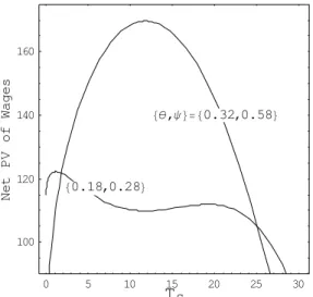
In other to calibrate the φ(TS) function we employed the speciÞcation for {θ,ψ} in Bils
and Klenow (1999). Actually, in their work there are three possible sets of parameters, and although they produce the same average return of education on wages, they differ in concavity. We employed the most concave speciÞcation. One of the reasons is that it seems to be consistent with cross-section studies of return to education. The second reason is uniqueness. TheÞrst order condition with respect to the education choice, equation (18), is:
A2 η e
φ(TS)
½
φ0(TS)
1−e−(r−g)TW
r−g −1 ¾
= 1 +τH.
Although φ(TS) is concave, eφ(TS) is convex. If there is no tuition cost (as is the case in Bils
and Klenow (1999)), the term eφ(TS) cancels out and we get local second order condition
for the solution of the Þrst order condition.21 This is not the case in our formulation. In
particular, if we considered a less concave speciÞcation for φ(TS), the observed TS for the
US would be a minimum of the calibrated net present value function, as Figure 5 illustrates. Evidently, in the distortion measurement and simulation exercises we checked whether the solution for (18) is the global maximum of the net-present-value of wages function (which has a compact domain)
B .2
U niqueness of t he calibr at ion pr ocedur e
The solution is as follows: (12) gives A2
η ; (15) and (20) giveηq; (21) givesk; and (14) (after
recalling (1)) gives A1; (18) gives τH; (14) and (21) give τK; and (17) gives ρ. It is not
possible to solve (17) explicitly for ρ. In order to get uniqueness we have to show that (17) is monotonic in ρ. That is, we have to show that
νc=f(s)≡
1−e−sT
s
s+r−g
1−e−(s+r−g)T,
where s≡g−σ(r−ρ). Calculating, we obtain
sf
0(s)
f(s) =sT[g(sT)−g((s+r−g)T)],
in which
g(a)≡ e
−a(1 +a)
−1
a(1−e−a) and g
0(a)>0.
Given that r−g >0, we have that
f0(s)<0,
which guarantees uniqueness.
B .3
I ncent ive M easur em ent
The solution is as follows. It is possible to express {τK,τH, l2, k,ηq} as a function of A1:
(21) givesk, (12) gives l2, (18) givesτH, (14) gives τK,and (15) and (20) giveηq. Then we
substitute for τK into (17), and recalling (1), we solve explicitly forA1.
R efer ences
[1] B ar r o, R and J. L ee 2000. “International Data on Educational Attainement Updates and Implications”. NBER Working Paper No. 7911.
[2] B ills, M . and P. K lenow 2000. “Does Schooling Cause Growth?,” American Eco-nomic Review, 90(5): 1160-1183.
[4] H endr icks, L . 1999. “Taxation and Long-Run Growth,” Journal of Monetary Eco-nomics 43: 411-434.
[5] Jones. C., 2002 “Sources of U.S. Economic Growth in a World of Ideas,” American Economic Review, 92: 220-239.
[6] K r ueger , A . B ., L indahl, M . 2000. “Education for Growth: Why and for Whom?” NBER Working Paper No. 7591, March.
[7] L ucas, R . 1988. “On the Mechanics of Economic Development,”Journal of Monetary Economics, 22, pp.3-42.
[8] M ankiw, N . G . 1995. “The Growth of Nations,” Brookings Papers on Economic Activity, G. Perry and W. Brainard (eds.) Washington: Brookings Institution, (1): 275-326.
[9] M at eus-P lanas, X . 2001. “Schooling and Distortion in a Vintage Capital Model,”
Review of Economic Dynamic 4: 127-158.
[10] M incer , J. 1974. Schooling, Experience, and Earning, National Bureau of Economic Research, distributed by Columbia University Press
[11] Par ent e, S. L ., Pr escot t , E. C. 1995. “Barriers to Technological Adoption and Development,” Journal of Political Economy 102: 298-321.
[12] Par ent e, S. L ., Pr escot t , E. C. 2000. Barriers to Riches, The MIT Press.
[13] Psachar opoulos, G . 1994. “Returns to Investment in Education: A Global Update,”
World Development, 22(9), pp. 1325-1343.
[14] St okey, N . L ., R ebelo, S. 1995. “Growth Effects of Flat-Rate Taxes,” Journal of Political Economy 103(3): 519-550.
[15] Tr ost el, P. A . 1993. “The Effect of Taxation on Human Capital,”Journal of Political Economy 101(2): 327-350.