Design of multidimensional compact constellations with high power efficiency

(1)

Diogo Lopes Soares

Licenciado em Ciˆencias da Engenharia Electrot´ecnica e de Computadores

Design of multidimensional compact

constellations with high power efficiency

Disserta¸cão apresentada para obten¸cão do Grau de Mestre em Engenharia Electrotécnica e de Computadores, pela Universidade Nova

de Lisboa, Faculdade de Ciˆencias e Tecnologia.

Orientador: Rui Dinis, Professor Auxiliar com Agrega¸c˜ao, FCT-UNL

Orientador: Marko Beko, Professor Auxiliar, FCT-UNL

J´uri:

Presidente: Prof. Doutor Lu´ıs de Oliveira Vogais: Prof. Doutor Rui Dinis

Prof. Doutor Marko Beko Prof. Doutor Paulo Montezuma

(2)

(3)

i

Design of multidimensional compact constellations with high power efficiency

Copyright➞Diogo Lopes Soares, Faculdade de Ciˆencias e Tecnologia, Universidade Nova de Lisboa

(4)

(5)

” At one point in your life you either have the thing you want or the reasons

why you don’t ”

(6)

(7)

Acknowledgements

Gostaria de come¸car por agradecer a ambos os meus coordenadores: Prof. Marko Beko e Prof. Rui Dinis, pela oportunidade de trabalhar neste tema e por todo o apoio, inspira¸c˜ao e disponibilidade sempre mostrada para comigo.

Para os meus pais, vai o meu maior agradecimento, pois sinto a necessidade de os destacar acima do resto: obrigado Pai e Mãe por todo o carinho, paciência, por todo o esfor¸co e por nunca desistirem de mim. Foram sem dúvida a minha maior for¸ca ao longo destes anos.

`

A minha querida avó Didi, pela educa¸cão e por todo o amor que sempre me deste, obri-gado. Ao meu irmão Francisco obrigado por seres o meu melhor amigo e pela amizade incondicional. À Raluca, obrigado por seres o grande apoio e conforto que eu encontro quando chego a casa.

Resta-me dizer que me sinto extremamente sortudo por chegar ao fim deste percurso e ver todas as amizades que fiz, todas as pessoas que acreditaram em mim e que sempre me empurraram para a frente. Um sincero obrigado a todos eles.

(8)

(9)

Sum´

ario

Cada vez mais os sistemas de comunica¸cão móveis exigem a adop¸cão de sistemas com elevados aproveitamentos de espectro e potência. Um desenho eficaz de constela¸cões de sinais apresenta-se como uma boa solu¸cão a este problema e pode significar um ganho energético bastante notório, o que diminuiria a energia total consumida pelos dispositivos. Os s´ımbolos numa constela¸cão de sinais podem ser vistos como vectores num espa¸co Eu-clidiano N-dimensional. Ao n´ıvel de uma constela¸cão com M s´ımbolos, a eficiência de potência pode ser melhorada procurando aumentar a distância entre s´ımbolos para uma dada energia de bit. Contudo, no cenário dum sistema de comunica¸cão móvel, a largura de banda apresenta-se como um factor bastante limitador.

O balan¸co entre a ocupa¸cão de espectro e a potência exigida permite encarar o desenho de constela¸cões como um problema de optimiza¸cão, mais concretamente como um problema de optimiza¸cão não convexo Quadratically Constrained Quadratic Programming.

Considerando o facto das modula¸cões empregues ao n´ıvel das comunica¸cões não serem geralmente boas em termos de eficiência de potência, nomeadamente para tamanhos de constela¸cões médio e grandes, este trabalho pretende gerar e propor novos códigos, mel-hores que os já existentes, focando o objectivo de optimizar a eficiência de potência para constela¸cões de pequena e média dimensão.

Palavras Chave: Constela¸cões multidimensionais, Eficiência de Potência, Op-timiza¸cão Convexa.

(10)

(11)

Abstract

More and more, mobile communication systems demand the adoption of high spectral and power efficiency systems. A good signal constellation design shows up as a good solution to this problem and may symbolize a remarkable energy gain, what would reduce the total devices’ energy consumption. Considering an M symbols constellation, power efficiency can be improved by increasing the distance between symbols for a given average bit energy. Symbols belonging to a constellation can be seen as vectors in an N-dimensional space. However, in a mobile communications scenario, bandwidth emerges as a very restrictive factor.

The trade-off between spectrum occupation and power requirements enables to treat the constellations design as an optimization problem, more precisely as a non convex Quadrat-ically Constrained Quadratic Programming problem.

Considering the fact that the modulations used in communications nowadays are not good in terms of power efficiency, particularly for medium and big sized constellations, this work intends to propose new codes better than the existent ones, aiming to optimize the power efficiency of small-to-medium sized constellations.

Keywords: multidimensional constellations, power efficiency, convex optimiza-tion.

(12)

(13)

Acronyms

ACG Asymptotic Code Gain

ANNN Average Number of Nearest Neighbours

APSK Amplitude-Phase Shift Keying

AWGN Additive White Gaussian Noise

BPSK Binary Phase Shift Keying

CCP Convex Concave Procedure

CDF Cumulative Distribution Function

DCP Disciplined Convex Programs

GD Gradient Descent

IB-DFE Iterative Block Decision Feedback Equalisation

ISI Intersymbol Interference

LP Linear Programs

M2_-QAM _M2_{Quadrature Amplitude Modulation}

NP Non-deterministic Polynomial-time

PAM Pulse Amplitude Modulation

PDF Probability Density Function

PSD Power Spectral Density

(14)

x

QAM Quadrature Amplitude Modulation

QCQP Quadratically Constrained Quadratic Programming

QP Quadratic Programs

SC-FDE Single-Carrier Frequency-Domain-Equalization

SDP Semidefinite Programs

SER Symbol Error Rate

SNR Signal-to-Noise Ratio

(15)

List of Figures

2.1 Conceptualized model of a digital communication system . . . 7

2.2 Model for received signal passed through an AWGN channel . . . 11

2.3 Bank of correlators . . . 12

2.4 Effect of noise perturbation on location of the received signal . . . 14

2.5 Optimal receptor . . . 15

2.6 BPSK constellation and decision regions . . . 16

2.7 Signal points for binary orthogonal signals . . . 17

2.8 Signal points for binary unipolar signals . . . 18

2.9 4-PAM signal constellation . . . 20

2.10 16-QAM signal constellation . . . 21

3.1 Feasible disposition for (N.M) = (2,12) . . . 31

3.2 Normalized constelation by a λ= 0.7 factor for (N.M) = (2,12) . . . 32

4.1 Constellation coordinates for N=5 and M=16 . . . 40

4.2 Gradient Descent constellation with M=4 . . . 42

4.7 4+12-APSK signal constellation with ρ = 2.70, r1 = 0.09014 and r2 = 0.283945 . . . 46

4.8 4+12+16-APSK signal constellation with ρ1 = 2.53, ρ2 = 4.3, r1 = 0.046, r2= 0.125 and r3= 0.2241 . . . 47

4.9 16-QAM signal constellation and its derivatives 8-QAM and 7-QAM . . . . 48

4.10 36-QAM signal constellation and its derivatives 32-QAM and 19-QAM . . . 49

4.11 Comparison of CCP, GD, APSK and QAM for M=4, M=7 and M=8 . . . . 50

4.12 Comparison of CCP, GD, APSK and QAM for M=16, M=19 and M=32 . . 50

4.13 Performance comparison of CCP and (K₋PAM)Nconstellations for (N,M)=(4,256) and (7,128) . . . 58

4.14 Performance comparison of CCP and (K₋PAM)N_{constellations for (N,M)=(6,64)} and (8,256) . . . 58

(18)

(19)

List of Tables

2.1 Values of K for different modulations . . . 24

4.1 Asymptotic Code Gain for CCP constellations . . . 41

4.2 Comparison between CCP and GD for M=4 . . . 44

4.7 Comparison between CCP and APSK for M=16 . . . 47

4.8 Comparison between CCP and APSK for M=32 . . . 47

4.9 CCP and QAM energy comparisons . . . 49

4.10 3-dimensional clusters’ energy values . . . 51

4.11 4-dimensional clusters’ energy values . . . 52

4.12 Comparison between CCP and simplex constellation for N=4 and M=4 . . 52

4.13 Comparison between CCP and simplex constellation for N=8 and M=8 . . 53

4.14 Comparison between CCP and Bi-Orthogonal Constellation for N=4 and M=8 . . . 53

4.15 Comparison between CCP and Bi-Orthogonal constellation for N=8 and M=16 . . . 53

4.16 (K₋P AM)N _{energy values . . . 54}

4.17 CCP energy values for (K₋P AM)N possible sets . . . 54

4.18 Energy of kissing number schemes by CCP . . . 56

4.19 ANNN for the generated constellations withN- number of dimensions and M - number of symbols . . . 57

(20)

(21)

List of Symbols

bi limit of constraint fi(x)

d2_ij squared distance between signal i and j

d2_min minimum squared distance

D Euclidean distance

Eb average bit energy

ES average symbol/signal energy

ei basis vector

f0(x) objective function

fi(x) constraint function

K normalized distance toD/√Eb M number of constellation symbols

M matrix of constellation vectors mi transmitted symbol

ˆ

m estimate symbol

N number of constellation dimensions

N0 Noise power spectral density

(22)

xviii LIST OF SYMBOLS

pi probability of transmitting symbol i

Pb bit error probability

Ps symbol error probability

R ratio bits per dimensions

Rw autocorrelation function of noise process w(t)

¯

s mean value of vector s

s′ _{origin centred vector}_s

si transmitted signal

T symbol time duration

vn nth component of vectorv

w(t) additive zero-mean stationary white Gaussian noise

x(t) received signal

Xj correlator’s output

C signal constellation φi(t) ith basis function

σ standard deviation

σ2

(23)

(24)

(25)

Chapter 1

Introduction

Digital communications is a wide area involving subjects from the information source until the output transducer. However, its most basic purpose involves the transmission of information under a digital form from information generative source until one or more destinations.

A great part of the transmission process is related with the transformation of the source data into some digital format in a way that information can be converted suitable to flow to the receiver through cables, fibres or through the air.

Good spectral and power efficiencies allow communications to achieve high data bit rates and to minimize the power consumption in mobile devices. It is also known that a greater spectral efficiency implies an increasing of power usage and a consequent decrease of power efficiency which is strongly undesired nowadays.

A good way to achieve a favourable trade-off between spectral and power efficiency comes from the shaping gain of a modulation. The overall gain of a transmission can be separated in two: coding gain and shaping gain. While coding gain is related with the Signal-to-Noise Ratio (SNR) levels between the coded system and the uncoded system, the shaping gain refers to the resulting reduction in signal constellation power [FHW98]. Shaping gain is strongly related with the modulation efficiency, namely the constellation design. For this reason the design of constellations with good power efficiency emerges as a good way to solve this problem.

(26)

2 CHAPTER 1. INTRODUCTION

1.1 Motivation

Presently, with the great increasing of communication devices, the limitations of spectra are more and more felt. As so, systems have to be planned and implemented to take the best of the actual resources. As a valid solution to the power efficiency problems of actual modulations, this work aims to obtain optimal constellations in terms of power efficiency. In this sense, it will be implemented a method that looks for the minimal energy cost schemes, improving the energy gains. Concretely, what is proposed is an optimization method that intends to minimize the transmit power for a given error rate, contrarily to the existent modulations that are not capitalizing the best of actual conditions.

The results sought are good solutions to implement in systems minimizing their energy consumption.

1.2 Objectives

The main goal of this dissertation is to find out good signal constellations that overcome the traditional modulations in what concerns to their energy cost. More precisely, this work looks for the minimum energy constellation that respects the minimum Euclidean distance between different constellation symbols greater or equal to 1.

The work is focused on small-to-medium sized constellations due to its more common use in actual systems, namely on a range of dimensions N from 2 _≤ N _≤ 8 and number of constellation points M where M = 2k withk= 2,3,4,5,6,7,8.

It will be presented herein a reformulation linearization-based method to find the minimum energy constellations. This practice is also known as Convex Concave Procedure (CCP). It turns the constellations design, originally formulated as a nonconvexQuadratically Con-strained Quadratic Programming(QCQP) problem, which is difficult to solve, into a convex

Second-Order Cone Programming (SOCP) problem. The SOCP problem can be solved efficiently by a convex optimization software, producing as result a new constellation with lower average symbol energy.

(27)

1.3. STRUCTURE OF THE DISSERTATION 3

1.3 Structure of the dissertation

The document is divided in 5 different chapters, as follows:

On chapter number 2, named Signal Spaces and Detection Theory, it is presented the trade-off between power efficiency and spectral efficiency in a scenario of digital com-munications; in section 2.1 there are introduced the representations of signals, with the essential definitions of orthogonality, symbol average energy and average probability of error for several modulations. The tour to a better understanding of signal constellations starts with a vector approach which enables the reader to percept the definition of signal spaces as well as Euclidean distances, fundamental to the formulation of the problem in chapter 3. Subsection 2.1.4 introduces the notion that a communication channel has to deal with noise and interference. It is followed by the receptor theory where detection is explained. In subsection 2.1.6 there are shown and compared the performances of:

Binary Phase Shift Keying (BPSK), orthogonal, unipolar binary, 16-Quadrature Ampli-tude Modulation (QAM) and N-orthogonal signal constellations. The second part of the chapter introduces high power efficient constellations, namely biorthogonal and simplex constellations.

Follows chapter 3, where the design of constellations with high power efficiency is addressed as an optimization problem. In section 3.1 some mathematical optimizations like convex optimizations and the nonconvex cases are explained and distinguished. Subsection 3.2 introduces the problem formulation under the lights of convex optimization literature. It contains the clarification of the chosen values for the problem constraints and the analysis of problem convexity. Follows the core subsection 3.3 with the proposed optimization method, explained in detail, with all the steps figuring in the algorithm and a briefly explanation of each one of them. Finally, the last section of this chapter contains an in-troduction to the Matlab’s convex optimization toolbox CVX, explaining its compatibility with the problem and the reason of its choice.

(28)

4 CHAPTER 1. INTRODUCTION

case, as well as the parameters that permit comparing the constellations. It follows the comparison of good known modulations with the proposed ones. These comparisons are first made for 2-dimensional modulations in subsection 4.3.1, where Gradient Descent,

Amplitude-Phase Shift Keying (APSK) and QAM modulations’ signal constellations are normalized and compared with the ones obtained through CCP. It follows the comparison with Sloane’s proposed clusters in 3 and 4-dimensions in subsection 4.3.2. In 4.3.3 some cases of simplex and bi-orthogonal constellations are used to evaluate the performance in cases where N=M and M=2N. Finally, multidimensional K-Pulse Amplitude Modula-tion (PAM) constellations are compared with some sets (N,M), highlighting the special importance of the comparison with some 256 symbols constellations. In section 4.3.5 it is presented some theory of the kissing number and sphere packing problems, where theoretical optimal lattices, including Voronoi constellations are compared with the ones generated by the proposed method.

(29)

Chapter 2

Signal Spaces and Detection

Theory

In what respects to real systems, severe power and bandwidth constraints are encountered. This brings the urgency of adopting power and spectral efficient systems.

The choice of the best signal constellation is not an easy task, however, setting a value for its average signal energy, here designated by ES, an optimum signal constellation is the

one that achieves a specified error probability with the lowest value of ES.

It has been proved analytically that the error probability can be made as small as desired by increasing the number of symbols in a constellation. However, what happens is that more than the increasing of receiver complexity, a bigger occupation of bandwidth is re-quired, which leads to a reduction of spectral efficiency [CC75].

This brings the need to highlight that a careful trade-off between power efficiency and spectral efficiency is required to choose the most suitable constellation for a certain sys-tem, especially in the case of multidimensional constellations, where the increase of the number of dimensions implies loss of spectral efficiency but at the same time it allows an improvement of power efficiency.

In this chapter there will be exposed some important concepts essential to judge power and spectral effectiveness of the signal sets, as well as their energy costs and gains, fundamental to a good understanding of the developed work.

(30)

6 CHAPTER 2. SIGNAL SPACES AND DETECTION THEORY

2.1 Signal Space Representations

2.1.1 A vector Analysis

Vector spaces are the subject of linear algebra and are characterized by their dimension, which specifies the number of independent directions in the space. A vector space may be characterized with additional structures, such as norm and inner product. These spaces arise naturally in mathematical analysis and abundantly in the form of infinite-dimensional function spaces whose vectors are functions.

A vectorvin ann-dimensional space is characterized by itsn components [v1v2· · ·vn]. It may also be represented as a linear combination of basis vectors ei, 1≤i≤n, as showed in equation

v= n

X

i=1

viei (2.1)

where, by definition, basis vectors have unitary length. The vector component vi is the projection of the vector v onto the unit vectorei. Thus vectorvi becomes

vi= n

X

j=1

vijej = (vi1,· · ·vin) (2.2)

One of the basic properties of vectors is the inner product, represented by a dot and denoted v1·v2. It returns a scalar value and its basic form is defined as

v1.v2 =kv1kkv2kcosθ (2.3)

where θis the measure of the angle betweenv1 and v2.

Applied to two n-dimensional vectors v1 = [v11v12· · ·v1n] andv2 = [v21v22· · ·v2n], inner

product is defined as

v1.v2 =

n

X

i=1

v1iv2i (2.4)

(31)

2.1. SIGNAL SPACE REPRESENTATIONS 7

Generally, a set of m vectorsvi, 1≤i≤m, are orthogonal if

vi.vj = 0 (2.5)

for all 1_≤i, j_≤m and i₆=j.

Other vectors’ basic property is the norm, also called length, denoted _||v_||and defined as

||v_||=p(v.v) (2.6) The squared-length of a vector is defined to be the inner product of the vector v with itself, as it can be checked on 2.6 by squaring both sides of the equation. It can also be written as the sum of the squared components of the vector

||v_||2= n

X

i=1

v_i2 (2.7)

These vectors’ properties of 2.5 and 2.6, may be used to verify if a set of vectors is

orthonormal. Clearly, a set of vectors is said to be orthonormal if the vectors besides being orthogonal also have length 1.

2.1.2 Signal spaces

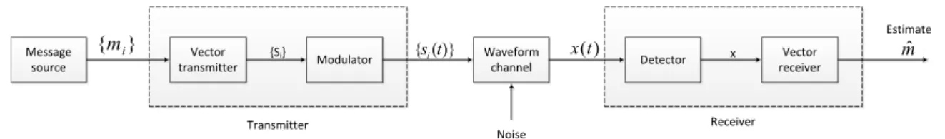
In a digital communication system, like the one in figure 2.1

Message source

Vector

transmitter Modulator

Waveform

channel Detector

Vector receiver }

{mi

Transmitter Receiver

)} ( {s_it

Noise

) (t x

{Si}

Estimate mˆ x

Figure 2.1: Conceptualized model of a digital communication system

(32)

message m=mi, the vector transmitter output takes the value

si =

        

si1

si2

.. . siN         

i= 1,2, . . . , M (2.8)

This vector si is called the signal vector and it determines the signal si(t) generated by the modulator. This is, receiving si as input, the modulator constructs a distinct signal si(t) of duration T seconds with the information from the vector.

Signalsi(t) is necessarily of finite energy 2.9

Ei=

Z T

0

s2_i(t) dt (2.9)

As it can be seen, signals have characteristics resembling vectors. Thus, it is possible to develop a parallel representation for a set of signal waveforms [Pro01].

The inner product of two general real-valued signalss1(t) ands2(t) is denoted hs1(t)s2(t)i

and it is defined as

hs1(t), s2(t)i=

Z +∞

−∞

s1(t)s2(t) dt (2.10)

Similarly to vector’s properties, signalss1(t) ands2(t) are orthogonal if their inner product

is zero.

However, the norm, assumes a much more important role in what concerns signals. Despite it is defined in the same way as the vectorial norm,

||s(t)_||=p_hs(t), s(t)_i (2.11) when considering s(t) a deterministic real-valued signal with finite energy, its squared norm represents the energy of the signal, ES.

ES =||s(t)||2 =

Z T

0

(33)

Again regarding to vector analysis, a set of orthonormal basis functionsφj(t), j= 1,2, . . . , N verifies

Z +∞

−∞

φi(t)φj(t) dt=

    

0, i₆=j 1, i=j

(2.13)

Thus, signals may be expressed as function of orthonormal basis functions φj(t) like in expression (2.14).

si(t) = N

X

j=1

sijφj(t) (2.14)

wheresiis a point in theN-dimensional Euclidean space with coordinates [si1, si2, . . . , siN]. To thisN-dimensional Euclidean space is given the name of signal space.

For what matters, a group of these signals may constitute a signal constellation _C. The energy of the ith signal is simply the square of the Euclidean distance from the origin to the point in the N-dimensional space. Thus, any signal can be represented geometrically as a point in the signal space spanned by the orthonormal functions φj(t).

2.1.3 Distances and energies

There is a close relationship between the energy content of a signal and its vectorial representation. As it was shown in (2.12) the energy of a signal si(t) of duration T is ES = R₀T s2i(t) dt. In the same manner, the energy of the signal si(t) is equal to the squared-length of the signal vector si representing it, by applying the vectorial expression (2.7).

ES = N

X

j=1

s2_ij (2.15)

In the case of a pair of signals si(t) and sk(t) whose correspondent signal vectors are si and sk, the distance between both signals is equal to the distance between both signal vectors si and sk in the Euclidean space. Thus,

dist(si,sk) =ksi−skk= N

X

j=1

(34)

Squaring both sides of (2.16), results the expression

ksi−skk2 = N

X

j=1

(sij₋skj)2 (2.17) where an interesting development is about to appear.

Looking at the properties of the vectorial norm and to the development of the square of a difference (a₋b)2 ₌_a2₊_b2₋_{2ab, the squared-distance between signals (2.17) can be}

written as

dist2(si(t), sk(t)) = N

X

j=1

s2_ij + N

X

j=1

s2_kj₋2_hsi(t), sk(t)i (2.18) which is the sum of both signals energies minus the inner product between them.

Ei+Ek−2hsi(t), sk(t)i (2.19)

In the special case where both signals are orthogonal, it was already seen that the inner product of the two signals is zero, which takes the expression (2.18) to assume the following form

dist2(si(t), sk(t)) =Ei+Ek (2.20)

In fact, this distance is called Euclidean distance, once it respects to Euclidean space. Many of energy references in formulas and expressions are showed in function of Eb,

average bit energy. The relation between Eb and ES is given by

Eb=

ES

number of bits per symbol (2.21)

The number of bits per symbol can be obtained computinglog2M, where M is the number

(35)

2.1.4 Noise

To the receiver block of figure 2.1 arrives the digital information sent by the transmitter through the transmission channel. The transmitter sends the information usingM signal waveforms si(t),i= 1,2, . . . , M. Each signal is transmitted within the symbol interval of duration T.

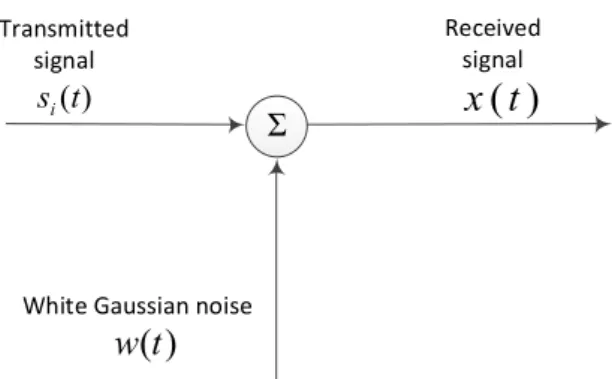
The channel however, corrupts the signal by adding white Gaussian noise, as seen in figure 2.2.

White Gaussian noise Transmitted

signal

)

(

t

w

) (t s

i

Received signal

)

(

t

x

Σ

Figure 2.2: Model for received signal passed through an AWGN channel

Thus, the received signal may be expressed as

x(t) =si(t) +w(t), 0≤t≤T , (2.22) where w(t) denotes a sample function of additive white Gaussian noise characterized by zero mean and power spectral density N0/2.

(36)

T

0

T

0 x(t)

Φ1(t)

ΦN(t)

X1

X

N

∫

Figure 2.3: Bank of correlators

Consequently, the output of each correlator is a random variableXj given by

Xj =

Z T

0

X(t)φj(t) dt

= sij +Wj, j= 1,2, . . . , N (2.23)

In (2.23), the first component, sij, is a deterministic quantity contributed by the trans-mitted signalsi(t). Although, the second component,Wj, is a random variable that arises caused by the presence of noise in the transmission channel. It is defined as

Wj =

Z T

0

W(t)φj(t) dt. (2.24)

Due to the noise’s nature, the received signalx(t) has a Gaussian distribution, what implies that the correlator’s output is also a Gaussian random variable. Hence,Xj is characterized completely by its mean value and variance.

The mean value can be discovered starting by the fact that the noise processw(t) has zero mean. Which implies that the random variable Wj obtained from (2.24) has zero mean too. Thus, the mean value of the jth correlator outputXj only depends on sij.

To find the variance of Xj, note that

σ2_X_j = Var[Xj]

(37)

Using (2.24) in (2.25), results

σ_X2_j = E

Z T

0

Z T

0

φj(t)φj(u)W(t)W(u) dtdu

=

Z T

0

Z T

0

φj(t)φj(u)RW(t, u) dt du (2.26)

where RW(t, u) is the autocorrelation function of noise process w(t).

As the noise is stationary, RW depends only on the time difference t₋u. Furthermore, the noise is also white, havingPower Spectral Density (PSD) equal to N0/2. Hence, RW

can be expressed as

RW(t, u) =N0/2δ(t−u) (2.27)

and consequently σ_X2

j comes

σ_X2_j = N0 2

Z T

0

φj(t)φj(u)δ(t−u) dt du = N0

2

Z T

0

φ2_j(t) dt

= N0

2 (2.28)

where φj(t) is an orthonormal basis.

This result shows that all correlator outputs have a variance equal to the PSD N0/2 of

the additive noise w(t).

2.1.5 Optimal receptor

When the received signal x(t) is applied to the bank of correlators depicted in figure 2.3, the correlators outputs define a new vectorx, called received vector. This received vector differs from the signal vectorsi because of the inclusion of the noise vector w.

(38)

ϕ

2

ϕ

1

ϕ

3

Observation vector

x

Signal

vector si

Message point Noise vector w Received

signal point

Figure 2.4: Effect of noise perturbation on location of the received signal

Arriving to this point, a mapping process from xhas to be performed to an estimate ˆ

m of the transmitted symbol, mi, in a way that must minimize the average probability of symbol error in the decision. The average probability of symbol error in the decision, denoted PS is

PS(mi,x) = P(mi not sent_|x)

= 1₋P(mi sent|x) (2.29)

A good detection process settles in the minimization of the distance between all the possible transmitted signal vectors [Hay88], si and the respective received vector x

min

s_i d

2₍_s_i,_x_{) = min}

s_i ksi−xk

2

= min

s_i

(Ei+Ex−2hsi,xi) (2.30) However, the expression can be simplified, dividing by two and ignoring the average bit energy of the received vector, Ex, once it is independent from the transmitted signal. Hence, (2.30) may be written as

max

s_i (hsi,xi −

Ei

(39)

where

hsi,xi=

Z T

0

[si(t) +w(t)]si(t) dt (2.32)

and

Ei =ksik2 =

Z T

0

s2_i(t) dt. (2.33)

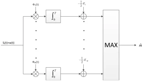
Thus, the optimal receptor can take the form presented in figure 2.5

T

0

T

0 Si(t)+w(t)

Φ1(t)

ΦM(t)

M E 2 1 1 2 1 E

MAX

mˆ

∫

−

Figure 2.5: Optimal receptor

2.1.6 Error probabilities

The model of a Gaussian distribution plays a really important role in what concerns the detection theory. As so, it is imperative to understand some concepts.

The Probability Density Function (PDF) of a Gaussian distributed random variablex is

PDF(x) = _√1 2πσe

−(x−mx)/2σ2 _(2.34)

and the Cumulative Distribution Function (CDF) of a Gaussian distributed random vari-able x is defined as

F(x) = Z x −∞ p(u) du = 1 2 1 √ π

Z (x−x¯)/√2σ

−∞

e−t2

= 1 2 +

1 2erf

x₋x¯

√

2σ

(40)

where erf(x) denotes the error function, defined as

erf(x) = √1

π

Z ∞

x

e−t2 (2.36)

For x >x¯ the complementary error function erfc(x) = √2

π

R∞

x e−t 2

is proportional to the area under the tail of a Gaussian PDF [Pro01]. Thus, it was adopted a function to denote the area under the tail of a Gaussian PDF, denotedQ(x) and defined as

Q(x) = _√1 2π

Z _∞

x

e−t2/2dt x_≥0 (2.37) 2.1.6.1 BPSK

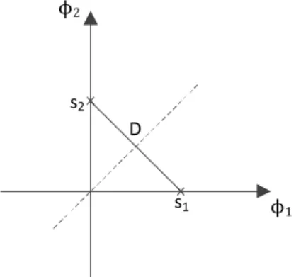
For the antipodal binary constellation represented in figure 2.6, the set of signal vectors represented are s1 =−D₂ and s2= D₂.

ϕ1

s1

s2

D 0

Figure 2.6: BPSK constellation and decision regions

Therefore, the energy of signal s1(t) can be written as E1 = D₂2 = D

2

4 . The same is

valid for s2(t), which results in average energy per bit

Eb = D2

4 (2.38)

for BPSK constellations.

The decision process relies on the choice of the transmitted signal, comparing the received signal vectorx, with the threshold zero. In casex<0, it is assumed that signals1(t) was

transmitted, in case x>0 the decision taken is that it was transmitted the signals2(t).

(41)

D/2, this is,

Pb =P

x> D 2

(2.39)

which is equivalent to

Q D/2 σw =Q s

D2_/2

N0/2

! =Q r 2Eb N0 ! (2.40)

Since signals s1(t) ands2(t) are equally likely to be transmitted, the average probability

of error is

Pb = 1

2P(e|s1) + 1

2P(e|s2) = Q r 2Eb N0 ! (2.41)

As it can be verified in relation (2.41), the probability of error only depends on the ratio Eb/N0. This ratio is called signal-to-noise ratio per bit.

2.1.6.2 Orthogonal

The type of signal constellation called orthogonal is shown in figure 2.7

ϕ2

ϕ1

D

s1

s2

Figure 2.7: Signal points for binary orthogonal signals

Here, signalss1(t) ands2(t) are orthogonal and signal vectorss1ands2are two-dimensional,

being defined as s1 =

√

Eb 0

and s2 =

0 √Eb

, where √Eb denotes the energy of each of the waveforms. Remark that the distance between both signals is D=√2Eb Assuming that signals1(t) was transmitted, the received signal vector from the correlator

is x=√

Eb+w1 w2

(42)

The probability of error is the probability that the correlation C between the received signal vector and the transmitted signal C(x,s1) is smaller than the correlation between

the received signal vector and the not transmitted signal C(x,s2). It can be expressed as

P(e_|s1) =P[C(x,s2)> C(x,s1)] =P

h

w2−w1>

p

Eb

i

(2.42)

and P w2−w1 >√Eb

returns

Pw2−w1 >

p Eb =Q r Eb N0 ! (2.43)

once w2−w1 is zero mean Gaussian with variance N0.

Due to the symmetry of the constellation, the same error probability is obtained when s2(t) is assumed to be transmitted. Consequently, the average error probability for binary

orthogonal signals is

Pb=Q

r

Eb N0

!

(2.44)

2.1.6.3 Unipolar Binary

Considering the unipolar constellation represented in figure 2.8, the set of signal vectors represented are s1 =√Eb and s2= 0.

ϕ1

s1

s2

D

0

Figure 2.8: Signal points for binary unipolar signals

Like in section 2.1.6.1, the received signal vector is

(43)

The only difference between the two modulations at this point is that the decision of what was the transmitted signal compares xwith the threshold D/2.

Assuming that the signals1(t) was transmitted, the probability of error is the probability

of x< D₂, this is

Pb =P

D/2 σn =P   s

D2_/2

N0



 (2.46)

In order to write the probability of error in terms ofEb/N0,Eb has to be calculated. So:

E1 =

N

X

j=1

s2_ij =D2 (2.47)

E2 = 0 (2.48)

Assuming that both signals are equal likely to be transmitted, the average error probability per bit is

Eb= 1 2E1+

1 2E2=

D2

2 (2.49)

Substituting Eb value in (2.46), it becomes

Pe =P

r

Eb N0

!

(2.50)

This result shows that the performance of a unipolar binary constellation is the same as an orthogonal signal constellation.

2.1.6.4 4-PAM

Figure 2.9 shows a 4-PAM signal constellation, where signals s1(t), s2(t), s3(t) and s4(t)

are represented by the signal vectors

s1 =

3 2D

(2.51)

s2 =

1 2D

(2.52)

s3 =

−1₂D

(2.53)

s4 =

−3₂D

(44)

ϕ1

s₁

s2 D

0

s3

s₄ D

D

Figure 2.9: 4-PAM signal constellation

Error probabilities are calculated considering the number of neighbours that each symbol has. In case of M-PAM constellations there are two types: the middle symbols (s2 ands3)

and the edge symbols (s1 and s4).

Assuming that signal s1(t) was transmitted, thePs is just the probability of the received vector to be in the detection range of s2(t). This is:

PS1 =Q

D/2 σw

(2.55)

The same is verified when transmitting s4(t).

In case of transmitting s2(t), errors can occur if the received vector falls either in the

detection range of s1(t) ors3(t), doubling the error probability. This implies multiplying

the previous error probability (2.55) by a factor 2, which results

PS2 = 2Q

D/2 σw

(2.56)

s3(t) verifies the same error probability.

In this signal constellation, the average energy per bit is

Eb =

E1+E2+E3+E4

(45)

while the signal energies are

E1=

9 4D

2

=E4 (2.58)

E2=

1 4D

2

=E3 (2.59)

which returns an average energy per bitEb= 10₈D2 = 5₄D2.

In case of 4-PAM, expression log2M returns 2, meaning that each symbol codifies 2 bits.

Thus,Pb results

Pb = Ps

2 (2.60)

where

PS =

PS1+PS2+PS3+PS4

4 = 3 2Q D/2 σw (2.61)

Hence, (2.60) results

Pb= 3 4Q D/2 σw = 3 4Q   s

D2_/2

N0  = 3 4Q r 4 5 Eb N0 ! (2.62) 2.1.6.5 16-QAM

Here, it will be explained the particular case of 16-QAM, however the generalization for M2₋_QAM _{constellations will be also evaluated.}

A regular 16-QAM constellation is presented in figure 2.10. The constellation is assumed to have Gray mapping.

s1 s2

s3 s4

D D

D D D

(46)

Looking at the first quadrant, there are the representations of signal vectorss1,s2,s3 and

s4 with respective coordinates in the 2-dimensional Euclidean space and signal energies:

s1 =

1 2D, 3 2D

E1 =

1 2D 2 + 3 2D 2 = 5 2D 2 _(2.63)

s2 =

3 2D, 3 2D

E2 =

3 2D 2 + 3 2D 2 = 9 2D 2 _(2.64)

s3 =

1 2D, 1 2D

E3 =

1 2D 2 + 1 2D 2 = 1 2D 2 _(2.65)

s4 =

3 2D, 1 2D

E4 =

3 2D 2 + 1 2D 2 = 5 2D 2 _(2.66)

From these values, the average energy per symbol in the first quadrant is easily obtained

ES =

E1+E2+E3+E4

4 =

5 2D

2 _(2.67)

As each symbol codifieslog2(16) = 4 bits, the average energy per bit is obtained by simply

dividingES per 4

Eb = ES

4 = 5 8D

2 _(2.68)

Note that, when transmitting signal s1(t) for instance, more than one error can occur,

which is provoked by the fact that the received signal vector can be positioned in the de-tection area of any of the 3 neighbour signals. This multiplies by a factor 3 the probability of occurring an error in the detection.

All signals are separated from their neighbours by the same distance D, which resembling to previous subsections, the probability of error considering just one neighbour is

Pe=Q

D/2 σw =Q s

D2_/4

N0/2

! =Q r 4 5 Eb N0 ! (2.69)

Although, for s1(t) the error can occur for 3 different signals, which implies

PS1 = 3Q

(47)

For the rest of the signals (of the first quadrant), their probabilities of error are

PS2 = 2Q

r 4 5 Eb N0 !

PS3 = 4Q

r 4 5 Eb N0 !

PS4 = 3Q

r 4 5 Eb N0 !

This allows the calculation of the average probability of error per symbol

PS = PS1 +PS2 +PS3 +PS4

4 = 3Q

r 4 5 Eb N0 ! (2.71)

Consequently, Pb is

Pb= 3 4Q r 4 5 Eb N0 ! (2.72) 2.1.6.6 N-Orthogonal

In the case of N orthogonal signalss1(t), s2(t), . . . , sN(t), each signal vector is represented as

s1= (α,0,0, . . . ,0)

s2= (0, α,0, . . . ,0)

sN = (0,0,0, . . . , α)

and the respective signal energies are

ES =α2 (2.73)

with

Eb = ES log2(M)

(48)

where M is the number of signals in the constellation. The distance between two orthogonal signals is

D2=_ks1−s2k2 =E1+E2 = 2α2 (2.75)

as showed in expression 2.20.

Hence, the probability of error for a N-orthogonal constellation results

Pb =Q

D/2 σw

=Q

 

s

D2_/2

N0

 =Q

r

log2(M)Eb

N0

!

(2.76)

2.1.6.7 Constellations Performance

In every error probability described along subsections 2.1.6.1 to 2.1.6.6, a factor K = D2

Eb can be verified. This factor defines the necessary energy to obtain a certain error probability. Thus, best performance constellations are those which verify the smallest factor K.

For the referred schemes, values of K are:

Constellation

Type K

Antipodal 4 Orthogonal 2

Unipolar 2

4-PAM 4₅

16-QAM 4₅

N-orthogonal 2log2(M)

Table 2.1: Values of K for different modulations

(49)

2.2. MODULATION TECHNIQUES 25

10log102 = 3dB, it leads to the conclusion that orthogonal signals are 3dB less efficient

than antipodal signals.

This difference between performances is caused by the distance between the signal points in the constellations, which is D2 = 2Eb in the case of orthogonal signals andD2 = 4Eb for antipodal signals.

2.2 Modulation Techniques

2.2.1 Multidimensional signals

When it is desired to construct signal waveforms corresponding to higher-dimensional vectors, it is possible to use either the time domain, the frequency domain or even both in order to increase the number of dimensions.

Dealing with an N-dimensional signal constellation, for any N, a time interval of length T1 =N T can be divided into N subintervals of length T =T1/N. In each subinterval of

length T, can be used binary PAM (one-dimensional) to transmit an element of the N -dimensional signal vector. Thus, the N time slots are used to transmit a N-dimensional signal.

2.2.2 Biorthogonal signals

Considering M signal waveforms sm(t), or the vector representation sm, with equal prob-ability of being transmitted. A signal set is said to be orthogonal if it is true that all M signals besides being orthogonal also have equal average energy ES values.

A set of M biorthogonal signals can be constructed from 1₂M orthogonal signals simply by adding the negative parts of each orthogonal signal. Hence, for the construction of a set of M biorthogonal signals it is required N= 1₂M dimensions.

Regarding the latter situation the minimum Euclidean distance between signals is D =

√

2ES.

2.2.3 Simplex signals

(50)

M signals by subtracting the mean from each of thesm(t) signals. Thus,s

′

m=sm−¯s, with m = 1,2, . . . , M. The effect of this subtraction is the shift of the origin sm(t) signals to the origin.

The resulting signal constellation reveals the following properties:

❼ First, the energy per signal waveform is

ks′_m_k2=_ksm−¯sk2=E− 2 ME+

1

ME =E(1− 1

M) (2.77)

❼ Second, the cross correlation of any pair of signals is

s′_m_·s′_n

||s′

m||||s′n||

=₋ 1

M₋1 (2.78)

for all m,n.

Since only the constellation’s centre of mass is translated, the distance between any pair of signal points is maintained at D, which is the same distance between any pair of or-thogonal signals. For this reason, bothPe are equal.

The expressions 2.77 and 2.78 show that a set of simplex signals is equally correlated and require less energy, by a 1₋ _M1 factor when comparing with an orthogonal signal set. Hence, simplex signalling is employed when transmission’s energy is limited.

(51)

Chapter 3

Problem Formulation and

Proposed Method

3.1 Mathematical Optimization

A mathematical optimization problem, or just optimization problem, has the form

minimize f0(x)

subject to fi(x)≤bi, i= 1, ..., m

(3.1)

Here, the vectorx= (x1, . . . , xn) is the optimization variable of the problem, the function f0 :Rn→R is the objective function, the functions fi:Rn→R, i= 1, . . . , mare the constraint functions, and the constants b1, . . . , bm are the limits for the constraints. A vector x⋆ is called optimal, or a solution of (3.1), if it has the smallest objective value among all vectors that satisfy the constraints. This is, for any z such as f1(z) ≤

b1, . . . , fm(z)≤bm, we havef0(z)≥f0(x⋆) .

3.1.1 Convex Optimization Problem

Optimization problems are divided by classes, characterized by particular forms of the objective and constraint functions. A convex optimization problem is one in which the

(52)

28 CHAPTER 3. PROBLEM FORMULATION AND PROPOSED METHOD

objective and constraint functions are convex, which means they satisfy the inequality

fi(αx+βy)_≤αfi(x) +βfi(y) (3.2) for all x,y_∈Rnand all α, β_∈R with α+β = 1, β _≥0. Equivalently, a function is said to be convex if its epigraph (the set of points on or above the graph of the function) is a convex set. There is in general no analytical formula for the solution of convex optimization problems, but there are very effective methods for solving them [BV04].

3.1.2 Non-convex Optimization Problem

On the other hand, if the objective function and/or the constraint functions are not convex, it means that the optimization problem is categorized as a non-convex optimization problem. This kind of problems is known to be hard to solve, even for a small number of constraints. However, convex optimization also plays an important role in problems that are not convex. Combining convex optimization with a local optimization method it is possible to find an approximate, but convex, formulation of the problem for the original non-convex problem. Solving this approximate problem, it is obtained the exact solution to the approximate convex problem. This point may be used as the starting point for a local optimization method, applied to the original non-convex problem. Moreover, many methods for global optimization require a cheaply computable lower bound on the optimal value of the non-convex problem. The methods for doing this are based on convex optimization.

3.1.3 Non-convex QCQPs

A non-convex QCQP can be expressed in the form:

minimize xTP0x+qT0x+r0

subject to xTPix+qTi x+ri ≤0, i= 1, ..., m

(3.3)

with variablex_∈Rn, and parameters Pi ∈Sn (Sn represents the set ofn×nmatrices),

(53)

3.2. PROBLEM FORMULATION 29

problem is convex and can be solved efficiently, otherwise the problem is a non-convex QCQP. This type of problems is Non-deterministic Polynomial-time (NP)-hard, which means that it is not straightforward to determine the complexity of the problem or respec-tive solution time, by a polynomial. Globally they are difficult to solve, once its complexity grows exponentially with the problem dimensions.

This characteristic of non-convex QCQPs leads to the need of global optimization tech-niques. These techniques are based on convex optimization and are used to find a lower bound on the optimal value of the non-convex problem.

3.2 Problem Formulation

Following what was proposed to obtain, for a given pair (N,M) the goal is to find out the minimum energy constellation _C=_{x1,x2, . . . ,xM}with xk∈RN fork= 1, . . . , M, respecting yet the constraint that the Euclidean distance between different symbols (sig-nals) must be greater or equal to a certain threshold.

This can be formulated as follows:

M=_{(x1, . . . ,xM) :kxi−xjk2 ≥D2, 1≤i < j ≤M} (3.4) where _Mis theM-sized vector ofN-dimensional vectors [BD12].

Regarding this approach, it leads to the definition of the following merit function

f :_{M →}_Rand _C=_{x1,x2, . . . ,xM} 7→f(C) as

f(_C) = M

X

i=1

kxik2 (3.5)

It is easily observed that Es = f_M(C), which means that this merit functionf(C) that was just defined is directly proportional to the symbol average energy, Es.

(54)

{x1, x2, . . . , xM}can be achieved by solving the optimization problem

C∗ = arg minf(_C)

C ∈ M,

(3.6)

or equivalently

minimize M

X

i=1

kxik2 (3.7)

subject to _kxi−xjk2 ≥D2. (3.8) Clearly, the objective function is PM

i=1kxik2 with xi ∈ RN and its constraints are the

inequalities_kxi−xjk2≥D2, with 1≤i < j ≤M.

The value of the threshold was chosen to be D= 1, once it doesn’t affect the generality of the formulation given by (3.4).

The optimization problem is classified by the convexity of its constraints [BV04]. Since all the constraints in the set M are non-convex, this optimization problem is characterized as a non-convex optimization problem. Moreover, amongst the non-convex optimization problems class, this one is a non-convex Quadratically Constrained Quadratic Program-ming.

3.3 Proposed Method

The procedure now described is often called CCP. It is a simple technique but it will be proven to be an effective mean to achieve good compact multi-dimensional constellation designs that minimize the average symbols energy for a given minimum Euclidean distance. The software used to perform the algorithm is Matlab which has also the compatibility with the convex optimization tool CVX.

Following, there are the 4 steps figuring in the written algorithm.

❼ Encounter a feasible pointx0

❼ Normalization of the constellation

(55)

3.3. PROPOSED METHOD 31

❼ CVX treatment of the SOCP

The linearization process and the calling of CVX are iterative. This means that steps 3 and 4 are executed recursively until the algorithm stops.

3.3.1 Encountering a feasible point

The first step is to randomly generate a _C constellation such as _C = _{x1,x2, . . . ,xM}, withxk∈RN fork= 1, . . . , M. This constellation has to be feasible facing the constraint (3.8), i.e., all the points of the constellation _C must have the Euclidean distance between each pair of points equal or greater than one. If (3.8) cannot be respected, it is generated a new random set of N-dimensional points and the constraint is tested again. Once the constellation obeys to the constraint, the initial feasible point is found. It has dimension [N_×M,1] and it will be designedx0 from now on.

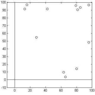
In figure 3.1 there is an example of an initial feasible point.

Figure 3.1: Feasible disposition for (N.M) = (2,12)

3.3.2 Normalization

(56)

Once the design of the optimum constellations is being done offline, the processing time is not a constraint.

What is done is simply normalize each vector xi, not with D = 1 but with a number a little bigger.

xi = xi

λ.√D (3.9)

with i= 1, . . . , M and 1

λ.√D the normalization factor/value.

In the herein study, the normalization factor is λ = 0.7, turning the minimum distance between points to be dmin ≃1.4286 in the initial disposition.

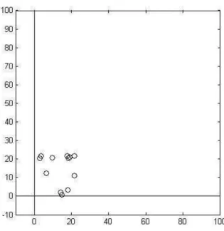
The normalization of the feasible point of 3.1 by aλ= 0.7 factor is shown in figure 3.2.

Figure 3.2: Normalized constelation by a λ= 0.7 factor for (N.M) = (2,12)

3.3.3 Linearization

The next step consists of a reformulation of the non-convex constraints, i.e., 3.8 and successive linearization around the original feasible point x0 [dB03]. Here, the convex

(57)

constraint and it is non-convex, it develops like follows:

kxi−xjk2 ≥1 (xi−xj)T.(xi−xj)≥1 (xT_i ₋xT_j).(xi−xj)≥1

xT_i xi−xTi xj−xTjxi+xTjxj ≥1, 1≤i < j≤M (3.10) Here,xi of size [N,1] similarly toxj, is defined by

xi=Ei.x (3.11)

where Ei = eTi ⊗IN. ei represents the i-th column of the identity matrix IM and ⊗ denotes the Kronecker product.

To make it easier to understand, let’s consider the case where (N, M) = (2,3).

Thus x will have the dimension [N _×M,1] and xi dimension [2,1] and Ei will be eT_i ⊗ IN, ∀1≤i≤M.

After this, obtaining x1 comes: x1 =E1.xwhereE1=eT1 ⊗I2

E1 comes

1 0 0

⊗    1 0 0 1   =   

1 0 0 0 0 0 0 1 0 0 0 0

  

and x1 will be

  

1 0 0 0 0 0 0 1 0 0 0 0

  .                 x11 x21 x31 x41 x51 x61                 =    x11 x21   

Respectively,x2 andx3 will be

(58)

Replacing in (3.10), the values ofxi and xj given by the expression (3.11), results

ET_i xT.Eix−ETi xT.Ejx−ETjxT.Eix+ETjxT.Ejx≥1

xT (ET_i Ei−ETi Ej−ETjEi+ETjEj)x≥1

xT (Eij)x≥1 (3.12) whereEij replaces the expressionETi Ei−ETiEj−ETjEi+ETj.Ej ⇔(Ei−Ej)T.(Ei−Ej). It can be now verified

kxi−xjk2≥1⇔xT (Eij)x≥1⇔

⇔1_≤xTEijx (3.13)

Thus, according to the document [dB03], where S. Boyd defines that the constraint of a general non-convex optimization problem of the format

xTP x+qTx+r _≤0 (3.14) can be rewritten as

xTP+x+qT0x+r0 ≤xTP−x (3.15)

decomposing the matrixP _∈Sninto its positive and negative parts: P =P+−P−, with P+, P−0.

Here, both sides of the inequality are convex quadratic functions, which means in advance that the non-convex QCQP problem was reformulated in order to be solvable.

(59)

is then linearized around the feasible pointx0, becoming the constraint of (3.2) of the form

1_≤xT₀Eijx0+ 2x0TEijx−2xT0Eijx0

1_≤2xT₀Eijx₋x₀TEijx0, 1≤i < j≤M (3.16)

This linearization is only possible becauseEij is semidefinite positive,Eij 0, i.e., it is a Hermitian matrix with all eigenvalues non-negative. This can be proven by its definition on equation (3.12).

Done the linearization of the constraint around x0, the problem formulation set in (3.4)

is now presented as

M⋆=_{(x1, . . . ,xM) : 1≤2xT0Eijx−xT0Eijx0, 1≤i < j ≤M} (3.17)

The right hand side of (3.16) is an affine lower bound of 1 _≤xTEijx, changing the face of the problem: it turns the feasible set of the new formulation, a convex subset of the original feasible set, resulting the constraint to be convex instead of non-convex and thus more conservative.

A new feasible point x1 can now be achieved from the convex SOCP:

minimize M

X

i=1

kxik2

subject to 2xT₀Eijx₋xT₀Eijx0 ≥1, 1≤i < j ≤M

(3.18)

3.3.4 CVX treatment of the SOCP

The convex SOCP result of the linearization, allows obtaining a new feasible point from (3.18) starting from a feasible pointx0.

The use of the convex optimization software CVX, enters here, once it can solve efficiently this type of convex problems, returning a new feasible point x1 with a lower objective

value.

(60)

that are returned by the program CVX, it is obtained a sequence of feasible points with decreasing objective values, this is, _kx1k2 ≤ kx0k2. However, the sequence doesn’t go on

indefinitely: the algorithm will stop when _kxk−xk+1k<0.001 for somek.

Remark that once the problem constraint is now convex, there is no need to keep checking if the output points belong to the feasible set of the problem: it is already implicit. Finally, the constellation’s centre of mass is shifted to the origin in order to minimize the average energy used to transmit each symbol.

3.4 Convex Optimization software - CVX

From the range of convex optimization programs and tools available to use in the project, CVX: Matlab Software for Disciplined Convex Programming, was preferred because a big part of the project’s core was based on the book [BV04, ”Convex Optimization”] from Stephen Boyd, the same author of the chosen software.

Briefly, CVX is a modeling system for constructing and solving Disciplined Convex Pro-grams (DCP). It supports a number of standard problem types, including Linear Pro-grams (LP) andQuadratic Programs (QP), SOCP, and Semidefinite Programs (SDP). It is also used to conveniently formulate and solve constrained norm minimization. CVX is implemented in Matlab, turning Matlab into an optimization modeling language. Model specifications are constructed using common Matlab operations and functions, and stan-dard Matlab code can be freely mixed with these specifications.

3.4.1 Some used commands and notions

All CVX models must be preceded by the command cvx begin and terminated with the command cvx end. All variable declarations, objective functions, and constraints should fall in between.

All variables must be declared using thevariablecommand. This command is composed by the name of the variable and an optional dimension list. For instancevariable X declares a total of 326 (scalar) variables.

(61)

3.4. CONVEX OPTIMIZATION SOFTWARE - CVX 37

(62)

(63)

Chapter 4

Numerical Results

In this chapter there will be presented the results of CCP method as well as their compar-ison with alternative modulations and/or results from other works considered good terms of comparison. These comparisons will verify the effectiveness of the proposed constella-tions.

There aren’t many documents or even algebraic or geometrical studies referencing design of constellations, lattices, clusters, etc.. sharing the work objective, specially for dimen-sions greater than 4. It doesn’t exist as well an analytic formula that features all pairs generated in terms of number of Euclidean dimensions and number of constellation points, hence these comparisons are essential to evaluate the performance of the produced con-stellations.

The present work varies its range of dimensions N from 2_≤N_≤8 and number of constel-lation points M where M = 2k withk= 2,3, . . . ,8, focusing on constellations of medium to small size.

4.1 Complexity of the method

Due to the complexity and consequent execution time of the method, the results were obtained offline and the best codes were stored. It was adopted a big number of trials in most of the cases, to obtain the best constellation’s configuration.

In the context of this dissertation, time showed to be a serious constraint. Even though, for 4-point until 64-point constellation size, there were performed 100 trials. However, for

(64)

40 CHAPTER 4. NUMERICAL RESULTS

128-point constellations the algorithm was run 20 times and 10 for 256-point ones. In an analytical approach, the procedure used to solve a SOCP convex problem, in the worst case, has complexity

O

r

1 +M(M−1) 2

(N + 1)2+ 2M(M₋1

!

(4.1)

as it is described in [PT10].

The simulation times experienced and the equation (4.1) alert to the increased difficult obtaining results on constellations with a great number of symbols. For these reasons, the range of number of constellation points present in this work isM = 2k _with_k_{= 2,}_{3, . . . ,}_8, focusing on constellations of small to medium size, mostly used in nowadays systems.

4.2 CCP constellations results

Constellations obtained are matrices like the following.

                            

3.1521 0.7201 3.5115 2.9642 3.2576 3.1046 2.1211 0.8861 2.3279 1.5350 2.2450 2.3160 2.1430 2.4791 1.9443 1.3065 3.3698 2.8533 2.8798 1.6712 1.8584 1.1869 1.0441 3.2848 0.7108 0.9940 0.2464 0.5500 2.3157 2.0943 1.8353 0.6699 1.2957 1.7506 0.2890 0.5511 2.0323 3.1873 0.5761 0.7701 3.4496 0.9650 1.1548 3.4021 0.7125 1.9294 1.3329 0.3938 2.3162 1.7405 2.3028 3.6553 3.3803 2.4817 2.8770 0.3900 2.4404 0.6968 1.2918 1.2310 0.3917 3.5592 3.6553 2.7171 2.3772 2.1926 2.9379 0.0189 3.4764 3.3231 3.2079 1.2532 3.7012 0.4667 2.5213 1.6884 1.1273 3.4973 1.9939 0.5162

                            

Figure 4.1: Constellation coordinates for N=5 and M=16

The best energy results of the new constellations are presented in figure 4.1 in order to proceed to a further comparison with equivalent schemes.

(65)

4.3. PERFORMANCE RESULTS 41

(N,M) sets that aren’t compared in the following sections, this value permits a reasonable interpretation of the constellation performance by itself.

ACG N=2 N=3 N=4 N=5 N=6 N=7 N=8

M=4 1 1.33(3) 1.33(3) 1.33(3) 1.33(3) 1.33(3) 1.33(3) M=8 0.6957 1.1344 1.5 1.5484 1.6364 1.7143 1.7143 M=16 0.4571 0.9170 1.2923 1.6 1.7010 1.8135 2 M=32 0.2817 0.6975 1.1031 1.4557 1.6928 1.8612 1.9709 M=64 0.1697 0.5213 0.8647 1.2418 1.5021 1.7678 2.0040 M=128 0.0989 0.3603 0.6911 1.0152 1.3906 1.5929 1.7918 M=256 0.0563 0.2562 0.5446 0.8498 1.1459 1.4221 1.6671

Table 4.1: Asymptotic Code Gain for CCP constellations

4.3 Performance results

This section will compare the performance of CCP constellations with benchmark schemes in use.

Remark that, in order to compare the new constellations with the existent ones, the latter ones had to be normalized with the purpose of fulfilling the minimum distance requirements: Euclidean distance between any two constellation symbols not smaller than 1.

4.3.1 Energy cost of 2-dimensional constellations

A considerable amount of literature exists on the problem of selecting an efficient set of N digital signals with in-phase and quadrature components for use in a suppressed carrier data transmission system.

The comparison with QAM, gradient descent and APSK 2-dimensional modulations is now presented, making the evaluation of the proposed method effectiveness easier.

4.3.1.1 CCP vs Gradient Descent

(66)

42 CHAPTER 4. NUMERICAL RESULTS

constellations for M=4, M=7, M=8, M=16 and M=19 points, shown next:

❼ M=4 C=    I Q   =   

1.0 1.0 ₋1.0 ₋1.0 1.0 ₋1.0 1.0 ₋1.0

  

−1.5 ₋1 ₋0.5 0 0.5 1 1.5

−1.5 −1 −0.5 0 0.5 1 1.5

GD M=4

Figure 4.2: Gradient Descent constellation with M=4 ❼ M=7 C=    I Q   =   

0.999 ₋0.855 ₋0.144 0.855 0.144 0 ₋0.999

−0.410 ₋0.660 1.070 0.660 ₋1.070 0 0.410

  

−1.5 −1 −0.5 0 0.5 1 1.5

GD M=7

(67)

4.3. PERFORMANCE RESULTS 43 ❼ M=8 C=    I Q   =   

0.624 ₋0.339 1.020 ₋0.197 ₋0.962 0.026 ₋0.603 0.431 0.946 1.082 0.065 ₋1.400 0.344 0.186 ₋0.538 ₋0.684

  

−1.5 ₋1 ₋0.5 0 0.5 1 1.5

−1.5 −1 −0.5 0 0.5 1 1.5

GD M=8

Figure 4.4: Gradient Descent constellation with M=8 ❼ M=16 C=    I Q   =   

0.007 0.126 0.644 1.279 0.906 ₋1.032 ₋0.504 ₋0.611 0.758 0.767 0.106 0.545 0.305 ₋0.771 ₋0.103 0.332 1.020 ₋0.119

     

−0.911 ₋0.388 0.245 ₋0.272 0.376 ₋1.136 0.512

−0.772 ₋0.329 ₋0.552 ₋1.001 ₋1.215 0.571 1.211

  

−1.5 ₋1 ₋0.5 0 0.5 1 1.5

−1.5 −1 −0.5 0 0.5 1 1.5

GD M=16

Design of multidimensional compact constellations with high power efficiency

Diogo Lopes Soares