Elastic scattering of protons and oxygen ions from light nuclei

(1)

Hugo Miguel Martins Ferreira da Silva

Mestre

Elastic scattering of protons and oxygen

ions from light nuclei

Dissertação para obtenção do Grau de Doutor em Engenharia Física

Orientador: João Duarte Neves Cruz, Professor Auxiliar, FCT/UNL

Júri:

Presidente: Doutora Maria Adelaide de Almeida Pedro de Jesus

Arguentes: Doutor Hans-Werner Becker

Doutor Rui Manuel Coelho da Silva

Vogais: Doutora Maria Micaela Leal da Fonseca

Doutor Eduardo Jorge da Costa Alves

(2)

ii Elastic scattering of protons and oxygen ions from light nuclei

(3)

iii

Acknowledgements

First of all, I would like to dedicate this thesis to my father. This work represents the battle of several years and I never forgot that he always wanted me to finish it. Despite all the people who I worked with in this last years, to whom I thank for their help, my special thanks go to:

To my wife, Cátia Santos Silva, for her support not only as a life mate but also as a colleague in the long runs of data taking.

Dr. João Cruz, who proposed me this Ph.D. thesis and to join the nuclear physics group.

Professor Adelaide Pedro de Jesus and Ángel Sánchez-Benítez, for their expertise in nuclear physics.

Dr. Hélio Luís, Dra. Micaela Fonseca and Dr. Daniel Galaviz for their support in experimental measurements.

To all the people of Laboratório de Aceleradores e Tecnologias da Radiação (LATR), and especially to Jorge Rocha, Filomena Baptista and Rute Pinheiro for the technical support in the implantations, evaporations and Van de Graaff accelerator operation.

Pamela Teubig, for her help with the evaporations at FCUL. Luiza Oliveira, who was always available to help.

To my family, especially to my mother, who gave me emotional support during this work, but also to my friends.

(4)

(5)

v

Resumo

Este trabalho apresenta o estudo experimental da dispersão elástica de protões e oxigénio, nomeadamente das reações 6Li(p,p)6Li, 7Li(p,p)7Li, 12C(p,p)12C, 19F(p,p)19F,

31_P(p,p)31_P,16_O(16_O,16_O)16_{O e}12_C(16_O,16_O)12_{C para o intervalo de energias de 1.6 MeV até}

3.9 MeV para a dispersão 12C(p,p)12C, 1 MeV até 2.7 MeV para a dispersão 6Li(p,p)6Li,

7_Li(p,p)7_{Li e}19_F(p,p)19_{F, 2.6 MeV até 4 MeV para a dispersão}31_P(p,p)31_{P, 8 MeV para a}

dispersão 16O(16O,16O)16O e 2.8 MeV, 5.1 MeV e 8.1 MeV para a dispersão 12C(16O,16O)12C. A dispersão elástica está sempre presente nas reações nucleares e o seu estudo fornece informação que pode ser usada para cálculos teóricos. A necessidade de valores mais precisos para as correspondentes secções eficazes dá uma motivação para a sua medição, juntamente com resultados para diferentes energias e ângulos, especialmente para a frente do plano onde ocorre a reação.

Toda a componente experimental foi desenvolvida no LATR (Laboratório de Aceleradores e Tecnologias de Radiação) do CTN-IST (Campus Tecnológico e Nuclear –

Instituto Superior Técnico) Sacavém, Portugal. Envolveu o uso da maior parte dos dispositivos experimentais do laboratório. Melhorias na configuração experimental foram feitas, quando necessárias. A preparação e caracterização de alvos foi alvo de um estudo intensivo, já que representa um desafio em experiências de física nuclear quando uma alta precisão dos resultados é necessária. Algumas das reações nucleares foram medidas com mais do que um alvo, adicionando confiança aos resultados obtidos. Foi efetuada uma comparação com cálculos teóricos, especialmente com os potenciais ópticos existentes na literatura, mostrando que estes necessitam de um ajuste, principalmente para elementos leves. Os resultados deste trabalho mostraram que a medição precisa de secções eficazes elásticas, especialmente a baixos ângulos, onde existem poucos dados disponíveis, pode fornecer informações fidedignas tanto para a obtenção de parâmetros do modelo óptico quanto para a caracterização de estados excitados nucleares.

(6)

(7)

vii

Abstract

This work presents the experimental study of elastic scattering of protons and oxygen ions, namely of the reactions 6Li(p,p)6Li, 7Li(p,p)7Li, 12C(p,p)12C, 19F(p,p)19F, 31P(p,p)31P,

16_O(16_O,16_O)16_{O and}12_C(16_O,16_O)12_{C in the energy range from 1.6 MeV to 3.9 MeV for} 12_C(p,p)12_{C scattering, 1 MeV to 2.7 MeV for} 6_Li(p,p)6_Li, 7_Li(p,p)7_{Li and} 19_F(p,p)19_F

scattering, 2.6 MeV to 4 MeV for 31P(p,p)31P scattering, 8 MeV for 16O(16O,16O)16O scattering and 2.8 MeV, 5.1 MeV and 8.1 MeV for 12C(16O,16O)12C scattering.

Elastic scattering is always present in nuclear reactions and its study gives us information that can be used for theoretical calculations. The need for more precise values for the corresponding cross sections gives a motivation for its measurement, along with the measurement at different energies and angles, especially forward ones.

The experimental work has been performed at LATR (Laboratório de Aceleradores e Tecnologias de Radiação) of CTN-IST (Campus Tecnológico e Nuclear – Instituto Superior Técnico) Sacavém, Portugal. It involved the use of the main experimental facilities of the laboratory. Improvements to the experimental setup needed for the measurements were made. Target preparation and characterization was also subject of intensive study, since it represents a struggle in nuclear experiments especially when high accuracy in measurements is required. Some of the cross sections were measured with more than one target, adding trust to the results obtained. Comparison with theoretical calculations was done, especially with the optical potential parameters available in the literature, showing that these calculations need some fine tuning, mainly for light elements. Our results showed that the accurate measurement of elastic scattering cross sections, especially at forward angles, where there is little data available, can provide reliable information both for obtaining accurate optical model parameters as well as for the characterization of excited states of nuclides.

(8)

(9)

ix

List of Figures

Figure 1.1) Linear momentum conservation in a nuclear reaction. ... 8

Figure 1.2) Particles entering the ring between b and b+db are scattered inside a ring of angular widht dθ. ... 11

Figure 1.3) The hyperbolic trajectory of a scattered particle. The change on its momentum is . ... 12

Figure 1.4) Dependence of Rutherford cross section with energy for 129Xe(p,p)129Xe ... 14

Figure 1.5) Dependence of Rutherford cross section with angle for 129Xe(p,p)129Xe. ... 14

Figure 1.6) Upper and lower limits for elastic cross section in a nuclear reaction ... 22

Figure 1.7) Dependence of and on energy. Their product is the shaded region. Effective energy (E0) in a thermonuclear reaction and its width () ... 26

Figure 1.8) Optical Model Interaction. ... 29

Figure 1.9) Calculated differential cross Section for Elab= 1.6 MeV. ... 29

Figure 2.1) Comparison of the evaluated cross section [3] and experimental data for a) θlab=110° [4,5] and b) θlab=115° [4,6]. ... 35

Figure 2.2) 12C(p,p)12C elastic cross sections measured by J.C. Armstrong et al. at θlab=65.7°, 75.4° and 85.2° [7] and comparison with theoretical evaluation [3]. ... 36

Figure 2.3) 12C(p,p)12C theoretical differential cross section at θlab=50° [9]. ... 37

Figure 2.4) 6Li(p,p)6Li experimental differential cross section for four different angles from two different authors [12,13]. ... 38

Figure 2.5) 6Li(p,p)6Li experimental differential cross section at θlab=89.5° and 90° [12,13]. ... 39

Figure 2.6) 6Li(p,p)6Li experimental differential cross section at θlab=80.5° and 81.3° [14,15]. ... 40

(14)

xiv

Figure 2.8) 7Li(p,p)7Li experimental differential cross section near 90° [19,20]. ... 42

Figure 2.9) 19F(p,p) 19F experimental differential cross section for θlab=148.52° and 150° [10,17,23]. ... 44

Figure 2.10) 19F(p,p) 19F experimental differential cross section for θlab=165°, 161.12°, 160° [10,21,23] and comparison with IBANDL theoretical calculation for θlab=160° [9]. ... 44

Figure 2.11) 19F(p,p) 19F experimental differential cross section for θlab=82.47°, 69.38° and 65.43° [22,23]. ... 45

Figure 2.12) 31P(p,p) 31P experimental differential cross section [26] and theoretical evaluation for θlab=165° [9]. ... 46

Figure 2.13) 31P(p,p) 31P experimental differential cross section for θlab=165°, 150° [25,29] and comparison with IBANDL theoretical calculation for θlab=150° [9]. ... 46

Figure 2.14 16O+16O fusion cross section for different authors [32,33,34,35,36] and theoretical models [29,37,38]. ... 48

Figure 2.15) 16O+16O total (a) and partial (b) fusion cross sections obtained with a channel coupling calculation of NRV [39]. ... 49

Figure 2.16) Ratio of 16O+16O elastic scattering cross section measured by Spinka et al. to pure Mott scattering cross section at θlab=45.0°. ... 51

Figure 2.17) Theoretical predictions for 16O+16O elastic scattering cross section. ... 51

Figure 2.18) Ratio of 16O+12O elastic scattering cross section measured by Spinka et al. to Rutherford scattering cross section. ... 52

Figure 2.19) 16O+16O and 16O+12C differential elastic cross section for Ec.m.=5 MeV. ... 53

Figure 3.1) Scheme of the 3 MV Tandem accelerator at LATR/CTN-IST. ... 59

Figure 3.2) Duoplasmatron Ion source. ... 60

Figure 3.3) a) Illustrative scheme of a stripping process in a Tandem accelerator [3].b) 3 MV Tandem Accelerator at LATR/CTN-IST ... 62

Figure 3.4) Magnetic field as a function of magnet current for the 90° analyzing magnet. ... 63

(15)

xv

Figure 3.6) Nickel plate that protects the plastic structure at the entrance of the target chamber

[4,5]. ... 64

Figure 3.7) Nickel collimator with Au evaporated [4,5]. ... 64

Figure 3.8) Upper view of the target chamber with A) Collimating system, B) Sleeve where the EG&G Ortec® GEM-45190-P HPGe detector enters, C) 2 Canberra PIPS and rotating system and D) Beam stopper. ... 66

Figure 3.9) (1) Pneumatic valve; (2) Turbomolecular pump; (3) Rotatory pump from Varian; (4) Pirani meter; (5) Penning meter; (6) Válvula manual; (7) Pneumatic valve; (8) Penning meter; (9) Turbomolecular pump from Pfeiffer; (10) Rotatory pump from Pfeiffer. ... 66

Figure 3.10) The platinum mesh of the filament after cleaning with royal water [4]. ... 67

Figure 3.11) Ressonance of reaction at ER= 872 keV. ... 68

Figure 3.12) Energy calibration of the 3 MV Tandem presented as a linear fit. ... 69

Figure 3.13) Scheme of the 2.5 MV Van de Graaff accelerator at LATR. ... 70

Figure 3.14) Tank of the Van de Graaff Accelerator at LATR. ... 71

Figure 3.15) RBS setup (line and detectors position inside the RBS chamber)... 72

Figure 3.16) Scheme of the Danfysik ion implanter at LATR/CTN. ... 72

Figure 3.17) Deceleration system: 1) Implanter target; 2) Deceleration target and 3) Lens. ... 73

Figure 4.1) Implantation profile of 16O in Ta for different nominal fluences at 70 keV. ... 79

Figure 4.2) a) Glass sheet with carbon evaporated.b) Evaporator at LATR/CTN. c) Target holder with multiple targets produced. d) Experimental apparatus for carbon evaporation. ... 80

Figure 4.3) Energy loss of the projectile ion in the target material. ... 83

Figure 4.4) (a) Experimental RBS spectra and simulation fitting performed with SIMNRA (b) Depth profile obtained from the RBS analysis. ... 84

Figure 4.5) Experimental RBS spectra and simulation fitting for 16O+59Co Implantation. ... 85

Figure 4.6) Experimental RBS spectra and simulation fitting performed with SIMNRA. ... 87

(16)

xvi

Figure 4.8) 1605 MeV H+ forward scattering spectrum measured at θlab=90°. ... 92

Figure 4.9) 2 MeV 4He+ backscattering spectrum measured at θlab=140° with a simulation

performed with SIMNRA for LiF into 12C implanted with 129Xe. ... 93 Figure 4.10) 2 MeV 4He+ backscattering spectrum measured at θlab=140° with a simulation

performed with SIMNRA for LiWO4 evaporated into 12C. ... 94

Figure 4.11) Absolute efficiency as function of energy for Ge(Hp) gamma ray detector. ... 95 Figure 4.12) Gamma ray spectrum at energy Elab=3000 keV. ... 96

Figure 4.13) 2 MeV 4He+ backscattering spectrum measured at θlab=140° with a simulation

performed with SIMNRA for Ca3(PO4)2 evaporated on self-supporting Ag. ... 97

Figure 4.14) Experimental RBS spectrum and simulation fitting performed with SIMNRA and WiNDF. ... 100 Figure 4.15) (a) Implanted and Implanted + annealed RBS spectra and (b) Depth profile obtained from the RBS analysis. ... 102 Figure 4.16) XRD spectra for the Implanted 2 and Impl. 2 + annealed targets. The arrows mark the shift induced by the thermal annealing. ... 103 Figure 4.17) RBS spectra for sputtered targets with a ratio between Argon and Oxygen of (a) 70/30 and (b) 95/5. ... 104 Figure 4.18) RBS spectra before and after the ion bombardment for the (a) Anodized, (b) Implanted and (c) Sputtered targets. ... 106 Figure 5.1) Stopping cross section of 12C for protons, , as function of energy, for the energy range from 1500 to 4000 keV. ... 114 Figure 5.2) Stopping cross section of 12C for oxygen, , as function of energy, for the energy range from 2000 to 10000 keV. ... 115

Figure 5.3) Scattering of two particles as viewed in the center of mass frame. θc is the

scattering angle in the center of mass frame (θc.m.). ... 115

Figure 5.4) Scattering of two particles as viewed in the laboratory frame. θ is the scattering angle in the laboratory frame (θlab). ... 115

Figure 5.5) Yield of Xe as a function of energy for θlab=90°. The red curve represents the

(17)

xvii

Figure 5.6) Yield of Xe as a function of angle for Elab=1621 keV. The black curve represents

the angular dependence of Rutherford´s formula. ... 119

Figure 5.7)The 1610 keV H+forward spectrum for target 1 at θlab=90°. ... 120

Figure 5.8)The 1610 keV H+forward spectrum for target 2 at θlab=90°. ... 120

Figure 5.9) 12C(p,p)12C differential cross section for θlab=90°. ... 120

Figure 5.10) Resonance region in 12C(p,p)12C differential cross section for θlab=90.0°. ... 121

Figure 5.11) a) Resonance fitting for target 1 using equations 5.16 and 5.18 and b) Resonance fitting for target 1 using equations 5.4 and 5.18. ... 123

Figure 5.12) a) Resonance fitting for target 2 using equations 5.16 and 5.18 and b) Resonance fitting for target 2 using equations 5.4 and 5.18. ... 123

Figure 5.13) 12C(p,p)12C differential cross section for θlab=77.7°. ... 124

Figure 5.15) 12C(p,p)12C differential cross section for θlab=67.7° and θlab=67.3°. ... 125

Figure 5.18) 12C(p,p)12C differential cross section for θlab=45.0 °. ... 126

Figure 5.19) 13N nuclear level scheme. ... 127

Figure 5.20) a) Comparison between 12C(p,p)12C differential cross section for θlab=67.3° (present work) and θlab=65.7° (J. C. Armstrong [10]) and b) Comparison between 12C(p,p)12C differential cross section for θlab=77.7° (present work) and θlab=75.4° (J. C. Armstrong [10]). ... 128

Figure 5.21) NRV simulation using A. Gurbich optical model parameters and NRV fitting for a) 1606 keV b) 2496 keV and c) 2991 keV. ... 130

Figure 5.22) a) Re( ) as function of orbital angular momentum and b) Im( ) as function of orbital angular momentum . ... 131

Figure 5.23) The 1596 keV H+forward spectrum for LiF target at θlab=90°. ... 133

Figure 5.24) The 1592 keV H+forward spectrum for LiCl target at θlab=90°... 133

(18)

xviii

Figure 5.26) 6Li(p,p)6Li differential cross section for θlab=90.0°. ... 134

Figure 5.27) 7Be nuclear level scheme. ... 134

Figure 5.28) Resonance region of the 7Li(p,p)7Li differential cross section at θlab=69.5° fitted with a gaussian function. ... 135

Figure 5.29) 6Li(p,p)6Li differential cross section for present work for θlab=90.0° and comparison with previous works [16,17] for θlab=81.3° and θlab=80.5°. ... 136

Figure 5.30) 6Li(p,p)6Li differential cross section for present work for θlab=90.0° and comparison with previous works [18,19]. ... 136

Figure 5.31)7Li(p,p)7Li differential cross section for present work for θlab=69.5°. ... 137

Figure 5.32) 7Li(p,p)7Li differential cross section for present work for θlab=90.0°. ... 138

Figure 5.33) 7Li(p,p)7Li differential cross section for present work and comparison with the work from P.R. Malmberg [20] for θlab=90.0°. ... 138

Figure 5.34) 7Li(p,p)7Li angular distributions for Eeff=1596 keV. ... 139

Figure 5.45)Ratio to Rutherford cross section for the six angular distributions for the LiF target. ... 141

Figure 5.46) a) Experimental and theoretical differential cross section for Eeff=2588 keV and b) Experimental and theoretical ratio to Rutherford cross section for Eeff=2588 keV.. ... 141

(19)

xix

Figure 5.48) Ratio to Rutherford cross section for θlab=69.5°... 143

Figure 5.49) 19F(p,p)19F differential cross section for θlab=90.0°. ... 144

Figure 5.50) Ratio to Rutherford cross section for θlab=90.0°... 144

Figure 5.51) a) Comparison between 19F(p,p)19F differential cross section for θlab=69.5° (present work) and θlab=69.38° (S. Ouichaoui et al. [21]). ... 145

Figure 5.52) 19F(p,p)19F angular distributions for Eeff=1596 keV. ... 145

Figure 5.58) a) Experimental and theoretical differential cross section for Eeff=1596 keV and b) Experimental and theoretical differential cross section for Eeff=1794 keV. ... 147

Figure 5.59) a) Scattering matrix elements for Eeff=1596 keV ans b) Scattering matrix elements for Eeff=1794 keV. ... 147

Figure 5.60) dependence for protons scattered from Ag, as function of energy. ... 148

Figure 5.61) The 3735 keV H+ backscattering spectrum at θlab=155.0°. ... 149

Figure 5.62) 31P(p,p)31P differential cross section for θlab=155.0°. ... 149

Figure 5.63) 31P(p,p)31P differential cross section of present work and comparison with previous works in the same energy range [22,23]. ... 150

Figure 5.64) Current intensity of multiple charge states for oxygen for 1600 kV. ... 151

Figure 5.67) Elastic reaction spectrum for 8 MeV of 16O3+for θlab=45°. ... 153

Figure 5.68) Elastic spectrum for 8086 keV of 16O5+for θlab=39.5°. ... 155

Figure 5.69) 129Xe angular dependence on Rutherford formula for Elab=2783 keV. ... 156

(20)

xx

Figure 5.71) 12C(16O,16O)12C elastic cross section for Elab=2783 keV, Elab=5087 keV and

Elab=8087 keV. ... 157

Figure 5.72) 12C(16O,16O)12C recoil cross section for Elab=2783 keV, Elab=5087 keV and

(21)

xxi

List of Tables

Table 1.1) Default Optical Model parameters for p+12C elastic cross section. ... 29 Table 2.1) Branching ratios for different exit channels in 16O+16O fusion reaction. ... 49 Table 3.1) 90° Analysing Magnet current values as a function of charge state and terminal voltage for 1H and 16O. ... 63 Table 3.2) Comparison between theoretical and experimental values for the resonances

measured at E50%. ... 70

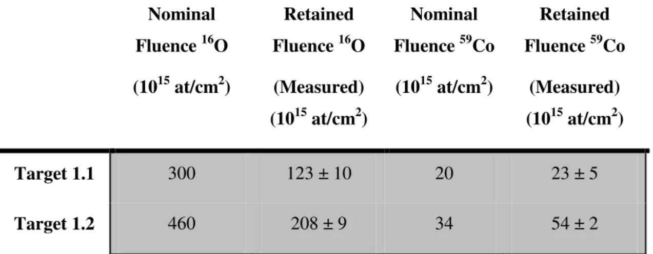
Table 4.1) Concentrations of Co, Fe and Zn given by RBS and PIXE. ... 85 Table 4.2) Retained fluence (measured) vs Nominal fluence in the implanted targets. ... 86 Table 4.3) Retained fluence (measured) vs Nominal fluence in 7Li implanted targets in Al and C. ... 91 Table 4.4) Retained fluence (measured and predicted) vs Nominal fluence in the implanted targets. ... 101 Table 4.5) Thickness, atomic abundance and Ta/O ratio in the oxide layer for the sputtered targets. ... 104 Table 5.1) Optical model parameters used in the NRV code simulations. ... 129 Table B.1) 12C(p,p)12C differential cross section for θlab=45.0°……….173

Table B.2) 12C(p,p)12C differential cross section for θlab=55.0°……….174

Table B.9) 12C(p,p)12C differential cross section for θlab=90.0°. ………...181

Table B.10) 6Li(p,p)6Li differential cross section for θlab=69.5°………182

(22)

xxii

Table B.19) 19F(p,p)19F differential cross section for θlab=69.5°………190

Table B.20) 19F(p,p)19F differential cross section for θlab=90.0°………191

Table B.21) 31P(p,p)31P differential cross section for θlab=155.0°………..192

(23)

xxiii

List of symbols

Diffuseness parameter

Magnetic field

Backscattered fraction ions Impact parameter

Speed of light

Minimum distance of approach

Differential cross section Retained fluence

Nominal fluence

Center-of-mass reference frame energy Laboratory reference frame energy Effective energy

Incident energy

Effective (Gamow) energy

Energy of the excited state

Resonance energy Electric charge

Fraction of incident particles

Scattering amplitude FC Faraday Cup

Gamow factor Planck constant

(24)

xxiv

Current density Wave number

Bolztmann constant Kinematic factor

Orbital angular momentum Magnetic quantum number Mass

Substrate atomic density

Particles distribution

Areal density (number of particles per square centimeter) Number of incident particles

Number of interactions

Linear momentum vector Particle density

Legendre polynomial Charge state

Reaction Q-value Coulomb radius Projected range Radius

Position vector

Angular distribution

Sputtering yield S-matrix

(25)

xxv

Kinetic energy

Absolute temperature in billions of K Uncertainty

Velocity vector

Effective potential Coulomb potential

Real component of volume central Imaginary component of volume central Width

Depth

Reaction yield per incident particle Atomic number

Resonance width Kronecker delta

Phase shift

Target thickness

Beam energy distribution

Width of Gamow energy distribution

Straggling

Permittivity of free space Stopping power cross section

Effective stopping power cross section

Sommerfeld parameter

Scattering angle in center-of-mass frame Scattering angle in laboratory frame

(26)

xxvi

Parity Density

Reaction cross section Coulomb phase shift Azimuthal angle Wave function

Total wave function

Solid angle in laboratory frame

(27)

xxvii

List of acronyms

AMS Accelerator Mass Spectrometry CTN Campus Tecnológico e Nuclear EBS Elastic Backscattering Spectrometry FWHM Full Width at Half Maximum IBA Ion Beam Analysis

IBANDL Ion Beam Analysis Nuclear Data Library IST Instituto Superior Técnico

LATR Laboratório de Aceleradores e Tecnologias de Radiação NRA Nuclear Reaction Analysis

NRV Nuclear Reactions Video Project PIGE Particle Induced Gamma-ray Emission PIPS Passivated Implanted Planar Silicon PIXE Particle Induced X-ray Emission

(28)

1

Introduction

In nuclear physics, experiments must be combined with theoretical evaluations to study the interaction´s potential between the projectile and target due to nuclear forces. Among all the information which can be taken from those interactions, elastic scattering has an essential role, not only because it is always present in nuclear reactions, but also because it gives important information both for experimentalists and for theoreticians.

Elastic scattering occurs when there is no excitation of internal degrees of freedom of the particles in a collision process or when the sum of the kinetic energies of the colliding particles remains constant [1,2,3]. The Rutherford scattering is an example of elastic scattering that is only valid when the scattering is induced by a pure coulomb field. When the distance between the particles interacting in the collision is too small, we should take into account the nuclear forces. By the study of elastic scattering processes it is possible to get information about the interaction´s potential between the projectile and target due to nuclear forces. The goal is to obtain the effective potential from the angular distributions of scattered particles measured experimentally. That is the reason why the elastic scattering processes are so important in nuclear and particle physics. From the analytical point of view, the measurement of elastic scattering cross sections is applied to the characterization of materials using Ion Beam Analysis (IBA), which rely on the available data and its accuracy cannot exceed that of the available cross sections [4,5].

(29)

2

In this work, the elastic scattering of protons and oxygen ions has been studied. For this, a special care was taken with experimental setup development. Additionally, an exhaustive target production and characterization has been carried out, since it is one of the most important tasks in nuclear physics experiments. For protons, 6Li(p,p)6Li, 7Li(p,p)7Li,

12_C(p,p)12_C,19_F(p,p)19_{F and}31_P(p,p)31_{P differential cross sections were measured and the}

results were compared with previous data and theoretical evaluations available, when possible. 12C(p,p)12C was the benchmark reaction for this study, providing us reliability in our experimental results for the other elements. These results will be available for the scientific community both for material analysis and theoretical calculations. Concerning the elastic scattering with oxygen ions, the purpose was to start the work with heavy ions in our laboratory, preparing the setup for future measurements. Reaction of oxygen ions with 1H, 12C and 16O were studied and data was compared with expected values.

(30)

3

References

[1] K. Krane, Introductory Nuclear Physics, John Wiley & Sons, 1988. [2] C. Iliadis, Nuclear Physics of Stars, Wiley-VCH, 2007.

[3] C. Fiolhais, R. Marques, Física Nuclear, Fundação Calouste Gulbenkian, 1993. [4] A.F. Gurbich, Nucl. Intr. and Meth. B 268 (2010) 1703.

[5] J.A. Leavitt, L.C. McIntyre Jr., M.R. Weller, in: J.R. Tesmer, M. Nastasi (Eds.), Handbook of Modern Ion Beam Analysis, MRS, Pittsburgh, PA, 1995.

(31)

(32)

5

Chapter 1 -

Nuclear Reactions

(33)

6

1.1 Introduction

When particles coming from an accelerator, reactor or a radioactive source hit a target there is the possibility that a nuclear reaction takes place [1]. In this chapter, we will describe the types of reactions and conservation laws, the energetics of nuclear reactions before entering in the discussion of nuclear reactions cross section and present the equations necessary to calculate it.

1.2 Types of reactions and conservation laws

Typically, a nuclear reaction is designated by , where a is the accelerated projectile, X is the target, b and Y are the reaction products. Sometimes, the same reaction can be presented in a compact way X(a,b)Y, which will be seen in this thesis. By definition, the Q-value is given by:

1.1

where is the mass of each particle and is the speed of light in vaccum.

There are many ways to classify the nuclear reactions. If the incident and outgoing particles are the same, it is an elastic scattering process if the products are in the ground states or inelastic scattering process if one of the products is in the excited state. In this work, we will focus in the elastic scattering process and how to measure the nuclear reaction rates.

- Elastic scattering : ;

;

(34)

7 - Inelastic scattering :

;

where is the energy of the excited state .

Considering the interaction process, we can identify two opposites: direct reactions and compound nucleus reactions. In direct reactions, the reaction proceeds in one step:

. In this case, only few nucleons take part in the reaction with the remaining nucleons of the targets being only spectators. In compound nucleus reactions, the incoming particle and the target nuclei briefly share the energy before the outgoing nucleon is ejected. In this case, we have . When the cross section dependence on projectile energy shows resonances, the energy available matches an excited state of the compound nucleus for that reaction.

1.3 Energetics of nuclear reactions

The conservation of the total energy in a typical nuclear reaction gives us:

1.2

where are kinetic energies (for which we can use the nonrelativistic approximation at low energies) and are rest masses.

The Q-value is the same as the excess of kinetic energy of the products:

1.3

The changes in mass and kinetic energy must be related to the expression of special relativity , where any variation in kinetic energy of the particles system must be balanced by the same variation in rest energy.

(35)

8

particles, then conservation of the component of the momentum perpendicular to the plane implies that the second particle must lie in the same plane as well.

Conservation of the linear momentum along and perpendicular to the beam direction gives us (figure 1.1):

1.4a

1.4b

Figure 1.1) Linear momentum conservation in a nuclear reaction.

The three last equations gives us a system of three equations and four unknowns ( ,, e ), if and are known quantities and therefore is a parameter that can be controlled. This system has no unique solution.

As usually we don´t observe the particle , it is possible to eliminate and from the equations and find a relation between and . After some algebra (see Appendix A.1 for details), is obtained:

(36)

9

There is an absolute minimum value of below which the reaction is not possible. This happens when and it is called threshold energy :

1.6

If , there is no condition for which the reaction does not occur.

A double value situation for in equation 1.5 occurs for energies between and the upper limit:

1.7

This situation also occurs only when and and is important for reactions involving nuclei with comparable masses.

1.4 Reaction Cross Section

The cross section is a measure of the probability of a given reaction to occur [1,2,3]. A beam of (particles per unit time) is entering the nuclear chamber and if the number of target nuclei is per unit area and considering the reaction cross section to be , the number of interactions per unit time is given by:

1.8

The units of reactions cross sections are units of area, cm2 or more frequently barns ( _).

If a detector is placed in a direction with respect to the beam direction, the detector defines a small solid angle at the target and can´t detect all outgoing particles. Thus, only a small fraction is taken into account and therefore only a small fraction of the cross section is measured.

(37)

10

Moreover, the outgoing particles will not in general be emitted isotropically, but they will have an angular distribution that will depend on and possibly on . If this angular distribution function is represented by a function (), we will have that

. Then

1.10

The quantity is called differential cross section and its measure gives us important information about the angular distribution of the reaction products. Knowing that the solid angle is measured in steradian, the unit for the differential cross section is barns/steradian. The reaction cross section can be calculated by integrating over all angles. With the substitution , we have that:

1.11

If is constant, the integral gives us that .

1.5 Coulomb Scattering

Coulomb scattering is the electrostatic scattering of a beam of charged particles, due to the fact that the nucleus is electrically charged. This scattering can be either elastic or inelastic.

The elastic Coulomb scattering is also called Rutherford scattering in tribute to Ernest Rutherford, who discovered the nucleus from his experiences with alpha particles.

(38)

11

At intermediary points in the trajectory, the energy is partly kinetic and partly potential and the conservation law gives us for any impact parameter:

1.12

where is the velocity, is the charge of the projectile, is the charge of the target and is the permittivity of free space.

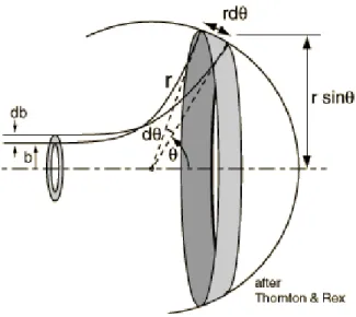
Figure 1.2) Particles entering the ring between b and b+db are scattered inside a ring of angular widht

dθ.

This scattering has cylindrical symmetry about the beam axis due to the symmetry of Coulomb force and the differential cross section becomes independent from the azimuthal angle . Particles with impact parameter between and are scattered inside the ring with angles between and , as we can see in figure 1.2. If the target nucleus has nuclei per unit area, assuming that the target is thin enough not to occur a shadow effect of a nucleus by another, the fraction of incident particles which pass through the ring is:

1.13

The fraction for impact parameters less than is:

(39)

12

Figure 1.3) The hyperbolic trajectory of a scattered particle. The change on its momentum is .

The linear momentum of scattered particles changes only in direction (figure 1.3). Far from the scattering, the initial and final linear momentum is (assuming that the target is so heavy that stays at rest. The change in the momentum is a vector of magnitude (see Appendix A.2):

1.15

According with Newton´s second law in the form , this is equal to the Coulomb force in that same direction:

1.16

where is the angle between the bisector and the instantaneous vector locating the particle. In the initial position, far from the scattering (), the angle takes the value _–

; in the final position ( ), the angle takes the value .

The instantaneous velocity can be written as function of its radial and tangential components:

1.17

where e are unit vectors in the radial and tangential directions, respectively. Only the tangential direction contributes to the angular momentum relative to the nucleus:

(40)

13

Far from the nucleus, the angular momentum takes the value , thus the angular momentum conservation gives us that:

1.19

Replacing it in the linear momentum variation equation:

–

1.20

Therefore, the conservation of the linear momentum, angular momentum and energy, imply the following relation between the scattering angle and the impact parameter :

1.21

where is the distance of closest approach.

Reminding that , we have:

1.22

and the rate at which particles reach the ring, per solid angle unit, is given by:

1.23

With for an axial geometry ( ), we have:

1.24

(41)

14 800 1200 1600 2000 2400 2800 3200

0 10000 20000 30000 40000 129 Xe(p,p)129 Xe 1/Ta 2 Dependence =70.0° D if ferent ial c ros s s ec tion / m b. s r -1

Energy / keV

30 60 90 120 150

20000 40000 60000 80000 129 Xe(p,p)129 Xe 1/sen4 (

c.m./2) dependence

T

a=2000 keV

D if ferent ial c ros s s ec tion / m b. s r -1

_c.m. / °

Figure 1.4) Dependence of Rutherford cross section with energy for 129_Xe(p,p)129_Xe

Figure 1.5) Dependence of Rutherford cross section with angle for 129_Xe(p,p)129_Xe.

To take into account relativistic effects, Rutherford cross section modifies to Mott cross section [4,5], given by:

1.25 where , being the velocity and the speed of light.

The Rutherford cross section presented was deduced taking into account the classical formalism. The same result can be obtained by solving the Schrödinger equation (see below) for a point-Coulomb potential [6].

1.6 Elastic Scattering

(42)

15

treated using the center-of-mass coordinates considering the scattering of only one particle with reduced mass by a force located in the center-of-mass.

One of the problems describing nucleon-nucleon interaction is the absence of knowledge of the fundamental strong interaction, so approximations are needed. The use an effective potential is applied instead of the calculation of all nucleon-nucleon interactions [3]. These effective potentials are deduced for specific reaction and energies; so they are not general. They depend on the magnitude of the radius vector, but not on its direction,

, where .

The theoretical treatment of elastic scattering involves solutions of the time dependent Schrödinger equation or the scattering of wave packets, which consists in solving scattering problems by decomposing each wave into its constituent angular momentum components and solving using boundary conditions but the more important physics aspects can be derived using the stationary problem of the time-independent Schrödinger equation, which is:

1.26

where is the energy.

The total wave function can be expressed by the sum of two stationary waves, an incoming plane wave and an outgoing spherical wave:

1.27

where is the incoming wave traveling in the z-direction (free particle), so and represents the spherical wave where is the scattering amplitude and the factor shows the dependence with the inverse square law. is a overall normalization factor.

The particle density (in units of inverse volume) is given by and the current density (in units of inverse area per time) of beam particles is given by . For the incoming wave, we have:

_1.28

(43)

16 1.29

The differential cross section is given by , since for elastic scattering we have that . This result shows that the differential cross section is equal to the square of the scattering amplitude. This result could also be deduced from the quantum expression for the current density:

1.30

The specific problem is the calculation of the scattering amplitude for a given potential. Once knowing this, the differential cross section is easily calculated as shown before. In the elastic scattering process, for each impact parameter there is a scattering angle

θ.

Usually, we first consider the problem using a force-free particle. The plane wave

_{represents a free particle of momentum}_{and energy given by}

. As the

potential is , the scattering amplitude is also . As said before, the plane wave can also be given by _{if we choose the z axis along}_{. Since}_{, we only}

need to consider values of for the magnetic quantum number. The spherical harmonics (see Appendix A.3) for this case are given by:

1.31

where is a Legendre polynomial. With the substitutions

and , the radial equation for a free particle can

be written as

. The solutions are called spherical Bessel functions and it is possible to write for the asymptotic values:

_, 1.32

(44)

17

1.33

The plane wave with orbital angular momentum has been expanded into a set of partial waves, each having an orbital angular momentum , an amplitude of and a phase factor . For very large distances appropriate for any experimental detector geometry, we find for a free particle:

,

1.34

If we take into account the relationship we can write

,

1.35

For the special case of s-waves in which , we have instead of equation 1.32. For this case, the equations 1.34 and 1.35 are not only valid for , but apply to all distances.

For a central potential ( and therefore ), the only difference is in the radial equation, that will change. The will change for that differ just for small where . For large distances and the two functions satisfy the same radial equation.

, 1.36

The only difference between this wave function and the radial wave function for a free particle is the phase shift that contains the dependence in the region where . For s-waves () the equation 1.36 applies to all the distances outside the potential.

Now, it´s possible to write the total wave function as a sum of partial waves:

1.37

(45)

18

,

1.38

Using the relation _{the total wave function can be written as:}

,

1.39

The difference between this wave function and the total wave function for a free particle is that the potential modifies at large distances each outgoing spherical wave by a factor ( matrix) and thereby shifts each outgoing spherical wave by a phase .

The solutions for the scattering amplitude can be achieved by writing

1.40

Knowing that and that _gives:

1.41

The introduction of a scattering potential shifts the phase of each outgoing partial wave, so the differential cross section can be written as:

1.42

For each value of , the function translates into a specific angular distribution. Concerning this, we can use the orthogonality relation for Legendre polynomials

1.43

(46)

19

1.44

Again, for the cases where we find

1.45

These results show that the angular distribution becomes isotropic (independent of ). The cross section is determined by the phase shift , which approaches 0 when the potential

for all .

These results are obtained assuming that at least one of the particles is uncharged. If both particles are charged, the phase must be replaced by , which takes into account short-range nuclear potential and the long-range Coulomb potential. So,

_1.46

Thus, the scattering amplitude can be described by:

1.47

The first term of the equation describes the contribution of the Coulomb field for the scattering amplitude (Rutherford scattering). As the second term contains both phase shifts

, the cross section will be dependent on both nuclear and Coulomb potential. The differential cross section can be given by [7]:

1.48

(47)

20

go to zero for large . This series only has meaning if a screened Coulomb potential is used, and then the radius let tend to infinity. In this case, the Coulomb scattering amplitude was found to be [6,7]:

1.49

where is called the Sommerfeld parameter.

Of course, elastic scattering is not the only process occurring between two particles. Particle capture, inelastic scattering or even fusion can occur. Different channels correspond to a specific set of conditions for the outgoing particle.

If elastic scattering is the only possible process, the number of incoming particles is equal to the number of outgoing particles surrounding the target nucleus. Concerning this, the integral over the current density , corresponding to the total wave function is zero

1.50

If there are other nonelastic processes occurring, a fraction of the incoming particles will change their kinetic energies (inelastic scattering) or change identity (particle capture). A defined number of the incoming particles will disappear and there will be a net current of particles into the imaginary sphere. This disappearance from the elastic channel corresponds to the reaction cross section.

1.51

The total wave function corresponding to a current density is the total wave function for elastic scattering. It is important to relate the reaction cross section to the phase shifts. The quantum mechanical expression for the current density was presented in equation 1.30.

For the incoming plane wave we have:

1.52

(48)

21

1.53

Applying the orthogonality relation for Legendre polynomials (equation 1.43) we get:

1.54

where in order to . Usually the phase shift is a complex number, where . If is real we have _{=1. It means that the only process}

occurring is the elastic scattering.

We can find a maximum at , where , and . The maximum reaction cross section is obtained when , having

.

(49)

22 Figure 1.6) Upper and lower limits for elastic cross section in a nuclear reaction.

The theory of scattering has been used for studying the nuclear potential. The differential cross section is obtained by experiment and used to find the potential

(50)

23

1.7 The Optical Model

The interaction potential between a nucleon and a spherical nucleus is usually described by an attractive nuclear well of depth with radius slightly larger than the nuclear radius, and a diffuse nuclear surface ( ), being the distance between the center of mass of the two nuclei [6]. The nuclear scattering is treated in similar form as the scattering of light by a glass sphere and the name of the model derives of this analogy. Most commonly we have the Woods-Saxon shape:

1.55

Usually, the central depth is about 50 MeV and the diffuseness is about 0.6 fm. The radius is proportional to the size of the nucleus and commonly around for a nucleus with nucleons where is approximately 1.2 fm. When the interaction is between two nuclei with mass numbers and , we have .

Charged particles experience also a Coulomb potential. If the charge is uniformly distributed over a radius of for a nucleus of nucleons, then for a incident nucleon of charge , the Coulomb contribution is given by:

1.56

The nuclear and Coulomb potentials are usually combined with an imaginary term and a spin-orbit part. The imaginary term, which takes into account the absorption effects (including inelastic scattering), is also often described by a Woods-Saxon form:

1.57

(51)

24

All the parameters (depth, radii and diffuseness) should come from some model or by fitting the elastic scattering angular distributions. Usually the radii for the imaginary parts are slightly larger than the real radii, reflecting that the absorption occurs from direct reaction just at and outside the nuclear surface.

The phenomenological optical model parameters for a nucleon-nucleus scattering,

, is defined as:

1.58

where is the Coulomb potential, and are the real and imaginary components of the volume-central (), surface-central () and spin-orbit () potentials, respectively. , and have been defined from equations 1.55 to 1.57. The other terms are given by:

1.59

where is the Woods-Saxon form factor and is the pion mass.

is responsible for the absorption in the whole volume of the nucleus, but

(52)

25

1.8 Model Calculations for

16

O+

16

O Elastic and Fusion

Reaction

In a stellar environment, the reacting particles (a+X) are described by a Maxwell-Boltzmann distribution:

1.60

where is the center of mass energy, is the temperature and is the Stefan-Bolztmann constant.

The cross section is related to:

1.61

where G is the Gamow factor and is given by:

1.62

1.63

where is the reduced Planck constant, is the relative velocity, and present the atomic number of the interacting nuclei, the permitivity of free space and is the reduced mass. The energy is given in MeV.

(53)

26

Figure 1.7) Dependence of and on energy. Their product is the shaded region. Effective

energy (E0) in a thermonuclear reaction and its width ()

The reaction rate depends on the product and the number of particles available at a specific energy:

1.64

which is the shaded region in figure 1.7. The effective energy (Gamow energy) and width of the distribution, , are given by:

1.65

1.66

The nuclear reactions in stars must be studied in energies of , not at energies of . The equation 1.61 can be written:

1.67

(54)

27

In massive stars, at an advanced stage of stellar evolution, the gravitational collapse increases the core temperature and density and ignites the carbon and oxygen burning (a process that strongly depends on the mass of the star). The fusion reaction 16O+16O is essential for understanding the nuclides burning processes in such advanced stages of stellar evolution, contributing significantly to the production of heavier elements. The temperature ranges from , and temporal scales from seconds

to years.The effective energy, , being the absolute temperature in billions of K, ranges from 3.9 MeV até 9.8 MeV [8]. The nuclear study of this reaction of astrophysical interest includes the measurement of both elastic and fusion cross section.

The first trial to understand the general trend of heavy-ion fusion reactions was carried out by Stokstad et al. [9], which used a strong-absorption optical potential with ,

, and over a 6 MeV range around the interaction barrier, for nine pairs of heavy ions reactions. The parameters are those from Woods-Saxon potential

1.68

Good agreement with energy dependence for all systems was obtained, except for

16_O+16_{O reaction. Adding to this, to a different excitation function, the absolute measured}

cross section was nearly a factor of 2 higher than the calculated value.

After this, Christensen and Switkowski [10] used the Incoming Wave Boundary Condition to fit elastic and fusion cross sections for the reactions 12C+12C, 12C+16O and

16_O+16_{O. For each reaction, the model parameters were determined by fitting the experimental}

elastic scattering data and the same set of parameters were used to fit the fusion data. Good agreement was obtained for the 12C+12C and 12C+16O reactions. For 16O+16O, the measured fusion cross sections were higher by a factor of 2 than the calculated values. Hence, the discrepancy between the calculated values and experimental data remained unsolved for the

16_O+16_{O system.}

More recently, Haider et al. [11] used a molecular (optical) potential to describe the

(55)

28

intermediate-range potential of the Woods-Saxon type, an exponential repulsive core and the Coulomb interaction. It has the form

1.69

where and are, respectively, the radius and diffuseness of the Woods-Saxon potential. is the core radius that determines the thickness of the repulsive core. The Coulomb potential is taken to be that between two uniformly spherical charge distributions and is given by equation 1.55.

The imaginary part of the potential is energy dependent. It has the form

1.70

where and and are constants.

The Shrödinger equation with the potential was solved numerically to obtain the elements of the matrix (corresponding to the th partial wave). The elastic cross section and reaction cross section were then given by equations 1.42 and 1.54, respectively.

Besides these theoretical calculations, there are now many computer codes able to calculate elastic cross section for almost any reaction. NRV code [12] is used to calculate both elastic and fusion cross sections. It is possible to choose in this code the classical model, semiclassical model or optical model calculation for elastic scattering calculations, while empirical model and channel coupling model are available for fusion cross section calculations. In the channel coupling Fusion code of the NRV a new effective algebraic method is used for numerical solution of a set of coupled Shrödinger equations [13]. This method has no limitation on the number of coupled channels and allows one to calculate fusion cross sections of very heavy nuclei used for synthesis of super-heavy elements.

A combined analysis of the multidimensional potential energy surface relief and behavior of the multi-channel wave function in the vicinity of the Coulomb barrier gives a clear interpretation of near-barrier fusion dynamics.

(56)

29

Coulomb (R), fm

1.537 (3.519)

Real part Imaginary part

, MeV (R), fm , fm , MeV (R), fm , fm

Volume -56.156 1.126 (2.578) 0.676 -0.254 1.126 (2.578) 0.676

Surface - - - -5.458 1.306 (2.99) 0.525

Spin-Orbit 5.728 0.902 (2.065) 0.59 -0.012 0.902(2.065) 0.59

Table 1.1) Default Optical Model parameters for p+12_{C elastic cross section.}

Results for the Optical model interaction and differential cross section are presented in the figures 1.8 and 1.9.

0 2 4 6 8 10 12

-50 -40 -30 -20 -10 0

V,

W

/

M

eV

r / fm

V(r) W(r)

20 40 60 80 100 120 140 160 180 101

102

103

104

d/d E

lab=1.6 MeV

d



/d



/

m

b.

s

r

-1

_lab/ °

Figure 1.8) Optical Model Interaction. Figure 1.9) Calculated differential cross

(57)

30

1.9 References

[1] K. Krane, Introductory Nuclear Physics, John Wiley & Sons, 1988. [2] C. Iliadis, Nuclear Physics of Stars, Wiley-VCH, 2007.

[3] T. Mayer-Kuckuk, Física Nuclear, Fundação Calouste Gulbenkian, 1993.

[4] L. D. Landau, E. M. Lifshitz, Quantum Mechanics, Non-Relativistic Theory, 1958. [5] N. F. Mott, Proc. Roy. Soc. A 126 (1930) 259-267.

[6] I. Thompson, F. Nunes, Nuclear Reactions for Astrophysics, Cambridge University Press, 2007.

[7] P. G. Burke, R-Matrix Theory of Atomic Collisions, Springer, 2011. [8] H. Spinka and W. Winkler, Astrophys. J. 174 (1972) 455.

[9]R. G. Stokstad, Z.E. Switkowski, R.A. Dayras and R.M. Wieland, Phys. Rev. Lett. 37 (1976) 888.

[10] P.R. Christensen, Z.E. Switkowski and R.A. Dayras, Nucl. Phys. A 280 (1977) 189-204. [11] Q. Haider, S.A. Reed, Nucl. Part. Phys. 17 (1991) 1253-1259.

[12] V.I. Zagrebaev et al. OM code of NRV, http://nrv.jinr.ru/nrv/.

(58)

31

Chapter 2 -

Elastic Scattering

(59)

32

2.1 Introduction

In this chapter, the state of the art concerning the elastic scattering of protons and oxygen ions will be presented. This includes the description of previous measurements and the presentation of evaluated cross sections when available. First, the previous measurements for the elastic scattering of protons will be presented. Also, a brief discussion for the elastic scattering of oxygen ions will also be done, showing the importance of new elastic cross sections measurements for these two ions.

2.2 Elastic Scattering Previous Measurements

The elastic scattering, as seen before, is always present in a nuclear reaction. The elastic scattering of protons and oxygen ions has been studied in the last decades for different purposes.

The measurement of proton elastic cross sections has become more important over the last years for material analysis, especially at backscattering angles. Not only these cross sections are important but also the uncertainties of these measurements must be minimal. With experimental data available in a large range of energies and angles, a theoretical evaluation may be done [1]. However, to make a full theoretical evaluation of these cross sections, experimental data over a full range of angles is needed, which also contributes to the calculation of optical potentials for the nuclides in study. The absence of experimental data for proton elastic scattering in light nuclides, such as 6Li, 7Li, 12C, 19F and 31P makes its measurement relevant for the scientific community, not only for material analysis but also for theoretical calculations, since the evaluation is still pending [2]. Also, forward angles measurements are also needed for these evaluations.