Cycles on Public Expenditure Composition within
the European Union
Ana Paula Barreira∗∗∗∗ Rui Nuno Baleiras
Faculdade de Economia Faculdade de Economia Universidade do Algarve Universidade Nova de Lisboa
February 2006
Abstract. Casual observation of fiscal aggregates in developed economies detects current expenditure rising faster than capital expenditure in the run-up to elections with the reverse occurring soon after. We provide a rationale for these types of political budget cycles which is consistent with full information and self-interested politicians: current expenditure typically produces immediate political returns, while politicians are still in office and, investment expenditure needs a time span to generate political dividends. This paper provides an empirical application to test the existence of a political budget cycle on EU central governments’ expenditure data running from 1970 to 2001. We use the Pooled Mean Group Estimator technique to determine the empirical results.
JEL classification: H50, E62, C23
Keywords: Political Budget Cycles, Public Expenditure, Elections, Panel Data Estimation.
∗ Corresponding author: [email protected]; , University of Algarve, Faculty of Economics, Campus
de Gambelas, P–8005–139 Faro, PORTUGAL; Voice +351 289 800 900; Fax +351 289 818 303. The authors thank Paulo Rodrigues for his insightful remarks.
Introduction
Vast empirical literature on public finances in industrialised countries has developed in recent years with a special attention to European fiscal policy. Much of the attention has focused on the level of public spending or on budget deficit and the constraint imposed by the Stability and Growth Pact (SGP). Theoretically policy-makers are described as opportunistic agents that (ab)use the policy tools to maximise their re-election chances; see Rogoff (1990) and Persson and Tabellini (2000, Ch. 16; 1990, Ch. 5) for studies on political budget cycles (PBC). Studies show that political budget cycles have restricted meaning in EU countries as a result of SGP budgetary restraints; see Schuknecht (2000) and Shi and Svensson (2002).
Opportunistic budgetary manipulation in developed countries as those of the EU is difficult to determine because of the view that as democracy consolidates, government transparency increases, letting unaffected budget size. When voters sense opportunistic conduct on the part of governments, election polls are often used as way of setting scores, with penalising behaviour overriding rewarding ones. This is understandable since voters’ rational expectations associate any increase in aggregate expenditure as a sign of tax increase in the future. Several studies show that opportunistic political cycles achieve an appropriate end in countries whose democratic governments are relatively new or weak; see for example Akhmedov and Zhuravskaya (2004) who study the Russian regional case and Brender and Drazen (2005) who examined 68 countries, including well-established and new democracies. Hallerberg and Strauch (2002), Mulas-Granados (2003) and Buti and Noord (2003) found controversial evidence of electoral budget manipulation in pre-election years in EU that led to high deficits.
Independently of the major or minor evidence of a political budget cycle in EU in terms of size, it appears that overall budget manipulation is more easily perceived by voters than when targeted expenditures increase at the expense of non-targeted expenditures. In fact, a bias on public expenditure composition is often claimed either because current expenditure is observed as rising faster than capital expenditure near election periods or increase in transfer payments in pre-election periods are detected with immediate tax lifts following.
Surprisingly, however, little attention has been given to the public expenditure composition or the budget partition between current and capital expenditure in the framing of developed countries. Drazen and Eslava (2004) is one of the few studies available and point out that opportunistic electoral cycle in developed countries are mainly observable at the budget composition rather than on aggregate fiscal spending. Eslava (2005) extends the analysis by observing specific targeted expenditures believed influence the electoral outcome as a result of opportunistic manipulation.
Given the lack of empirical work that test for the presence of electoral cycles on public expenditure composition and the contradictory results that aggregate budget manipulation carry near elections, we look to shed further light on the issue. We examine whether election periods coincide with political budget cycles when we take expenditure categories into consideration, namely, current expenditure and capital expenditure. As such, the focus of this study is on the electoral manipulation of government expenditures, leaving aside analysis of government revenues based on potential electoral cycle. We use central government expenditure data collected for former 15 EU member states during 1970 to 2001.
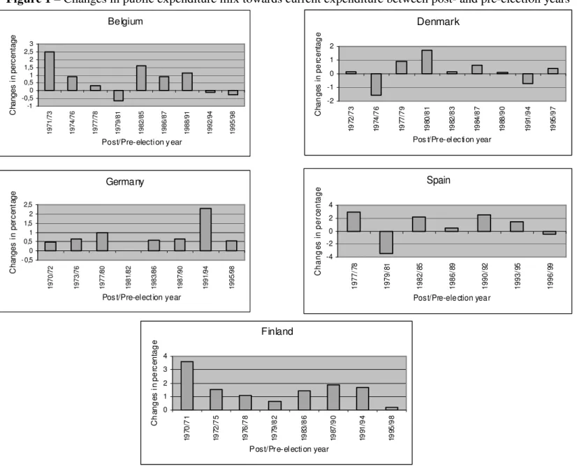
In Figure 1, Belgium, Denmark, Germany, Spain, and Finland support our analysis that manipulation on public expenditure composition between the post election year and the pre election year favours current expenditure increase. This occurs regardless of the degree of democratic maturity between EU countries and their economic dimension.
However, the SGP has a forceful role in moving public expenditure composition manipulation away from current expenditure, observed in decreases from 86% of the pre-election periods in the 70s to 69% in the 80s and 66% in the 90s. The breadth of public expenditure manipulation also decreased from a 1.9 percentage points current expenditure average in the 70s to a 1.1 percentage points expenditure average in the following two decades.
[
insert figure 1 about here]
Through data on the 15 EU member states, the research focus is based on public expenditure cycles and its relation to election terms. Empirical findings show that firstly elections continue to play an important part in the shaping of public expenditure cycles in the EU. Central governments increase their share of current expenditure whenever elections draw near. Secondly, when we look at the subset of countries where coalition governments dominate, budgetary bias in favour of current expenditure is reinforced.
The paper is organised as follows. Section 2 presents the theoretical background and raises some questions on the issue. Section 3 describes the variables employed and respective data sources. Section 4 reports on procedures used in the estimation process and section 5 presents the results of the empirical application. Section 6 concludes the paper.
Theoretical background
Theory predicts that political budget cycles become less prevalent as information becomes more symmetric, as voter awareness increases and as democracy evolves. In well established democracies, as in the EU, with high standards of government transparency, budget manipulation around election times should not be expected at aggregate levels, as voters sense such manipulations are opportunistic and tend to penalise governments in upcoming elections. Public choice theory claims that politicians maintain own selfish interests that are not completely contingent on re-election concerns. If politicians perceive that budget manipulation of certain expenditure categories will render other political dividends and if re-election chances are not too heavily affected, politicians are still motivated to manipulate budget items for selfish gain.
Barreira and Baleiras (2005) propose a theoretical model that shows that manipulation on expenditure categories is to be expected even when voters hold complete information on the extent of budget manipulation, in this way compromising public expenditure mix. The driving force behind this type of behaviour from politicians is twofold:
(i) politicians are uncertain of reappointment and as such prefer certain ego-returns to an expected rewards from office from prospective employers in the event of nonreelection;1
(ii) expenditure categories do not necessarily produce political dividends in simultaneous time frames: current expenditure typically produces quick political returns while politicians are still in office, however, capital expenditure requires some time to generate political dividends. This time lag on utility achieved from capital expenditure causes politicians to spend more on current expenditure in pre-election periods even if this is not in tune to voter preferences in terms of public expenditure composition.
The framework consists of a budgetary cycle of two periods, denoted i, i = 1,2 whereby the incumbent must decide the budgetary shares of consumption (gA) and capital expenditure (gB) for each period, with gA+gB =1, for simplicity. An incumbent decides on the expenditure composition at the beginning of each period and his/her utility from public expenditure is v gi for i= ,A B, which means he/she has no prior bias for any type of outlay. This satisfaction can only be acquired while the incumbent is in office. Additionally, v( )⋅ is twice continuously differentiable, with
' 0, '' 0
v > v < . Any decision an incumbent makes on consumption expenditure will
1 Only in office politicians can extract a certain level of utility. Any political dividends that can only be attained after elections enter probabilistically into politicians’ utility.
yield immediate political dividend payoff, i.e. during the same period the expenditure is incurred. However, any euro spent on capital expenditure during period 2 will only give the incumbent utility in the following period if re-elected, an outcome that is uncertain. This delay phenomenon also occurs in period 1. However, as capital expenditure decisions reached in period 1 become perceptible in period 2, the incumbent’s utility from that expenditure is certain. Moreover, there is an election after period 2 and the incumbent knows that there are job opportunities besides government positions, in case of electoral defeat. In such case he/she has the possibility to be employed by business community and earn an income y. The satisfaction from the outside payoff is x y( ), with x' 0> , which is obtained if the incumbent loses the election.
Voters decide their ballot based on an assessment of the incumbent’s performance. Such assessment is captured by s, where
s a w g= 1A +w gA2 + −1 a w g1B +w gB2 ,
with w' 0, '> w' 0< , and parameter a (a∈0 1, ) represents the voters’ preferences for budget composition between consumption and capital expenditure. When a>0 5. < . , a bias for consumption (capital) expenditure is observed. Re-election a 05 probability, π, is thus a function of voters’ satisfaction level: π π= s , π∈
[ [
0,1 and π'> 0. If we assume that voters prefer no cycle (a=0.5) during the two-period tenure, then, as the difference between gA and gB increases for each period, s becomes smaller reducing the chances for the incumbent’s re-election. Business community, as part of the electorate, shares voters’ preferences. Hence, the politician’s outside income is endogenously formed as y y s= ( ), with y′>0.The incumbent’s inter-temporal utility function can be observed as: U v g= 1A +v g1B +v g2A +πv gB2 + −1 π x y .
Formally, the fiscal choice of period 1 generates an ego return v gA1 in period 1
and an ego return v g1B in period 2; the fiscal choice of period 2 induces ego return
v g2A in period 2 and an expected ego return πv g
B2 in period 3, if re-elected.
Moreover, period 3 expected utility, in case of electoral defeat, is given by 1−π x y .
From this framework emerges a prediction that can be empirically tested. Proposition 1. The inter-temporal political expenditure cycle.
Even when the electorate shows no preference for a cycle a = 05. ,
i) a political budget cycle is found in the pre-election period, given by gA2 > . , and 0 5
In interpreting this result we can say that by taking into consideration the chance of losing the upcoming contest and since capital expenditure in period 2 flows probabilistically forward into the next period utility, the incumbent is led to discount the future utility from being in office according to re-election prospects. Under this framework, the incumbent has thus an incentive to spend on consumption expenditure rather than on capital expenditure.
The choices of the EU framework for the empirical application relies on assumptions the theoretical model considers regarding information voters possess. With the degree of information voters receive, consequent of a consolidating democratic regime, surfaces the adequacy of empirically testing the theoretical prediction on a set of stabilised democracies, such as those within the EU. According to Islam (2003), findings show that EU countries2 comprise the set of countries that better represent information transparency. Islam provides a “transparency” index that measures the frequency with which economic data are published in countries around the world.3 The spread of such information assumes greater accuracy in developed societies since it is commonly accepted that the electorate absorbs an extensive array of information through the news media.4 Information access allows voters to better measure the performance of politicians with relatively low cost.
We propose an empirical application to validate the hypothesis formulated in the theoretical background. We look to identify manipulation in the budget mix, opportunistically-induced by central governments, i.e., the budget weight associated to current and capital expenditure near election periods, which lead to a political budget cycle. In the next section, we present the dependent and independent variables used for estimation purposes.
2 OECD countries for example include countries with significantly differentiated democracies, considering European consolidated democracies and relatively recent democracies like Slovak Republic, Poland or Hungary. As such, a much more heterogeneous degree of political information, accessible to voters, is expected on OECD countries.
3 Nine of the fifteen EU countries represent the highest rank in the transparency indicator, analogous to countries like the United States, Canada and Australia. Countries with high-income levels are argued to carry levels of “transparency” that are twofold, with the exception of some oil producing countries.
4 The WorldAudit Organisation conducted a survey on 186 countries which rated each country’s press freedom, studying both political and economic pressures on the media (Electronically available at: http://www.worldaudit.org). The score goes from 0 to 100, with higher scores indicating less freedom. Countries scoring 0 to 30 are regarded as having “free” media, 31 to 60, “partly free” and 61 to 100, “not free”. When the EU comprised 15 countries, 7 countries scored below 15, 7 countries presented scores between 15 and 30 and only one achieved a score above 30.
Variables and data
The current section describes the variables to be included in the empirical model specification: the dependent variable denominated EXP and 8 independent variables. 5 The sample covers 10 EU countries6 for a period of 32 years. The countries considered in our analysis include: Belgium, Denmark, Finland, France, Germany, Greece, Italy, Luxembourg, Portugal and Spain. Published data are available on a year-to-year basis from 1970 to 2001.
The dependent variable
The dependent variable is specified as being the difference between current and capital expenditure weights (EXP), which takes the value zero when the two weights are equal.7 Thus, the variable captures the bias of certain expenditure types, i.e., a positive value represents a bias towards current expenditure and a negative value indicates a bias towards capital expenditure. We impose fiscal conservatism ensuring that, in each year, an amount of public expenditure is normalised to one. We focus merely on the public expenditure mix effect discarding the overall public expenditure size effect.
The independent variables
In the empirical application we specify a model that includes electoral variables, given that our primary goal is to evaluate how elections determine government manipulation of the public expenditure mix, as well as other control variables to capture institutional and economic differences across countries. More precisely, the empirical model specified for estimation considers eight explanatory variables. Two dummies relating to legislative election dates (ELEC0 and ELEC1), the unemployment rate (UER), the consumer price index (CPI), government’s ideological position (IDEOL),
5 See Appendix 1 for a detailed description of the variables used on the empirical model specification.
6 The sample covers the 15 countries that comprised the EU. For statistical reasons explained subsequently we use only a subset of countries in the empirical application.
7 Defining the dependent variable in such a way allows us to examine the budget bias towards one of the two types of public expenditure. Since full budget is the sum of current and capital expenditure, we can state that defining only the weight of the current expenditure will have the same effect, since current expenditure weight increases as capital expenditure weight decreases. However, the model does not look to explain the evolution of public expenditure components but rather how the deviation between the two components develop.
government’s power in the assembly (LPS), voter turnout (VPR) and population weight over than 65 years of age (POP65).8
Our aim is to investigate the relationship between the electoral cycle and the budget composition bias towards current expenditure. In this sense, the first two explanatory variables included in the model specification are dummy variables corresponding to the two periods in which a government is in power: the pre-election and post-election periods. Following Schuknecht (2000)’s approach, we adopt as ELEC0 and ELEC1, respectively, as descriptors.9
We include two economic variables in order to capture possible economic cycles that might restrain governments from public expenditure manipulation such as the unemployment rate (UER) and the consumer price index (CPI). Three political variables are also considered: the government’s ideological position (IDEOL), the government’s power to decide alone on public expenditure composition (LPS) and the voter turnout rate (VPR).
In order to distinguish between opportunistic (office-seeking) and partisan motivations, we introduce a variable indicating ideologically induced bias on budget composition in our model specification, since parties that make up a government are not ideologically neutral.
An ideological variable assumes a relevant feature because it provides information on governmental preferences regarding public expenditure.10 Given the classification of parties into a scale, we consider an IDEOL variable as defined in Appendix 1. The lower the IDEOL value the higher the expected budget bias towards current expenditure.11
8 See Appendix 2 for a detailed variable data source list. The Appendix 3 presents the descriptive statistics by variable and country considered in the empirical model.
9 There are several approaches proposed in the literature for the definition of the electoral dummies. After analysing the alternative specifications, namely those proposed by Blais and Nadeau (1992), by Dalen and Swank (1996), by Franzese (2000a), by Carmignani (2000), by Chang (2001), by Shi and Svensson (2002), by Huber, Kocher and Sutter (2003) and by Mulas-Granados (2003), we considered the Schuknecht’s approach the most reasonable to capture the phenomena this work looks to develop.
10 It is commonly accepted that left-wing parties tend to spend more on current expenditure than right-wing parties. Cusack (1997) shows that in industrialised democracies, during 1955 to 1989, ideological preferences of ruling parties and levels of governt spending are related. Left-wing parties tend to favour redistribution, thus providing greater public expenditure while right-wing parties prefer the untrammelled workings of the market system, which reduces government spending. Dalen and Swank (1996) use Dutch data (1953-1993) to determine that left-wing cabinets attach greater importance to social security and health care while right-wing cabinets value expenditure on infrastructure and defence.
11 During the 70s, Greece, Portugal and Spain faced a dictatorial to a democratic transition. Under dictatorship, governments do not face reappointment concerns. With guaranteed reappointment, governments prefer to spend on current expenditure rather than on capital expenditure since the latter type of expenditure gives utility with a period delay. The incentive of dictatorial regimes to manipulate budget composition is greater when compared to democratic regimes. Accordingly, we consider the value for this variable to be zero during the period in which democracy is absent in Greece, Portugal and Spain.
The next political variable measures the parliamentary power of governments. We observe different realities across EU parliaments. Some EU countries have a much fractionated parliament, with many parties having a reduced share of total parliamentary seats. As would be expected, government coalitions are the likely outcome in such countries. Coalition governments are dominant in countries like Belgium, Denmark, Italy, Luxembourg, Netherlands and Finland, for example. In contrast, however, Portugal, Spain, Greece and United Kingdom maintain a tradition of single party governments.
In order to capture departures resulting from the relative differences from governments to induce a budget composition bias, we introduce the variable LPS that measures the weight of the larger party in a parliamentary assembly.12 We show later, through the empirical application, that single party governments do not perform equally to coalition governments, often revealing differences in terms of public expenditure manipulation across EU countries.13
Governments are aware that by excessively manipulating public expenditure, reelection may be at stake. In the proposed model, we present an innovative feature that contemplates voters as do not being induced in error by fiscal illusion. As such, the voter turnout rate (VPR) might be a constraining force on a government’s freedom to manipulate public expenditure,14 a hypothesis that we look to empirically validate.
If we believe that voters have no preference bias regarding public expenditure composition, we can still expect an increase on current expenditure in pre-election years. Firstly because governments are uncertain about re-appointment and secondly because capital expenditure generates an ego-return with a one-period delay. Given these circumstances, governments know that the higher the turnout rate,15 the greater the electoral fall will be when public expenditure deviates from that desired by voters. Greater voter turnout expressing dissatisfied to government expenditure suggests the
12 The importance of government’s polarisation to the electorally-induced manipulation of public expenditure is well documented and derives from two facts. Firstly, is expected to feel less responsible for budget options taken since the probability of reelection is substantially smaller compared to a one party government. As the re-election chances lessen, the party in power is dissuaded from upkeep concerns, increasing budget bias during office. Secondly, attrition is greater where a leading party of considerable size in a ruling coalition does not exist, thus leading to more systematic public expenditure manipulations.
13 Several studies on the coalition government effects on budget performance like Roubini and Sachs (1989), de Haan, Sturm and Beekhuis (1999), Volkering and de Haan (2001) and Huber, Kocher and Sutter (2003) show that governments in coalition with multi-party composition tend to overspend, inducing an increase on budget deficit.
14 Hicks and Swank (1992) support this argument establishing a positive relation between turnout and welfare efforts of governments in western democracies. Also, Mueller and Stratmann (2003) report a positive link between electoral participation and the degree of distributive policies.
15 Belgium turnout rate is a particular case since more than 90% of voter participation has occurred during the last three decades, made compulsory by law.
need for a more responsible and loyal government to their constituents, less intent on budget manipulation.
Finally, we include a social variable, POP65, which corresponds to the weight of the population over 65. This variable looks to capture budget composition bias towards current expenditure induced through social transfers and health care expenditure.
Methodology
Panel data unit root tests
Testing for unit roots in time series is common practice among empirical studies.16 However, testing for unit roots in panels is a recent process, with major developments in nonstationary panel models originating in mid-1990s. Recent attention has been given to panel data issues arising from numerous time series procedures applicated to panels, such as nonstationarity, spurious regressions17 and cointegration.
Levin and Lin (1992, 1993)18, Im, Pesaran and Shin (2003) and Maddala and Wu (1999), are authoritative references of panel unit root tests that rely on cross sectional independence.
To deal with the presence of cross-sectional dependency, Chang (2002) proposed a panel unit root test based on non-linear instrumental variable (IV) estimation of the usual Augmented Dickey-Fuller (ADF) type regression for each cross-sectional unit, using as instruments non-linear transformations of the lagged levels. The test statistic is defined as an average of individual IV t-ratios, which is asymptotically normal, and does not require the tabulation of critical values.
In this paper, we apply the Im, Pesaran and Shin test, henceforth IPS, and the Chang panel data unit root tests. The panel unit root tests that we employ are joint
16 See Stock (1994), Maddala and Kim (1998), and Phillips and Xiao (1998) for a overview of unit root tests in time series.
17 Considering two random vectors
it
Y and Xitthat are I
( )
1 , or equivalently, nonstationary, and without cointegration between them, then if a time series regression for a certain i is performed, the regression coefficient will have a nondegenerative limit distribution and the regression is characterised as spurious. The problem is only extenuated when the panel has large cross sectional and time series dimensions.18 The Levin and Lin test treats panel data as being composed by homogeneous cross-sections, thus performing a test on a pooled data series. The homogeneity hypothesis can be considered too restrictive since panel data can be composed by several cross-sections with different autoregressive coefficients. The main argument is that under the alternative hypothesis the same convergence rate across countries can bias the panel data unit root tests. Imposing homogeneity when coefficient heterogeneity is present in cross-sectional data can lead to misleading conclusions. The IPS panel data unit root test presents an alternative to overcome this restriction.
hypothesis tests in the sense that all units of a panel contain a unit root. When the joint null hypothesis is rejected it is possible that one or a few time series in the panel contribute to this finding. Cumulatively, given that these tests allow the autoregressive parameter to differ across cross sections under the alternative, then the rejection of the null hypothesis means that not all units of the panel contain a unit root. Effectively, a mixture of stationary and nonstationary time series can cohabit in the same panel data. Given the limitations associated with the previous panel unit root tests, we use an alternative test that allows for the presence of contemporaneous cross-correlation and heterogeneous serial correlation of the regression residuals as suggested by Breuer, McNown and Wallace (2002), hereafter BNW.
The main advantage of BNW test is that it allow us to determine which cross sectional series reject the null hypothesis of a unit root and which do not. The BNW test uses a SUR framework for testing each panel unit under the null and the alternative hypothesis, exploiting the information in the error covariances to produce efficient estimators and potentially more powerful test statistics. The structure of hypothesis follows the ADF specification used in the IPS test procedure.
The panel specification that is used in the SURADF estimation is described as
' 1, 1 1, 1 1, 1, 1, 1 1, 1 ' , , 1 , , , , 1 ... . . i i p t t j t j t t j p N t N N t N j N t j N t N N t j y y y z y y y z ρ ϕ γ ε ρ ϕ γ ε − − = − − = ∆ = + ∆ + + ∆ = + ∆ + +
The null hypothesis is H0:ρi =0 for each time series of the panel.
In general the SURADF is a more powerful test than the ADF test. For the I 0 time series, BNW show, based on median rejection rates, that SURADF has twice the power or even more then a single equation ADF to reject the null hypothesis when the autoregressive coefficient on each I 0 time series is 0.90. However, these power gains vanish for an autoregressive coefficient between 0.95 and 0.99.
The BNW test has however a disadvantage that emerges from the fact that the test statistics obtained through SURADF model have no standard distributions, implying the need for simulation of the necessary critical values. To compute these critical values it is necessary to consider the estimated covariance matrix for the system under analysis, the sample size and the number of panel units. This means that each study has its own critical values.
Our main panel data unit root test results are presented in Appendix 4.19 As indicated, the rejection of the null of a panel unit root by IPS or Chang’s tests does not imply that all time series are stationary. Moreover, when we look at the BNW test the
19 The detailed panel unit root tests are not reported here but are available from the author upon
rule appears to be a mix between stationary and non-stationary time series when the presence of cross sectional dependence is taken in to account.
The panel unit root tests presented and the mixed characteristics of the panels considered in the empirical application serve as the underlying argument for our next analysis.
When some of the individual time series that compose a panel show evidence of the existence of unit roots, then an estimation procedure like mean group estimation or pooled mean group estimation, described in the following sub-section, seems to be appropriate. This argument is reinforced when we suspect of heterogeneous autoregressive coefficients on the dependent variable across cross-sections. The mean group estimation or pooled mean group estimation can be used despite of the stationarity or nonstationarity characteristics of the regressors, thus constituting an important advantage.
Further, under heterogeneous slopes and under small sample properties of panel time series estimators, Coakley, Fuertes and Smith (2001) show that by allowing for I 1 errors, which results in spurious time series regressions, the pooled and mean group estimators appear unbiased.
Estimation procedure
For our empirical application we use panel data of T and N, time dimension and cross-section dimension, respectively. A country panel of the type we employ in this paper raises some important econometric methodological issues that are not always fully appreciated. There is increasing use of panel data samples in macroeconomics, based on development in the micro areas in which panels have traditionally been used. Dynamic models are, however, common in typical time series rather than static models. When the cross-section dimension is added and the lagged dependent variable is introduced, some important problems may surface as a result of heterogeneity in the model parameters. Some earlier studies employing panel data techniques did not allow for the possibility of panel heterogeneity beyond fixed effects. However, neglecting slope heterogeneity causes the disturbances to be serially correlated as well as contemporaneously correlated with the included regressor(s). Pesaran and Smith (1995) observe that the larger the degree of parameter heterogeneity, the greater the bias of these models.
Traditional studies on electoral budget cycles using panel data techniques have relied on the fixed effects model. However, new branches of study have questioned the adequacy of this model which only allows heterogeneity across countries through the intercept, arguing that slope homogeneity seems unlikely when countries are at
different stages in their economic development and have diverse institutions, customs and social norms. In order to accommodate these problems, we apply the pooled mean group estimation method (PMG), recently proposed by Pesaran, Shin and Smith (1999), to estimate dynamic specifications that impose homogeneity restrictions on long-run coefficients if and only when such restrictions are not statistically rejected.
The PMG estimation procedure is an intermediate estimator between the total slope heterogeneity as is assumed by the Mean Group estimator (MG) proposed by Pesaran and Smith (1995) and the heterogeneity that is considered in the dynamic fixed-effects estimator (DFE). In fact, the PMG estimator proposed by Pesaran et al. (1999) is more reliable than the previous two estimators discussed since it involves both pooling and averaging. The PMG estimator allows the intercepts, short-run coefficients and error variances to differ across countries, but imposes equality of one or more of the long-run coefficients. The main argument is that while it is implausible for the dynamic specification to be common to all countries, it is at least conceivable that the long-run parameters of the model may be common. In this sense, the PMG estimator imposes some homogeneity across countries compared with the MG estimator, which bears quite strong assumptions, like the independence of parameters and regressors, as well as strictly exogenous regressors. The PMG estimator allows for heterogeneity on the short-run effects absent in the DFE estimator which tends to underestimate the short-run effects and overestimate the average long-run effects under the presence of parameter heterogeneity.20 In this case, none of the usual remedies such as the instrumental variables estimation technique or variable differencing addresses the problem.
Cumulatively, the PMG estimator reveals to be quite robust to outliers 21 as well as to the choice of lag order specified in the model; moreso than the MG estimator, whose estimates can be highly influenced by such factors. The PMG estimator is a two-step procedure: the first is the joint estimation of the homogeneous long-run coefficients across countries through the Maximum Likelihood procedure and the second is the estimation of the error-correction coefficients and the short-run parameters of the model, on a country-by-country basis. The PMG estimation has been applied in several areas of research, for instance in panel data studies on
20 This statement is true regardless of the stationary or integrated nature of the variables. In fact,
Pesaran, Smith and Im (1996) argue that with integrated variables under slope heterogeneity a differentiating cointegrating relation across countries is found. Thus, incorrectly imposing common slope parameter for all countries introduces an I
( )
1 component in the disturbances, leading to inconsistent parameter estimators, even in the static form.21 In small samples, the MG estimator, being an unweighted average, is excessively sensitive to the inclusion of outlying country estimates. The PMG estimator performs better in this regard because it produces estimates that are similar to weighted-averages of the respective country-specific estimates, where the weights are given according to their precision (i.e., the inverse of their corresponding variance-covariance matrix).
economic growth (see for example, Bassanini and Scarpetta (2001), Bassanini, Scarpetta and Hemmings (2001), Asteriou and Price (2005), Gupta, Clements, Baldacci and Mulas-Granados (2005)); on labour markets changes (see Serres, Scarpeta and Maisonneuve (2002) and Fedderke, Shin and Vaze (2003)); on private saving rates growth (see Serres and Pelgrin (2002)); and on public budget balance growth (see Hallerberg and Strauch (2002)).
To simplify the exposition and using an Autoregressive Distributed Lag Model− ARDL(p,q,q,...,q) 22, the first step to PMG estimation is defined by the following equation: yit ij i t jy x j p ij i t j j q i it = − + + + = = − λ , δ' , µ ε 1 0 , (1)
with i= 1 2, ,...,N and t= 1 2, ,...,T and where yit is the dependent variable, xit
represents the set of explanatory variables and µi indicates the country fixed-effects.
We implement the second step through the following error correction model (ECM): ∆yit i i ty i i tx ij∆yi t j ∆x j p ij i t j j q i it = − + − + − + + + = − − = − φ , 1 β' , 1 λ* , δ*' , µ ε 1 1 0 1 , (2) where φi λij j p = − − = 1 1 , βi δij j q = =0 , λij λim m j p * = − = +1 , with j=1 2, ,...,p−1, and δij δim m j q * = − = +1 , with j =1 2, ,...,q−1.
In expression (2), φi is the error correction coefficient measuring the speed of
adjustment towards the long-run equilibrium.
The lag order used into ARDL specification is obtained from each country’s unrestricted regression model, where the selection is done according to the best Schwarz Bayesian Criterion (SBC) associated with each lag specification. The homogeneous lag order used in the ARDL model is determined by the highest most common lag specification that is chosen in the individual regressions.
The consistency and efficiency of the PMG estimates depend on several conditions regarding the specification. In order to assess the robustness of the empirical model some previous diagnostic statistics are applied on individual country ARDL equation. The usual battery of statistical tests include the Breusch−Godfrey (1978) test for residual serial correlation, the Ramsey (1969) RESET test for functional form misspecification, the Jarque-Bera (1980) test for errors normality, and the White (1980) test for homoscedasticity. The former two statistics and the latter one have a
22 The advantage of the use of ARDL models is presented in Pesaran and Shin’s (1999) article. The authors point out that these models are robust to integration and cointegration properties of the regressors, and for sufficiently high lag orders they are immune to the endogeneity problem, at least as far as the long-run properties of the model are concerned.
chi-square distribution with p-degrees of freedom, where p represents the number of lags included in regressions, and the third statistic have a chi-square distribution with two degrees of freedom.
Returning to expression (1), the set of explanatory variables is restricted to an autoregressive process, which does not depend on contemporaneous values of y. This restriction arises from the assumption that there is only one long-run relationship betweenxandy. However, as Calderón, Loayza and Servén (2000) point out, there is a possibility for x to be endogenous in the sense that the factors that affect x may be correlated with contemporaneous effects in y. As such, we thus consider the correction proposed by Calderón et al. (2000) for the PMG estimation, which is necessary under the existence of contemporaneous correlation across variables. The simultaneous causation possibility, i.e., the existence of a feedback between y and x, is captured in what follows by a non-zero σεu. Using the single equation framework,
Calderón et al. derive the parameterisation that should be introduced to account for the endogeneity of x.
We now use, for the sake of simplicity, an ARDL 11, model derived from expression (1): yt =λyt−1+δ10xt+δ11xt−1+ +a εt, for each country, where
xt =ρxt−1+ut, and εt t u ~iid 0,Σ , Σ = σ σ σ σεεε ε u u uu . The contemporaneous correlation between εt and ut is represented by a linear regression of εt on ut as,
ε σ σε η t u uu t t u
= + , where ηt is distributed independently from ut(and, thus, from xt).
In this way, the new residual in the ARDL 11, model is uncorrelated with all explanatory variables and given as
yt yt u x x a uu t u uu t t =λ − + δ +σ + − − + + σε δ ρ σσε η 1 10 11 1 .
The ECM implied by the ARDL 11, given above can be expressed, analogously, as in expression (2)
(
)
10 11 1 1 10 1 1 1 u uu t t t u t t uu a y y x x ε ε σ δ δ ρ σ φ λ λ σ δ η σ − − + + − ∆ = − − − − + + ∆ + .Therefore, the long-run relationship can be represented as
(
)
10 11 * * * 1 1 1 u uu a y x ε σ δ δ ρ σ λ λ η + + − = + − − + .Regression specification and implementation
Our empirical model initially includes fifteen EU member countries in the analysis. However, after performing the four robustness tests on cross-section regressions, we observe that only ten countries satisfy the necessary conditions to be included in the PMG estimation. In particular, at a conventional statistical level, we observe evidence of serial correlation in the residuals of one country, a functional form misspecification in another country and the evidence of non-normality of residuals in four countries (see Appendix 5). Effectively, then, we exclude from our analysis those countries that do not fulfil the necessary conditions to be included in the regression estimation. Thus, the model specification is estimated comprehending the following ten countries: Belgium, Denmark, Germany, Greece, Spain, France, Italy, Luxembourg, Portugal and Finland.
In addition, as required for a long-run relationship to exist, the estimated convergence coefficient φi is negative in the ten countries and statistically significant
in 8 of them.
Our empirical application estimates the parameters of the following model specification: , 1 10, 20, 30, 41, , 1 50, 51, , 1 60, 70, 80, exp exp 0 1 + 65 it i i i t i it i it i it i i t i it i i t i it i it i it it
elec elec uer cpi ideol ideol lps vpr pop
µ λ δ δ δ δ δ δ δ δ δ ε − − − = + + + + + + + + + + +
Conditional on the long-run homogeneity hypothesis, we can rewrite the above model as: , 1 0 1 2 3 51, 4 , 1 5 , 1 6 7 8 exp 0 1 exp + 65 i t it it it it i i it it i t i t it it it
elec elec uer
ideol
cpi ideol lps vpr pop
θ θ θ θ φ δ ε θ θ θ θ θ − − − − − − − − ∆ = − ∆ + − − − − where φi = −1 λi , θ δ δ λ z z z i = + − 0 1 1 , with z= 1 2, ,...,8 and θ µ λ 0 =1−i i .
The PMG estimator assumes long-run homogeneity, meaning that θ θi = , for
i= 1 2, ,...,N , where θi = −β φi i.
We test the long-run homogeneity assumption and we find that the homogeneity of PMG long-run coefficients estimate is not rejected by the modified version of the Hausman (1978) test, proposed by Pesaran, Shin and Smith (1999). 23 The Hausman statistic test for the long-run coefficients is defined as
hθ = θMG−θPMG V θMG −V θPMG θMG−θPMG −
^ ^ ' ^ ^ ^ ^ 1 ^ ^
.
Under the slope homogeneity hypothesis, the Hausman statistic is asymptotically distributed as χ2 with θ degrees of freedom.
23 Hausman test for each long-run coefficient and for the joint long-run coefficients are available from the author upon request.
Results
In accordance with our expectations regarding the electoral cycle and its effect on the government manipulation of the public expenditure composition, we anticipate the parameter associated with ELEC0 as being significantly positive and ELEC1 as either positive or negative with no statistical significance. A positively estimated parameter of ELEC0 variable indicate that pre-election periods induce governments to influence budget composition towards current expenditure. An estimated parameter of ELEC1 variable not statistically significant suggests that there is no empirical evidence of government bias in terms of budget composition in post-election periods.
In observing column A in Table 1, we can verify that governments do manipulate budget composition towards current expenditure in the pre-election years, as the PMG estimate for ELEC0 parameter demonstrates. Also, the long-run coefficient24 for the post-election period, referred to as ELEC1, is not statistically significant, suggesting that there is no evidence that governments change the composition of public expenditure during these periods. In other words, we find evidence of a political budget cycle opportunistically-induced in the pre-election years though we do not observe any tendency for a cycle in the post-election periods.25
[
insert table 1 about here]
We expect a positive parameter estimate for unemployment, that is, higher unemployment causes an increase of current expenditure through welfare transfers, and a negative parameter estimate for the consumer price index, especially in variable estimations subject to time lags, following theoretical arguments that indicate budgets to play a stabilisation role which controls inflation through a contraction on current expenditure. Given the rivalry in consumption of welfare expenditure as directly related to the number of older citizens in the population, we anticipate a positive sign for the POP65 parameter estimated.
We observe that the economic variable parameters estimated are statistically significant in determining public expenditure composition. More precisely, we observe that the UER and POP65 regressors positively influence a budget bias
24 The short-run effects are not reported here by space convenience but are available from the author upon request. Furthermore, the main objective of this study is to test for the existence of political budget cycles, which does not require a detailed analysis of results regarding short-run effects.
25 We perform a sensitivity analysis to the parameter estimates in order to assess the robustness of results to variation of country coverage by eliminating one country at a time and re-running the PMG estimation procedure. Taking into account the width of confidence intervals (coef 1.96stdD
−
+ ), the ELEC0 and ELEC1 parameter estimates reveal to be stable.
towards current expenditure (a natural outcome) and the CPI regressor, with a year delay, refrain governments in increasing this type of public expenditure to avoid inflation.
We anticipate a negative sign to the estimated parameter of the IDEOL political variable. Since public expenditure manipulation occurs irrespective of partisan influences, we expect that the ideological position of a government does not significantly determine manipulation on the budget composition.
If the major parliamentary party retains a significant fraction of parliamentary seats, the party is less likely to manipulate budget composition in pelection years, as re-election is expected. However, if the largest parliamentary party shares only a small proportion of seats the reverse is likely to occur. Such parties are potentially more ego-rent dependent in terms of budget bias towards current expenditure (party holds fewer electorates). As such, we anticipate a negative sign for the estimated political variable (LPS) parameter.
In terms of political variables, the results are not so optimistic as they do not appear be relevant in explaining public expenditure composition. However, caution must be drawn from these findings given relatively small sample analysis. After performing a sensitivity test on the parameters estimated, we confirm that the parameter estimates for the political variables are very sensitive to the subset of countries included in the analysis, thereby suggesting that we cannot definitely ensure whether these variables actually affect public expenditure composition.
We expect that the greater the number of voters bailouts, the smaller the incentive for governments to engage in excessive current expenditure manipulation. This result is, however, only expected if voters preferences are prone to capital expenditure or if voters have no preference regarding the public expenditure mix. On the other hand, if voters prefer current expenditure, we can expect increased budget bias towards current expenditure given supported pre-election practices. Ultimately, since voters preferences are not observable, the turnout variable effect on the public expenditure mix remains an empirical issue. If the estimated parameter of the VPR variable takes a negative sign this would suggest that voters have a disciplinary force on governments who manipulate current expenditure. An estimated parameter with a positive sign would represent that voters have a preferential bias towards current expenditure. 26
The relationship between the number of effective voters in an election (VPR variable) and the composition of public expenditure reveals to be ambiguous. Although being statistically significant in our case, we observe that the long-run coefficient is also sensitive to the countries covered by the estimation. The long-run
26 Franzese (2000b) argues that in OECD countries higher voter turnout produces more transfers since there is a greater electoral representation of the lower classes.
estimates of VPR are unstable since their sign and significance level can vary substantially, allowing either a significant negative value or a significant positive value, depending on the countries covered by the analysis. Given these results, we were unable to assess the impact turnout may hold on public expenditure composition and consequently specific constituency preferences in terms the budget mix and governmental practices. In order to overcome the limitations of our small sample size, a different public expenditure partition should perhaps be considered, namely, between targeted and non-targeted expenditures, directions for a future work.
We reconsider whether observing an entire set of observations for all countries did not come at a cost. Namely, including dictatorial regimes during part of a seventy-year study span may have contributed towards estimated parameter bias, thus rendering ambiguous results for some variables. To evaluate whether the mix of governmental regimes influenced our findings we re-ran the PMG procedure that started with a 1978 data series, when all ten countries were following democratic regimes. We report the main results in column B of Table 1.
We observe that when dictatorial regimes are excluded from the analysis, the political budget cycle in pre-election years become more statistically significant. The economic and social variables remain statistically relevant. Within the political variables LPS emerges as being statistically significant, showing evidence of sensitivity in the countries analysed. This result can be influenced by the structure of the government power considered in the estimation procedure, since estimation included countries governed by single party governments and multi-party governments (coalition governments). We then determined that isolating the two effects would provide us with further results and as such reperformed the PMG procedure considering now only multi-party governments. The estimated parameters are presented in column C of Table 1.
For purposes of estimation we consider only seven countries, thus excluding Greece, Spain and Portugal. Interestingly, in comparing the results obtained under this subset of countries with our former findings, we determine that once correction for contemporaneous correlation is made, the PMG estimates of the electoral cycle are strengthened. In fact, there is evidence that countries with higher fractionated power resulting from coalition governments are more prone to have pre-election manipulation of public finances on current expenditure. This is to be predictably expected in multi-party governments that anticipate an upcoming election loss, in that they prefer to maximise their utility spending on current expenditure as much as possible in the pre-election periods. It also seems that countries with multi-party governments slightly increase their current expenditure in the post-election periods. This could be interpreted as a reaction by those parties holding a minority position in
government. Under these circumstances, parties want to satisfy some fringes of their electorate and increase specific types of public transfers in the post-election period.
Figure 1 provides us with the indication of public expenditure mix manipulation by coalition governments in five out of the seven countries considered. In fact, we report a systematic and significant bias induced on budget by the German and Finnish governments. This phenomenon corresponds to literature findings27 that state coalition governments submit to strong internal forces, leading to a more pronounced manipulation on public expenditure composition. Balassone and Giordano (2001) report a similar result on budget deficit, observing in eight EU countries a tendency for coalition governments to increase the budget deficit.
Accordingly, we can say that single party governments, given higher re-election chances, are less prone to manipulate public expenditure. Single party governments know that in the likely event of re-election, governments will retrieve utility from decisions made in the pre-election periods regarding capital expenditure, although visible only in the next legislature. This expectation reduces government incentive to excessively increase current expenditure in the pre-election periods.
When we take those countries where coalition governments prevail, we observe that the ideology and the turnout variables are statistically significant. This follows from our earlier argument that when governments need to share power with other parties, turnout becomes a more relevant variable since each party looks to please their respective constituents, accomplishing target expenditures. Similarly, differences on ideology appear to be important. However, contrary to our expectations and to early work on the issue (see for example de Haan and Sturm (1997)) it seems that right-wing governments tend to spend more on current expenditure. In a more recent study, Darby, Li and Muscatelli (2004) present similar findings to ours, supporting the claim that right-wing governments spend less on capital expenditure, and that multi-party minorities do not favour public capital as a result of greater re-election uncertainty.
Further, our sub-sample study of seven countries corresponds to central governments of well-established democracies which, according to Brender and Drazen (2005), are typically less prone to change the overall size of the budget. A political budget cycle may continue to exist on public expenditure composition besides on an aggregate level. Identifying whether an established democracy and dominating coalition governments holds significant bearing on electoral budget cycle remains an unanswered question and opens possibilities for further research.
27 Hallerberg and Hagen (1999) show that EU states with multi-party governments are not willing to delegate to one actor the ability to monitor and penalise those hamper budget agreements. Hallenberg and Hagen state that a strong finance minister is only feasible in countries where one-party governments are the norm. Although ministers of coalition government can cooperate in a prisoner’s dilemma game, a budget game, whose solution is unlikely since it involves the need for monitoring and penalising all those involved who may have other priority arrangements.
Concluding remarks
The main purpose of the current paper is to empirically investigate continued politically-induced cycles on public expenditure composition. We achieve findings that support theoretical predictions.
We applied a pooled mean group estimation method to a system of dynamic equations to analyse the effects of electoral, economic and political variables on public expenditure composition. This econometric technique allows for the speed of convergence as well as for short-term dynamics and variances to be different across countries, unlike most panel data approaches that impose homogeneity restrictions on all of these parameters.
In contrast to some common findings, claiming that a political budget cycle is more easily expected in developing countries where the asymmetry information phenomenon is common, an empirical test on EU countries shows that such a manipulation still occurs in developed countries, where voters have large access to information.
In looking at the impact of election terms on public finances in terms of government public expenditure manipulation, we find evidence of an electorally-induced increase of current expenditure. Besides the electoral cycle, the dynamic analysis reveals that economic variables influence public expenditure. The expenditure component that is directly related to the unemployment rate and to the number of older people in the population suggests an increase on current expenditure since these variables influence public transfers. The inflation rate with one-period delay induces reduced current expenditure, suggesting that budget composition also plays a stabilising role. Other variables such as government ideology or turnout are not conclusive in terms of their effects on public expenditure composition. The weight of the largest party in the parliament reveals to be a relevant variable only for countries where single party governments prevail.
Further, multi-party governments are more sensitive to public expenditure manipulation, causing a bias on budget composition in post-election periods as well. Under reduced party re-election chances in multi-party governments, each party will attempt to please its electorate with counter ego-return benefits from ministers outside office after upcoming elections, as suggested in Barreira and Baleiras (2005).
References
Akhmedov, A. & Zhuravskaya E. (2004). Opportunistic political cycles: Test in a Young Democratic Setting. Working Paper No47, School of Social Science, Institute for Advanced Study.
Asteriou, D. & Price, S. (2005). Uncertainty, investment and economic growth: evidence from a dynamic panel. Review of Development Economics 9(February): 277-288.
Balassone, F. & Giordano, R. (2001). Budget deficits and coalition governments. Public Choice 106(3-4): 327-349.
Barreira, A.P. & Baleiras, R.N. (2005). Elections and the public expenditure mix. Mimeo.
Bassanini, A. & Scarpetta, S. (2001). Does human capital matter for growth in OECD countries? Evidence from pooled mean-group estimates. OECD Economics Department Working Paper 282(January): 1-28.
Bassanini, A., Scarpetta, S. & Hemmings, P. (2001). Economic growth: The role of policies and institutions. Panel data evidence from OECD countries. OECD Economics Department Working Paper 283(January): 1-68.
Beck, T., Clarke, G., Groff, A., Keefer, P. & Walsh, P. (2001). New tools and new tests in Comparative Political Economy: The Database of Political Institutions. World Bank Economic Review 15(1): 165-176.
Blais, A. & Nadeau, R. (1992). The electoral budget cycle. Public Choice 74(4): 389-403.
Brender, A. & Drazen, A. (2005). Political budget cycles in new versus established democracies. Journal of Monetary Economics 52(7): 1271-1295.
Breuer, J.B., McNown, R. & Wallace, M. (2002). Series-specific unit root tests with panel data. Oxford Bulletin of Economics & Statistics 64(5): 527-546.
Breusch, T.S. (1978). Testing for autocorrelation in dynamic linear models. Australian Economic Papers 17(31): 334-355.
Buti, M. & Noord, P. (2003). Discretionary fiscal policy and elections: The experience of the early years of EMU. OECD Economics Department Working Paper 351(March): 1-16.
Calderón, C., Loayza, N. & Servén, L. (2000). External sustainability: A stock equilibrium perspective. World Bank Policy Research Working Paper 2281(January): 1-48.
Carmignani, F. (1999). Measures of political instability in multiparty governments: A new data set with econometric applications. Working Paper 9916, Department of Economics, Glasgow University.
(2000). Political bias in fiscal policy formation: an econometric analysis of coalition systems. Working Paper 28, Dipartimento di Economia Politica, Università degli Studi di Milano-Bicocca.
Castles, F.G. & Mair, P. (1984). Left-right political scales: Some “experts” judgements. European Journal of Political Research 12(March): 73-88.
Chang, E.C.C. (2001). Electoral budget cycles under alternative electoral systems. Paper presented at the annual meeting of the American Political Science Association, San Francisco, September.
Chang, Y. (2002). Nonlinear IV unit root tests in panels with cross-sectional dependency. Journal of Econometrics 110(2): 261-292.
Coakley, J., Fuertes A.-M. & Smith, R. (2001). Small sample properties of panel time-series estimators with I(1) errors. Birkbeck College Discussion Paper 3(July): 1-32. Cusack, T.R. (1997). Partisan politics and public finance: Changes in public spending
in the industrialized democracies: 1955-1989. Public Choice 91(3-4): 375-395. Dalen, H.P.V. & Swank, O.H. (1996). Government spending cycles: Ideological or
opportunistic? Public Choice 89(1-2): 183-200.
Darby, J., Li, C.-W. & Muscatelli, V.A. (2004). Political uncertainty, public expenditure and growth. European Journal of Political Economy 20(1): 153-179. de Haan, J. & Sturm, J.-E. (1997). Political and economic determinants of OECD
budget deficits and government expenditures: a reinvestigation. European Journal of Political Economy 13(4): 739-750.
de Haan, J., Sturm, J.-E. & Beekhuis, G. (1999). The weak government thesis: Some new evidence. Public Choice 101(3): 163-176.
Drazen, A. & Eslava, M. (2004). Political Budget Cycles without deficits? Paper presented at the annual meeting of the Public Choice Society, Baltimore-Maryland, March.
Eslava, M. (2005). Political budget cycles or voters as fiscal conservatives? Evidence from Colombia. Documento CEDE 2005-12(February): 1-38.
Fedderke, J., Shin, Y. & Vaze, P. (2003). Trade, technology and wage inequality: A dynamic panel data approach to the South African Manufacturing Sectors. Working Paper 106, Management School & Economics, University of Edinburgh.
Franzese, R.J. (2000a). Electoral and partisan manipulation of public debt in developed democracies, 1956-90. In R. Strauch & J. Von Hagen (eds.), Institutions, Politics and Fiscal Policy. Kluwer Academic Press, pp. 61-83.
(2000b). Political participation, income distribution, and public transfers in developed democracies. Paper presented at the American Political Science Association (APSA) Meeting, Boston, September.
Godfrey, L.G. (1978). Testing Against General Autoregressive and Moving Average Error Models when the Regressors Include Lagged Dependent Variables. Econometrica 46(6): 1293-1302.
Gupta, S., Clements, B., Baldacci, E. & Mulas-Granados, C. (2005). Fiscal policy, expenditure composition, and growth in low-income countries. Journal of International Money and Finance 24(3): 441-463.
Hallerberg, M. & Hagen, J. (1999). Electoral institutions, cabinet negotiations, and budget deficits within the European Union. In J.M. Poterba & J. Hagen (eds.), Fiscal Institutions and Fiscal Performance. Chicago: The University of Chicago Press: 209-232.
Hallerberg, M. & Strauch, R. (2002). On the cyclicality of public finances in Europe. Empirica 29(September): 183-207.
Hausman, J.A. (1978). Specification tests in econometrics. Econometrica 46(6): 1251-1271.
Hicks, A.M. & Swank, D.H. (1992). Politics, institutions, and welfare spending in industrialized democracies, 1960-82. American Political Science Review 86(3): 658-674.
Huber, G., Kocher, M. & Sutter, M. (2003). Government strength, power dispersion in governments and deficits in OECD-countries. A voting power approach. Public Choice 116(3-4):333-350.
Huber, J.D. & Inglehart, R.L. (1995). Expert interpretations of party space and party locations in 42 societies. Party Politics 1(1): 73-111.
Im, K.S., Pesaran, M.H. & Shin, Y. (2003). Testing for unit roots in heterogeneous panels. Journal of Econometrics 115(1): 53-74.
Islam, R. (2003). Do more transparent governments govern better? World Bank Policy Research Working Paper 3077(June): 1-41.
Jarque, C.M. & Bera, A.K. (1980). Efficient tests for normality homocedasticity and serial independence of regression residuals. Economics Letters 6(3): 255-259. Laver, M. & Hunt, W.B. (1992). Policy and party competition. New York: Routledge,
Chapman and Hall.
Levin, A. & Lin, C.-F. (1992). Unit root tests in panel data: Asymptotic and finite-sample properties. Discussion Paper 92-23, Department of Economics, University of California - San Diego.
(1993). Unit root tests in panel data: New results. Discussion Paper 93-56, Department of Economics, University of California - San Diego.
Maddala, G.S. & Kim, I.-M. (1998). Unit roots, cointegration and structural change. Cambridge University Press.