Multi-attribute response of maize genotypes tested in different coastal regions of Brazil
Lúcio Borges de Araújo1*, Mario Varela Nualles2, Mirian Fernandes Carvalho Araújo1, Carlos Tadeu dos Santos Dias3
(1) Universidade Federal de Uberlândia. Av. João Naves de Ávila, 2.121 - Santa Mônica
CEP: 38400-902 - Uberlândia - MG - Brasil
(2) Departamento de Matemática. Instituto Nacional de Ciencias Agrícolas. Carretera
Tapaste, km 3 ½. San José de las Lajas. Apdo Postal, 3700. Habana. Cuba.
(3) Escola Superior de Agricultura Luiz de Queiroz. Av. Pádua Dias, 11. Piracicaba. São
Paulo- Brasil.
(*) Corresponding author<[email protected]>
ABSTRACT: This work applies the Three Mode Principal Components Analysis to: analyze simultaneously the multiple attributes; to fit of models with additive main effects and multiplicative interaction effects (AMMI models) and the regressions models on sites (SREG models); to evaluate respectively the multivariate response of the genotype × environment interaction and the mean response of 36 genotypes of corn tested in 4 locations in Brazil. The results were presented by joints plots to identify the best genotypes for their adaptability and performance in the set of attributes.
Key words: Biplots, Genotype × Environment interaction, three-way data, Principal Components Analysis.
INTRODUCTION
The multi-environment trials are conducted to estimate the genetic stability, to evaluate the performance of the genotypes in different environmental conditions and to quantify and interpret the genotype × environment interaction (GEI), in such a way to select the best genotypes that will be recombined and planted in other years and other environments in the next selection cycle. Some statistical models are used to evaluate the behavior of the genotypes; the most recently proposed methods are based on the singular value decomposition of the GEI matrix.
of these models was made by [2], which applies the PCA to decompose the two way interaction in several multiplicative terms. This model was called as additive main effects and multiplicative interaction effects model (AMMI) by Gauch [3].
Another class of the Linear-bilinear model used in multi-environment trials is the Sites Regression Model (SREG) described by [4]. In this case the main objective is to evaluate the response of the genotype in each environment. The basic difference in relation to AMMI models is that the effect of genotype is introduced into the residual interaction. This model was used by [5] for clustering of environmental data with no cross-interaction.
Gabriel, [6] describes the least squares adjustment of the AMMI model, first estimating the additive effects of the model and then making the decomposition in singular values of the matrix (Z) of interaction residuals. The results can be interpreted by graphics called biplot [7] that reflects in reduced dimensions the most important aspects of the GEI, in the case the AMMI model, or the performance of genotypes in different environments, for the case of the model SREG.
The researchers in the multi-environmental trials evaluate multiple attributesand must select the best, genotypes taking in to account its adaptability and performance in the set of attributes. With the AMMI and SREG models it is possible to study the genotypes in a single attribute. However, if we want a response with multiple attributes it is necessary to apply a statistical technique that allows working with three-dimensional structure data.
In [8] a Three Mode Principal Components Analysis (PCA3) is proposed, in order to find the least squares estimates in the model of Tucker [9]. This procedure was used to study the GEI with multiples attributes ([10]; [11], [12], [13]). The method also was applied by [14] and [15] to study the three-way interaction in agricultural experiments where genotypes are tested in different locations over several years.
In this work we used the Three Mode Principal Component Analysis to explain, in reduced dimensions, the most important aspects of multi-attribute performance of the 36 genotypes of maize tested in 4 regions of Brazil. First, we studied the GEI using the AMMI model with multiple attributes as described ([15], [16]) and finally studied the genotypes in relation to the mean environment for multiple attributes as described in [17].
Data are from experiments with 36 genotypes of maize (first mode, i = 1,…,36), evaluated in 4 locations of Brazil (S1: Rio BrancoAC, S2: MilagresCE, S3: Linhares -ES, cohesive soil Oxisol, S4: Linhares--ES, soil-LVA-Distrophic LVD11) (second mode, j = 1,...,4). In each of the experiments 10 attributes were evaluated: X1: flowering (days), X2: plant height (cm), X3: corn-cob length (cm), X4: percentage of plants laid, X5: percentage of plants broken, X6 : final stand, X7: number of spikes, X8: percentage of patients corn-cobs, X9: weight of spikes (kg /ha), X10: weight of grains (kg /ha) (third mode, k = 1,...,10 ).
The data were obtained using a simple lattice design in duplicate 6 × 6 with 4 replications. Each plot consisted of two rows of 5m, used entirely. The spacing between rows was 1m and between hills it was 0.40m. Each plot consisted of 26 hills and each hole with 3 seeds. The seeds used in the tests were sent by the National Center for Research in Maize and Sorghum - CNPMS of Empresa Brasileira de Pesquisa Agropecuária - EMBRAPA, already counted, contained in envelopes coded with the number of genotype and number of the parcel.
Statistical Processing
Each attribute k (k=1,...,10) was calculated according to model the estimates corresponding to interactions: (yijk. - yi.k.- y.jk.+ y..k.) for AMMI model or (yijk.- y.jk.) for
SREG model, where yijk., represents the mean corresponding to attribute k for the
genotype i in location j; yi.k., represents the mean corresponding to the attribute k for the
genotype i; y.jk., represents the mean corresponding to the attribute k in location j and
y..k., represents the overall mean of the data for the attribute k. Two tridimensional
arrays (Z) were constructed with the values obtained using the AMMI model or the
SREG model, that is, for each model, the value zijk in the array Z represents the residue
to the genotype j in the location j, for the attribute k. Each array was applied to Three Mode Principal Components Analysis. Therefore, this methodology can be used for any data set.
Three Mode Principal Component Analysis
pqr kr jq P
p Q q
R r
ip
ijk a b c g
z
∑∑∑
= = =
=
1 1 1 .
where aip, bjq and ckr are the elements of the principal components matrix (A, B and C)
associated with each respective mode, and in this example, A is the principal
components matrix for the genotype mode, B is the principal component matrix for the
location mode and C is the principal component matrix for the attribute. G is a core
array of the three way, where the element gpqr represent the relationship between the pth
component of the first mode with the qth component of the second mode and with the
rth component of the third mode. P is the rank of the matrix Z1;2⊂3 that contains the
residuals of the interaction with all the variables, calculated as an AMMI model or as a SREG model. In this matrix the rows represent the levels of the genotypes and the columns represent combinations of the levels of locations and attributes. Similarly, Q and R are defined as the rank of matrices Z2;1⊂3 andZ3;1⊂2.
To select the number of principal components retained for each mode the algorithm proposed by [18] was used, based on successive eliminations until finding the optimal solution.
Biplot Representation for three markers matrices
A biplot is a simultaneous representation of rows and columns of a matrix (two- way array) in terms of directions and projections [7]. When we have several matrices, or when we are working with data contained in a three-way array, it’s necessary to project on the principal components of one of the modes. Suppose we are going to project onto the components of the second mode (locations) and Q1 represents the number of
principal components retained in this mode; then we have to obtain the matrices
A×Gq×B', q = 1 ,..., Q1 and require one biplot for each matrix. Gq is the part of G
associated with the component q of the second mode. This procedure is described by [8] and commonly called a joint plot.
RESULTS AND DISCUSIONS AMMI multi-attribute
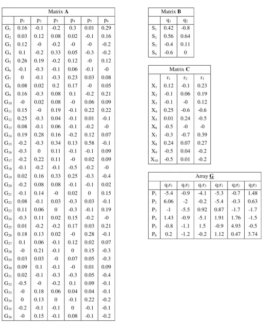
interaction obtained for the AMMI model with 10 attributes simultaneously. This solution explained 44.92% of the total variability, therefore this percentage is significant in relation to ten attributes measured in the research. The components associated with the genotype mode explain respectively 12.85%, 11.70%, 6.37%, 6.22%, 4.93% and 2.84%, the components of the location mode explaining respectively 25.49% and 19, 44% and the components of the attribute mode explaining respectively 22.6%, 11.6% and 11.0% of the total variability.
Table 1. 6 × 2 × 3 solution for AMMI model with Multiples Attributes.
Matrix A Matrix B
p1 p2 p3 p4 p5 p6 q1 q2
G1 0.16 -0.1 -0.2 0.3 0.01 0.29 S1 0.42 -0.8
G2 0.03 0.12 0.08 0.02 -0.1 0.16 S2 0.56 0.64
G3 0.12 -0 -0.2 -0 -0 -0.2 S3 -0.4 0.11
G4 0.1 -0.2 0.33 0.05 -0.3 -0.2 S4 -0.6 0
G5 0.26 0.19 -0.2 0.12 -0 0.12
G6 -0.1 -0.3 -0.1 0.06 -0.1 -0 Matrix C
G7 0 -0.1 -0.3 0.23 0.03 0.08 r1 r2 r3
G8 0.08 0.02 0.2 0.17 -0 0.05 X1 0.12 -0.1 0.23
G9 0.16 -0.3 0.08 0.1 -0.2 0.21 X2 -0.1 0.06 0.19
G10 -0 0.02 0.08 -0 0.06 0.09 X3 -0.1 -0 0.12
G11 0.15 -0 0.19 -0.1 0.22 0.22 X4 0.25 -0.6 -0.6
G12 0.25 -0.3 0.04 -0.1 0.01 -0.1 X5 0.01 0.24 -0.5
G13 0.08 -0.1 0.06 -0.1 -0.2 -0 X6 -0.5 -0 -0
G14 0.19 0.28 0.16 -0.2 0.12 0.07 X7 -0.3 -0.7 0.39
G15 -0.2 -0.3 0.34 0.13 0.58 -0.1 X8 0.24 0.07 0.27
G16 -0.3 0 0.11 -0.1 -0.1 0.09 X9 -0.5 0.04 -0.2
G17 -0.2 0.22 0.11 -0 0.02 0.09 X10 -0.5 0.01 -0.2
G18 -0.1 -0.2 -0.1 -0.5 -0.2 -0
G19 0.02 0.16 0.33 0.25 -0.3 -0.4 Array G
G20 -0.2 0.08 0.08 -0.1 -0.1 0.02 q1r1 q1r2 q1r3 q2r1 q2r2 q2r3
G21 -0.1 0.14 -0 0.02 0 0.15 P1 -5.4 -0.9 -4.1 -5.3 -0.7 1.48
G22 0.08 -0.1 0.03 -0.3 0.03 -0.1 P2 6.06 -2 -0.2 -5.4 -0.3 0.63
G23 0.11 0.06 0 -0.3 -0.1 0.19 P3 -1 -5.5 0.92 0.87 -1.7 -1.7
G24 -0.3 0.11 0.02 0.15 -0.2 -0 P4 1.43 -0.9 -5.1 1.91 1.76 -1.5
G25 0.01 -0.2 -0.2 0.17 0.03 0.21 P5 -0.8 -1.1 1.5 -0.9 4.93 -0.5
G26 0.18 0.13 0.02 -0 0.28 -0.1 P6 0.2 -1.2 -0.2 1.12 0.47 3.74
G27 0.1 0.06 -0.1 0.12 0.02 0.07
G28 -0 0.21 -0.1 0 0.15 -0.3
G29 0.03 0.03 -0 0.07 0.05 -0.3
G30 0.09 0.1 -0.1 -0 0.01 0.09
G31 0.02 -0.1 -0.3 -0.3 0.05 -0.4
G32 -0.5 -0 -0.2 0.1 0.09 -0.1
G33 -0 0.18 0.06 0.04 0.04 -0.1
G34 0 0.13 0 -0.1 0.22 -0.2
G35 -0.2 -0.1 -0.1 0 -0.1 -0.1
G36 -0 0.15 -0.1 0.08 -0.1 -0.2
Component 1 of the local mode is characterized by all the sites with relatively high weights (Matrix B, Table 1). This component is described by contrast between
sites S1 and S2 (Rio Branco-AC and Milages-CE) versus sites S3 and S4 (Linhares-ES
oxisol cohesive soil and Linhares-ES LVA-dystrophic- LVD11 soil).
Figure 1 shows the most important genotypes × locations interactions for the different attributes evaluated, mainly for the attribute X4 (percentage of plants laid). Genotype 19 interacts positively in locations S1 and S2 and negatively in locations S3 and S4 for attribute X4. Genotypes 18 and 31 have a behavior completely contrary to genotype 19, that is, they interact positively in the locations S3 and S4 and interact negatively in locations S1 and S2 for the attribute X4. In regard to variable X2 (plant height) the behavior of these genotypes is totally contrary to variable X4, e.g., the genotype 19 interacts negatively in locations S1 and S2 and positively in the locations S3 and S4 for the attribute X2.
Figure 1. Joint plot conditioned on the first component the location mode for AMMI model. Figure 1 also shows the contrast between the genotypes 9 and 12 of the genotypes 17, 24 and 32. The first group interacts positively in the attributes X6, X9 and X10 for locations S1 and S2 and negatively in these attributes for the locations S3 and S4. Genotypes 17, 24 and 32 have positive interaction in the attributes X1 and X8
-2 -1.5 -1 -0.5 0 0.5 1 1.5 2
-1.5 -1 -0.5 0 0.5 1 1.5 1 2 3 4 5 6 7 8 9 10 11 12 13 14 15 16 17 18 19 20 21 22 23 24 25 26 27 28 29 30 31 32 33 34 35 36 X1 X2 X3 X4 X5 X6 X7 X8 X9 X10
Axe 1 (12.29 %)
in the locations S1 and S2 but have negative interactions in locations S3 and S4 in these attributes.
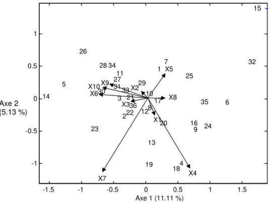
Figure 2 shows the projection biplot onto the second component of locations, which is dominated by contrast of the sites S1 and S2 with respective weights (-0.75 and 0.64) (Matrix B, Table 1). In this graphic it is possible to study the genotypes ×
locations interaction in different attributes for the locations S1 and S2. For example genotype 15 interacts positively in the local S1 for attribute X7 and interacts negatively in local S2 for this attribute. There is also the contrast of genotypes 4 and 18 in relation to genotype 26. The genotype 26 interacts positively with the attribute X4 in local S1 and interacts negatively in local S2 for this attribute, then in S2 there are a few percentage of plant laid and in S1 many percentage of plant laid. The contrast between the genotypes 5 and 14 in relation to the genotypes 6 and 35 for attributes X6, X9 and X10 can be observed. The first group had positive interactions with S2 and negative with S1, and showed that in the S2 there are high values of final stand, weight of spikes and weights of grains.
Figure 2. Joint plot conditioned on the second component the location mode for AMMI model
SREG multi-attribute
-1.5 -1 -0.5 0 0.5 1 1.5
-1 -0.5 0 0.5 1
1
2 3
4 5
6 7
8
9 10
11
12
13 14
15
16 17
18 19
20 21
22
23 24
25 26
27 28
29 30 31
32
33 34
35 36
X1 X2
X3
X4 X5
X6
X7
X8 X9
X10
Axe 1 (11.11 %)
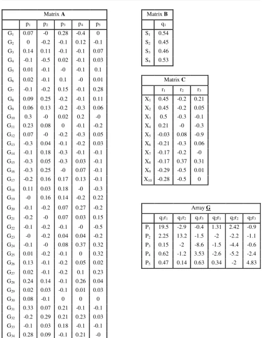
Table 2 shows the results of the 5 × 2 × 3 solution obtained by applying the Three Mode Principal Components Analysis to the three-way array containing the residuals of interaction for the SREG model with 10 attributes simultaneously. This solution explained 53.70% of the total variability. The components associated with the genotype mode explain respectively 27.69%, 13.34%, 6.96%, 3.77% and 1.94%, the components of the local mode explain 46.23% and 7.48% and the components of the mode attribute explain 27.96%, 17.31% and 8.42%. In this analysis the first component of the local mode is characterized by all the sites with relatively high weights (Matrix B,
Table 2).
Table 2. 5 × 2 × 3 solution for SREG model with multiples attributes.
Matrix A Matrix B
p1 p2 p3 p4 p5 q1
G1 0.07 -0 0.28 -0.4 0 S1 0.54
G2 0 -0.2 -0.1 0.12 -0.1 S2 0.45
G3 0.14 0.11 -0.1 -0.1 0.07 S3 0.46
G4 -0.1 -0.5 0.02 -0.1 0.03 S4 0.53
G5 0.01 -0.1 -0 -0.1 0.1
G6 0.02 -0.1 0.1 -0 0.01 Matrix C
G7 -0.1 -0.2 0.15 -0.1 0.28 r1 r2 r3
G8 0.09 0.25 -0.2 -0.1 0.11 X1 0.45 -0.2 0.21
G9 0.06 0.13 -0.2 -0.3 0.06 X2 0.45 -0.2 0.05
G10 0.3 -0 0.02 0.2 -0 X3 0.5 -0.3 -0.1
G11 0.23 0.08 0 -0.1 -0.2 X4 0.21 -0 -0.3
G12 0.07 -0 -0.2 -0.3 0.05 X5 -0.03 0.08 -0.9
G13 -0.3 0.04 -0.1 -0.2 0.03 X6 -0.21 -0.3 0.06
G14 -0.1 0.18 -0.3 -0.1 -0.1 X7 -0.17 -0.2 -0
G15 -0.3 0.05 -0.3 0.03 -0.1 X8 -0.17 0.37 0.31
G16 -0.3 0.25 -0 0.07 -0.1 X9 -0.29 -0.5 0.01
G17 -0.2 0.16 0.17 0.13 -0.1 X10 -0.28 -0.5 0
G18 0.11 0.03 0.18 -0 -0.3
G19 -0 0.16 0.14 -0.2 0.22
G20 -0.1 -0.2 0.07 0.27 -0.2 Array G
G21 -0.2 -0 0.07 0.03 0.15 q1r1 q1r2 q1r3 q2r1 q2r2 q2r3
G22 -0.1 -0.2 -0.1 -0 -0.5 P1 19.5 -2.9 -0.4 1.31 2.42 -0.9
G23 -0 -0.2 0.04 0.04 -0.2 P2 2.25 13.2 -1.5 -2 -2.2 -1.1
G24 -0.1 -0 0.08 0.37 0.32 P3 0.15 -2 -8.6 -1.5 -4.4 -0.6
G25 0.01 -0.2 -0.1 0 0.32 P4 0.62 -1.2 3.53 -2.6 -5.2 -2.4
G26 0.13 -0.1 -0.2 0.05 0.02 P5 0.47 0.14 0.63 0.34 -2 4.83
G27 0.02 -0.1 -0.2 0.1 0.23
G28 0.24 0.14 -0.1 0.26 0.04
G29 0.02 0.03 -0.1 0.01 0.03
G30 0.08 -0.1 0 0 0
G31 0.33 0.07 0.21 -0.1 -0.1
G32 -0.2 0.29 0.21 0.23 0.03
G33 -0.1 0.03 0.18 -0.1 -0.1
G35 0.11 0.08 0.15 0.16 0.05
G36 -0.1 0.15 0.34 -0.2 0
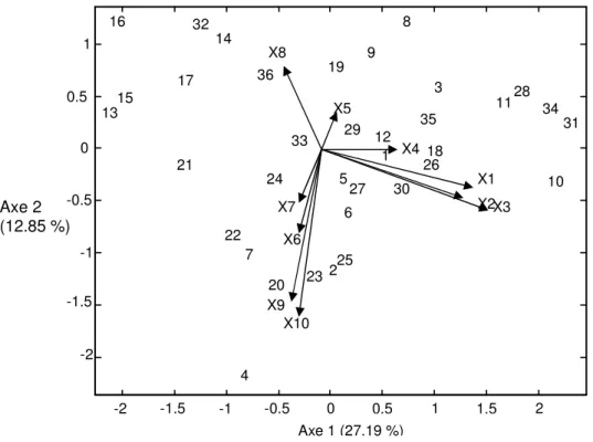
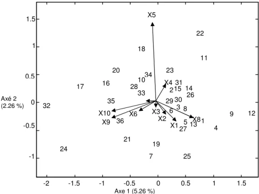
Figure 3 studies the behavior of the genotypes in relation to the mean environmental for different attributes. Genotypes 10, 11, 28, 31 and 34 are above mean environmental for the attributes X1, X2 and X3 in the 4 locations and, in contrast, the genotypes 13, 14, 15, 16, 17 and 32 has a performance below the mean environmental in these attributes. Genotype 4 has good performance in the variables X9 and X10 to the 4 sites in contrast to genotype 8 which is below the mean environmental in these attributes in the same locations. An opposite behavior occurs in the variable X8 in which genotype 4 is below mean environmental and genotypes 8, 14 and 32 have good performance.
Figure 3. Joint plot conditioned on the first component the location mode for SREG model
The second component of the local mode is characterized by local S2 and S4 with respective weights of -0.73 and 0.61 (Table 2, Matrix B). This component reflects
the contrast between these two locations. In the corresponding joint plot (Figure 4) it can be observed that genotypes 1, 4, 7, 9, 12 and 25 have good behavior with the
-2 -1.5 -1 -0.5 0 0.5 1 1.5 2
-2 -1.5 -1 -0.5 0 0.5 1 1 2 3 4 5 6 7 8 9 10 11 12 13 14 15 16 17 18 19 20 21 22 23 24 25 26 27 28 29 30 31 32 33 34 35 36 X1
X2 X3 X4 X5 X6 X7 X8 X9 X10
Axe 1 (27.19 %)
variable X8 for the local S4, but are below the mean environmental in local S2 for this same attribute. For the same genotypes the opposite happens, they have good performance in variable X5 for the local S2, but they are below mean environmental for the same attribute to the local S4.
Figure 4. Joint plot conditioned on the second component the location mode for SREG model. The fundamental difference between AMMI models with multiple attributes and SREG models with multiple attributes is that in the first case study the two-way interaction considering all the attributes while in the SREG model it is possible to study the multivariate behavior of genotypes in relation to the mean environmental.
CONCLUSIONS
Based on Three Mode Principal Components Analysis it is possible to work simultaneously with multiple attributes in the adjustment of AMMI and SREG models, so we can do a multivariate study of the most important aspects of the genotype × environment interaction and the response of genotypes in different environmental conditions.
-2 -1.5 -1 -0.5 0 0.5 1 1.5 -1
-0.5 0 0.5 1 1.5
1 2
3
4 5
6
7
8
9 10
11
12 13
14 15 16
17
18
19 20
21
22
23
24
25 26
27 28
2930 31
32
33 34
35
36
X1 X2 X3
X4 X5
X6
X8 X9
X10
Axe 1 (5.26 %) Axé 2
When we have many combinations of levels of factors the conditioned joint plot is a powerful tool to represent three arrays of markers, and gives us information on the most important aspects of the response of genotypes. It was possible to detect the combinations of genotypes × locations × attributes causing the significant interaction and the differential response, that is, identify the best genotypes in view of its adaptability and performance.
REFERENCES
[1] E.J. Williams, The interpretation of interactions in factorial experiments.
Biometrika,v.39, pp.65-81, 1952.
[2] H.F. Gollob, A statistical model which combines feature of factor analytic and analyses of variance techniques. Psykometrika, v.33, pp.73-115, 1968.
[3] H.G. Gauch, Model Selection and Validation for Yield Trials with Interaction.
Biometrics, v.44, pp.705-715, 1988.
[4] J. Crossa, P.L. Cornelius, Sites regression and shifted multiplicative model clustering of cultivar trials sites under heterogeneity of error variance. Crop Science,
v. 37, pp.405-415, 1997.
[5] J. Crossa, R.C. Yang, P.M. Cornelius, Studying crossover genotype × environment
interaction using linear-bilinear models and mixed models. Journal of Agricultural,
Biological and Environmental Statistics, v.9, pp.362-380, 2004.
[6] K.R. Gabriel, Least squares approximation of matrices by additive and multiplicative models. Journal of the Royal Statistical Society: Series B, v.40, pp.186–
196, 1978.
[7] K.R. Gabriel, The Biplot graphic display of matrices with applications to principal components analysis. Biometrika, v.58, pp.453-467, 1971.
[8] P.M. Kroonenberg, J. De Leeuw, Principal Component Analysis of Three-Mode Data by means of Alternating Least Squares Algorithms. Psychometrika, v.45,
pp.69-97, 1980.
[9] L.R. Tucker, Some mathematical notes on three-mode factor analysis.
[10] P.M. Kroonenberg, K.E. Basford, An investigation of multi-attribute genotype response across environments using three mode principal component analysis.
Euphytica, v.44, pp.109-123, 1989.
[11] K.E. Basford, P.M. Kroonenberg, I.H. Delacy, P.K. Lawrence, Multiattribute evaluation of regional cotton variety trials. Theoretical and Applied Genetics, v.79,
pp.225-324, 1990.
[12] J. Crossa, K.E. Basford, S. Taba, I.H. Delacy, E. Silva, Three mode analysis of maize using morphological and agronomic attributes measured in multilocation trials.
Crop Science,v.35, pp.1483-1491, 1995.
[13] M. Varela, V. Torres, Aplicación del análisis de Componentes Principales de Tres Modos en la caracterización multivariada de somaclones de King Grass. Revista
Cubana de Ciencia Agricola,v.39, pp.12-19, 2005.
[14] F.A. Van Eeuwijk, P.M. Kroonenberg, Multiplicative Models for Interaction in Three-Way ANOVA, with Applications to Plant Breeding. Biometrics, v.54,
pp.1315-1333, 1998.
[15] M.Varela, J. Crossa, R.J. Adish, K.J. Arun, R. Trethowan, Analysis of three way interaction including multi-attributes. Australian Journal of Agricultural Research,
v.57, pp.1185-1183, 2006.
[16] K.E. D´Andrea, M.E. Otegui, A.J. De La Vega, Multi-Attributte response of maize inbred managed environments. Euphytica, v.162,pp.381-384, 2008.
[17] M. Varela, J. Crossa, K.J. Arun, P.L. Cornelius, Y. Manes, Generalizing the Sites Regression Model to the three-way interaction including multiattributes. Crop Science,
v.49, pp.2043-2057, 2009.
[18] M.E. Timmerman, H.A.L. Kiers, Three-mode principal components analysis. Choosing the number of components and sensitivity to local optima. British Journal of