Volume 2011, Article ID 215843,6pages doi:10.1155/2011/215843
Research Article
Multiattribute Response of Maize Genotypes Tested in
Different Coastal Regions of Brazil
L ´ucio Borges de Ara ´ujo,
1Mario Varela Nualles,
2Mirian Fernandes Carvalho Ara ´ujo,
1and Carlos Tadeu dos Santos Dias
31Faculty of Mathematics, Federal University of Uberlˆandia, Avenida Jo˜ao Naves de ´Avila, 2.121, 38400-902 Uberlˆandia, MG, Brazil 2Department of Mathematics, Instituto Nacional de Ciencias Agr´ıcolas (INCA), km 3.5, San Jos´e de Las Lajas, 3700 Habana, Cuba 3Department of Exact Sciences, University of S˜ao Paulo, Avenida P´adua Dias, 11, 13418-900 Piracicaba, SP, Brazil
Correspondence should be addressed to L ´ucio Borges de Ara ´ujo,[email protected]
Received 21 March 2011; Revised 8 June 2011; Accepted 13 September 2011
Academic Editor: Ravindra N. Chibbar
Copyright © 2011 L ´ucio Borges de Ara ´ujo et al. This is an open access article distributed under the Creative Commons Attribution License, which permits unrestricted use, distribution, and reproduction in any medium, provided the original work is properly cited.
This work applies the three mode principal components analysis to analyze simultaneously the multiple attributes; to fit of models with additive main effects and multiplicative interaction effects (AMMI models) and the regressions models on sites (SREG models); to evaluate, respectively, the multivariate response of the genotype×environment interaction and the mean response of 36 genotypes of corn tested in 4 locations in Brazil. The results were presented by joint plots to identify the best genotypes for their adaptability and performance in the set of attributes.
1. Introduction
The multienvironment trials are conducted to estimate the genetic stability, to evaluate the performance of the genotypes in different environmental conditions, and to quantify and interpret the genotype × environment
interaction (GEI), in such a way to select the best geno-types that will be recombined and planted in other years and other environments in the next selection cycle. Some statistical models are used to evaluate the behavior of the genotypes; the most recently proposed methods are based on the singular value decomposition of the GEI matrix.
In [1], the two-way interaction using the principal components analysis (PCA) are explained and considered in their model only one multiplicative term. An extension of these models was made in [2], which applies the PCA to decompose the two-way interaction in several multiplicative terms. This model was called as additive main effects and multiplicative interaction effects model (AMMI) by Gauch [3].
Another class of the Linear-bilinear model used in multienvironment trials is the sites regression model (SREG) described by [4]. In this case, the main objective is to evaluate the response of the genotype in each environment. The basic difference in relation to AMMI models is that the effect of genotype is introduced into the residual interaction. This model was used in [5] for clustering of environmental data with no cross-interaction.
Gabriel [6] describes the least-square adjustment of the AMMI model, first estimating the additive effects of the model and then making the decomposition in singular values of the matrix (Z) of interaction residuals. The results can be interpreted by graphics called biplot [7] that reflects in reduced dimensions the most important aspects of the GEI, in the case the AMMI model, or the performance of genotypes in different environments, for the case of the model SREG.
attributes. With the AMMI and SREG models, it is possible to study the genotypes in a single attribute. However, if we want a response with multiple attributes, it is necessary to apply a statistical technique that allows working with three-dimensional structure data.
In [8], a three mode principal components analysis (PCA3) is proposed, in order to find the least-square estimates in the model of Tucker [9]. This procedure was used to study the GEI with multiples attributes [10–13]. The method also was applied by [14,15] to study the three-way interaction in agricultural experiments where genotypes are tested in different locations over several years.
In this work, we used the three mode principal compo-nent analysis to explain, in reduced dimensions, the most important aspects of multiattribute performance of the 36 genotypes of maize tested in 4 regions of Brazil. First, we studied the GEI using the AMMI model with multiple attributes as described in [15, 16] and finally studied the genotypes in relation to the mean environment for multiple attributes as described in [17].
2. Materials and Methods
Data are from experiments with 36 genotypes of maize (first mode,i =1,. . ., 36), evaluated in 4 locations of Brazil (S1:
Rio Branco-AC,S2: Milagres-CE, S3: Linhares-ES, cohesive
soil Oxisol, S4: Linhares-ES, soil-LVA-Distrophic LVD11;
second mode, j = 1,. . ., 4). In each of the experiments,
10 attributes were evaluated:X1: flowering (days),X2: plant
height (cm), X3: corn-cob length (cm), X4: percentage of
plants laid,X5: percentage of plants broken,X6: final stand, X7: number of spikes, X8: percentage of patients corn-cobs, X9: weight of spikes (kg/ha), and X10: weight of grains
(kg/ha) (third mode,k=1,. . ., 10).
The data were obtained using a simple lattice design in duplicate 6×6 with 4 replications. Each plot consisted of
two rows of 5 m, used entirely. The spacing between rows was 1 m and between hills it was 0.40 m. Each plot consisted of 26 hills and each hole with 3 seeds. The seeds used in the tests were sent by the National Center for Research in Maize and Sorghum—CNPMS of Empresa Brasileira de Pesquisa Agropecu´aria—EMBRAPA, already counted, and contained in envelopes coded with the number of genotype and number of the parcel.
2.1. Statistical Processing. Each attributek(k = 1,. . ., 10) was calculated according to model the estimates correspond-ing to interactions: (yi jk. − yi.k. − y. jk. + y..k.) for AMMI
model or (yi jk.−y. jk.) for SREG model, whereyi jk.represents
the mean corresponding to attribute k for the genotype i in location j; yi.k. represents the mean corresponding to the attribute k for the genotype i; y. jk. represents the mean corresponding to the attribute k in location j; y..k. represents the overall mean of the data for the attributek. Two tridimensional arrays (Z) were constructed with the values obtained using the AMMI model or the SREG model, that is, for each model, the valuezi jkin the arrayZrepresents the residue to the genotype j in the location j, for the
attributek. Each array was applied to three mode principal components analysis. Therefore, this methodology can be used for any dataset.
2.2. Three Mode Principal Component Analysis. The method consists of finding the least-square estimators for the Tucker model:
zi jk.=
P
p=1
Q
q=1
R
r=1
aipbjqckrgpqr, (1)
where aip, bjq, and ckr are the elements of the principal components matrix (A, B, and C) associated with each respective mode, and in this example, A is the principal components matrix for the genotype mode, Bis the prin-cipal component matrix for the location mode, and C is the principal component matrix for the attribute.Gis a core array of the three way, where the element gpqr represents the relationship between the pth component of the first mode with the qth component of the second mode and with therth component of the third mode.Pis the rank of the matrixZ1;2⊂3that contains the residuals of the interaction
with all the variables, calculated as an AMMI model or as an SREG model. In this matrix, the rows represent the levels of the genotypes and the columns represent combinations of the levels of locations and attributes. Similarly,QandRare defined as the rank of matricesZ2;1⊂3andZ3;1⊂2.
To select the number of principal components retained for each mode, the algorithm proposed by [18] was used, based on successive eliminations until finding the optimal solution.
2.3. Biplot Representation for Three Marker Matrices. A biplot is a simultaneous representation of rows and columns of a matrix (two-way array) in terms of directions and projections [7]. When we have several matrices, or when we are working with data contained in a three-way array, it is necessary to project on the principal components of one of the modes. Suppose we are going to project onto the components of the second mode (locations) and Q1
represents the number of principal components retained in this mode; then we have to obtain the matricesA×Gq × B′, q = 1,. . .,Q
1, and require one biplot for each matrix.
Gq is the part of G associated with the component q of the second mode. This procedure is described in [8] and commonly called a joint plot.
3. Results and Discusions
3.1. AMMI Multiattribute. Table1shows the results of the 6
× 2 × 3 solution obtained by applying the three mode
1
2
3 4
5
6 7 8
9 11 10
12
13
14
15
16 17
18 19
20 21
22 23
24
25 26
27
28 29
30
31
32 33
34 35
36
−2 −1.5 −1 −0.5 0 0.5 1 1.5 2 −1.5
−1 −0.5 0 0.5 1 1.5
Axe 1 (12.29%)
A
x
e
2
(7.14%)
X1
X2 X3
X4
X5
X6
X7 X8 X9
X10
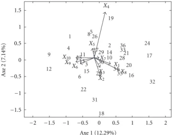
Figure 1: Joint plot conditioned on the first component the
location mode for AMMI model.
4.93%, and 2.84%, the components of the location mode explain, respectively, 25.49% and 19, 44%, and the com-ponents of the attribute mode explain, respectively, 22.6%, 11.6%, and 11.0% of the total variability.
Component 1 of the local mode is characterized by all the sites with relatively high weights (Matrix B, Table 1). This component is described by contrast between sites S1
andS2(Rio Branco-AC and Milages-CE) versus sitesS3and S4 (Linhares-ES oxisol cohesive soil and Linhares-ES
LVA-dystrophic-LVD11 soil).
Figure1shows the most important genotypes×locations
interactions for the different attributes evaluated, mainly for the attribute X4 (percentage of plants laid). Genotype 19
interacts positively in locationsS1andS2and negatively in
locations S3 andS4 for attributeX4. Genotypes 18 and 31
have a behavior completely contrary to genotype 19, that is, they interact positively in the locations S3 and S4 and
interact negatively in locationsS1andS2for the attributeX4.
In regard to variableX2(plant height), the behavior of these
genotypes is totally contrary to variable X4, for example,
the genotype 19 interacts negatively in locationsS1 andS2
and positively in the locationsS3andS4for the attributeX2.
Figure1also shows the contrast between the genotypes 9 and 12 of the genotypes 17, 24, and 32. The first group interacts positively in the attributes X6,X9, and X10
for locations S1 and S2 and negatively in these attributes
for the locations S3 and S4. Genotypes 17, 24, and 32
have positive interaction in the attributes X1 and X8 in
the locations S1 and S2 but have negative interactions in
locationsS3andS4in these attributes.
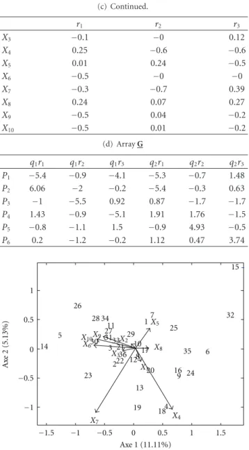
Figure 2 shows the projection biplot onto the second component of locations, which is dominated by contrast of the sites S1 andS2 with respective weights (−0.75 and
0.64) (Matrix B, Table 1). In this graphic, it is possible to study the genotypes×locations interaction in different
attributes for the locationsS1andS2. For example, genotype
15 interacts positively in the local S1 for attribute X7 and
interacts negatively in localS2for this attribute. There is also
Table 1: 6 × 2 × 3 solution for AMMI model with multiples
attributes.
(a) MatrixA
p1 p2 p3 p4 p5 p6
G1 0.16 −0.1 −0.2 0.3 0.01 0.29
G2 0.03 0.12 0.08 0.02 −0.1 0.16
G3 0.12 −0 −0.2 −0 −0 −0.2
G4 0.1 −0.2 0.33 0.05 −0.3 −0.2
G5 0.26 0.19 −0.2 0.12 −0 0.12
G6 −0.1 −0.3 −0.1 0.06 −0.1 −0
G7 0 −0.1 −0.3 0.23 0.03 0.08
G8 0.08 0.02 0.2 0.17 −0 0.05
G9 0.16 −0.3 0.08 0.1 −0.2 0.21
G10 −0 0.02 0.08 −0 0.06 0.09
G11 0.15 −0 0.19 −0.1 0.22 0.22
G12 0.25 −0.3 0.04 −0.1 0.01 −0.1
G13 0.08 −0.1 0.06 −0.1 −0.2 −0
G14 0.19 0.28 0.16 −0.2 0.12 0.07 G15 −0.2 −0.3 0.34 0.13 0.58 −0.1
G16 −0.3 0 0.11 −0.1 −0.1 0.09
G17 −0.2 0.22 0.11 −0 0.02 0.09
G18 −0.1 −0.2 −0.1 −0.5 −0.2 −0
G19 0.02 0.16 0.33 0.25 −0.3 −0.4
G20 −0.2 0.08 0.08 −0.1 −0.1 0.02
G21 −0.1 0.14 −0 0.02 0 0.15
G22 0.08 −0.1 0.03 −0.3 0.03 −0.1
G23 0.11 0.06 0 −0.3 −0.1 0.19
G24 −0.3 0.11 0.02 0.15 −0.2 −0
G25 0.01 −0.2 −0.2 0.17 0.03 0.21
G26 0.18 0.13 0.02 −0 0.28 −0.1
G27 0.1 0.06 −0.1 0.12 0.02 0.07
G28 −0 0.21 −0.1 0 0.15 −0.3
G29 0.03 0.03 −0 0.07 0.05 −0.3
G30 0.09 0.1 −0.1 −0 0.01 0.09
G31 0.02 −0.1 −0.3 −0.3 0.05 −0.4
G32 −0.5 −0 −0.2 0.1 0.09 −0.1
G33 −0 0.18 0.06 0.04 0.04 −0.1
G34 0 0.13 0 −0.1 0.22 −0.2
G35 −0.2 −0.1 −0.1 0 −0.1 −0.1
G36 −0 0.15 −0.1 0.08 −0.1 −0.2
(b) MatrixB
q1 q2
S1 0.42 −0.8
S2 0.56 0.64
S3 −0.4 0.11
S4 −0.6 0
(c) MatrixC
r1 r2 r3
X1 0.12 −0.1 0.23
(c) Continued.
r1 r2 r3
X3 −0.1 −0 0.12
X4 0.25 −0.6 −0.6
X5 0.01 0.24 −0.5
X6 −0.5 −0 −0
X7 −0.3 −0.7 0.39
X8 0.24 0.07 0.27
X9 −0.5 0.04 −0.2
X10 −0.5 0.01 −0.2
(d) ArrayG
q1r1 q1r2 q1r3 q2r1 q2r2 q2r3 P1 −5.4 −0.9 −4.1 −5.3 −0.7 1.48
P2 6.06 −2 −0.2 −5.4 −0.3 0.63
P3 −1 −5.5 0.92 0.87 −1.7 −1.7 P4 1.43 −0.9 −5.1 1.91 1.76 −1.5
P5 −0.8 −1.1 1.5 −0.9 4.93 −0.5
P6 0.2 −1.2 −0.2 1.12 0.47 3.74
1
2 3
4 5
6 7
8
9 10
11
12
13 14
15
16 17
18 19
20 21
22
23 24
25 26
27 28
29
30 31
32
33 34
35 36
−1.5 −1 −0.5 0 0.5 1 1.5 −1
−0.5 0 0.5 1
Axe 1 (11.11%)
A
x
e
2
(5.13%)
X1 X2
X3
X4 X5
X6
X7
X8
X9 X10
Figure 2: Joint plot conditioned on the second component the
location mode for AMMI model.
the contrast of genotypes 4 and 18 in relation to genotype 26. The genotype 26 interacts positively with the attributeX4in
localS1and interacts negatively in localS2for this attribute,
then in S2 there are a few percentage of plant laid, and
in S1 many percentage of plant laid. The contrast between
the genotypes 5 and 14 in relation to the genotypes 6 and 35 for attributesX6,X9, andX10 can be observed. The first
group had positive interactions withS2and negative withS1
and showed that in theS2there are high values of final stand,
weight of spikes, and weights of grains.
3.2. SREG Multiattribute. Table2shows the results of the 5×
2×3 solution obtained by applying the three mode principal
components analysis to the three-way array containing the residuals of interaction for the SREG model with 10 attributes simultaneously. This solution explained 53.70%
Table 2: 5 × 2 × 3 solution for SREG model with multiples
attributes.
(a) MatrixA
p1 p2 p3 p4 p5
G1 0.07 −0 0.28 −0.4 0
G2 0 −0.2 −0.1 0.12 −0.1
G3 0.14 0.11 −0.1 −0.1 0.07
G4 −0.1 −0.5 0.02 −0.1 0.03
G5 0.01 −0.1 −0 −0.1 0.1
G6 0.02 −0.1 0.1 −0 0.01
G7 −0.1 −0.2 0.15 −0.1 0.28
G8 0.09 0.25 −0.2 −0.1 0.11
G9 0.06 0.13 −0.2 −0.3 0.06
G10 0.3 −0 0.02 0.2 −0
G11 0.23 0.08 0 −0.1 −0.2
G12 0.07 −0 −0.2 −0.3 0.05
G13 −0.3 0.04 −0.1 −0.2 0.03
G14 −0.1 0.18 −0.3 −0.1 −0.1
G15 −0.3 0.05 −0.3 0.03 −0.1
G16 −0.3 0.25 −0 0.07 −0.1
G17 −0.2 0.16 0.17 0.13 −0.1
G18 0.11 0.03 0.18 −0 −0.3
G19 −0 0.16 0.14 −0.2 0.22
G20 −0.1 −0.2 0.07 0.27 −0.2
G21 −0.2 −0 0.07 0.03 0.15
G22 −0.1 −0.2 −0.1 −0 −0.5
G23 −0 −0.2 0.04 0.04 −0.2
G24 −0.1 −0 0.08 0.37 0.32
G25 0.01 −0.2 −0.1 0 0.32
G26 0.13 −0.1 −0.2 0.05 0.02
G27 0.02 −0.1 −0.2 0.1 0.23
G28 0.24 0.14 −0.1 0.26 0.04
G29 0.02 0.03 −0.1 0.01 0.03
G30 0.08 −0.1 0 0 0
G31 0.33 0.07 0.21 −0.1 −0.1
G32 −0.2 0.29 0.21 0.23 0.03
G33 −0.1 0.03 0.18 −0.1 −0.1
G34 0.28 0.09 −0.1 0.21 −0
G35 0.11 0.08 0.15 0.16 0.05
G36 −0.1 0.15 0.34 −0.2 0
(b) MatrixB
q1
S1 0.54
S2 0.45
S3 0.46
S4 0.53
(c) MatrixC
r1 r2 r3
X1 0.45 −0.2 0.21
(c) Continued.
r1 r2 r3
X3 0.5 −0.3 −0.1
X4 0.21 −0 −0.3
X5 −0.03 0.08 −0.9
X6 −0.21 −0.3 0.06
X7 −0.17 −0.2 −0
X8 −0.17 0.37 0.31
X9 −0.29 −0.5 0.01
X10 −0.28 −0.5 0
(d) ArrayG
q1r1 q1r2 q1r3 q2r1 q2r2 q2r3 P1 19.5 −2.9 −0.4 1.31 2.42 −0.9
P2 2.25 13.2 −1.5 −2 −2.2 −1.1
P3 0.15 −2 −8.6 −1.5 −4.4 −0.6 P4 0.62 −1.2 3.53 −2.6 −5.2 −2.4
P5 0.47 0.14 0.63 0.34 −2 4.83
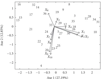
of the total variability. The components associated with the genotype mode explain, respectively, 27.69%, 13.34%, 6.96%, 3.77%, and 1.94%, the components of the local mode explain 46.23% and 7.48%, and the components of the mode attribute explain 27.96%, 17.31%, and 8.42%. In this analysis the first component of the local mode is characterized by all the sites with relatively high weights (MatrixB, Table2).
Figure3studies the behavior of the genotypes in relation to the mean environmental for different attributes. Geno-types 10, 11, 28, 31, and 34 are above mean environmental for the attributesX1,X2, andX3 in the 4 locations and, in
contrast, the genotypes 13, 14, 15, 16, 17, and 32 have a per-formance below the mean environmental in these attributes. Genotype 4 has good performance in the variablesX9 and X10 to the 4 sites in contrast to genotype 8 which is below
the mean environmental in these attributes in the same locations. An opposite behavior occurs in the variable X8
in which genotype 4 is below mean environmental and genotypes 8, 14, and 32 have good performance.
The second component of the local mode is characterized by localS2andS4with respective weights of−0.73 and 0.61
(Table 2, MatrixB). This component reflects the contrast between these two locations. In the corresponding joint plot (Figure4), it can be observed that genotypes 1, 4, 7, 9, 12, and 25 have good behavior with the variableX8for the local S4, but are below the mean environmental in local S2 for
this same attribute. For the same genotypes, the opposite happens, they have good performance in variable X5 for
the local S2, but they are below mean environmental for
the same attribute to the localS4.
The fundamental difference between AMMI models with multiple attributes and SREG models with multiple attributes is that in the first case study, the two-way interaction considering all the attributes, while in the SREG model, it is possible to study the multivariate behavior of genotypes in relation to the mean environmental.
1 2 3 4 5 6 7 8 9 10 11 12 13 14 15 16 17 18 19 20 21 22 23 24 25 26 27 28 29 30 31 32 33 34 35 36
−2 −1.5 −1 −0.5 0 0.5 1 1.5 2 −2
−1.5 −1 −0.5 0 0.5 1
Axe 1 (27.19%)
A x e 2 (12.85%) X1 X2X3 X4 X5 X6 X7 X8 X9 X10
Figure 3: Joint plot conditioned on the first component the
location mode for SREG model.
1 2 3 4 5 6 7 8 9 10 11 12 13 14 15 16 17 18 19 20 21 22 23 24 25 26 27 28 29 30 31 32 33 34 35 36
−2 −1.5 −1 −0.5 0 0.5 1 1.5 −1
−0.5 0 0.5 1 1.5
Axe 1 (5.26%)
A x e 2 (2.26%) X1 X2 X3 X4 X5 X6 X8 X9 X10
Figure 4: Joint plot conditioned on the second component the
location mode for SREG model.
4. Conclusions
Based on three mode principal components analysis, it is possible to work simultaneously with multiple attributes in the adjustment of AMMI and SREG models, so we can do a multivariate study of the most important aspects of the genotype×environment interaction and the response of
genotypes in different environmental conditions.
When we have many combinations of levels of factors, the conditioned joint plot is a powerful tool to represent three arrays of markers and gives us information on the most important aspects of the response of genotypes. It was possible to detect the combinations of genotypes ×
locations×attributes causing the significant interaction and
References
[1] E. J. Williams, “The interpretation of interactions in factorial experiments,”Biometrika, vol. 39, pp. 65–81, 1952.
[2] H. F. Gollob, “A statistical model which combines features of factor analytic and analysis of variance techniques,” Psychome-trika, vol. 33, no. 1, pp. 73–115, 1968.
[3] H. G. Gauch, “Model selection and validation for yield trials with interaction,”Biometrics, vol. 44, pp. 705–715, 1988. [4] J. Crossa and P. L. Cornelius, “Sites regression and shifted
multiplicative model clustering of cultivar trial sites under heterogeneity of error variances,”Crop Science, vol. 37, no. 2, pp. 405–415, 1997.
[5] J. Crossa, R. C. Yang, and P. L. Cornelius, “Studying crossover genotype x environment interaction using linear-bilinear models and mixed models,”Journal of Agricultural, Biological, and Environmental Statistics, vol. 9, no. 3, pp. 362–380, 2004. [6] K. R. Gabriel, “Least squares approximation of matrices by
additive and multiplicative models,” Journal of the Royal Statistical Society: Series B, vol. 40, no. 2, pp. 186–196, 1978. [7] K. R. Gabriel, “The biplot graphic display of matrices with
application to principal component analysis,”Biometrika, vol. 58, no. 3, pp. 453–467, 1971.
[8] P. M. Kroonenberg and J. De Leeuw, “Principal component analysis of three-mode data by means of alternating least squares algorithms,”Psychometrika, vol. 45, no. 1, pp. 69–97, 1980.
[9] L. R. Tucker, “Some mathematical notes on three-mode factor analysis,”Psychometrika, vol. 31, no. 3, pp. 279–311, 1966. [10] P. M. Kroonenberg and K. E. Basford, “An investigation of
multi-attribute genotype response across environments using three-mode principal component analysis,”Euphytica, vol. 44, no. 1-2, pp. 109–123, 1989.
[11] K. E. Basford, P. M. Kroonenberg, I. H. Delacy, and P. K. Lawrence, “Multiattribute evaluation of regional cotton variety trials,”Theoretical and Applied Genetics, vol. 79, no. 2, pp. 225–234, 1990.
[12] J. Crossa, K. Basford, S. Taba, I. Delacy, and E. Silva, “Three-mode analyses of maize using morphological and agronomic attributes measured in multilocational trials,” Crop Science, vol. 35, no. 5, pp. 1483–1491, 1995.
[13] M. Varela and V. Torres, “Aplicaci ´on del an´alisis de Com-ponentes Principales de Tres Modos en la caracterizaci ´on multivariada de somaclones de King Grass,”Revista Cubana de Ciencia Agricola, vol. 39, pp. 12–19, 2005.
[14] F. A. Van Eeuwijk and P. M. Kroonenberg, “Multiplicative models for interaction in three-way ANOVA, with applica-tions to plant breeding,”Biometrics, vol. 54, no. 4, pp. 1315– 1333, 1998.
[15] M. Varela, J. Crossa, R. J. Adish, K. J. Arun, and R. Trethowan, “Analysis of a three-way interaction including multi-attributes,”Australian Journal of Agricultural Research, vol. 57, no. 11, pp. 1185–1193, 2006.
[16] K. E. D’Andrea, M. E. Otegui, and A. J. De La Vega, “Multi-attribute responses of maize inbred lines across managed environments,”Euphytica, vol. 162, no. 3, pp. 381–394, 2008. [17] M. Varela, J. Crossa, K. J. Arun, P. L. Cornelius, and Y.
Manes, “Generalizing the sites regression model to three-way interaction including multi-attributes,”Crop Science, vol. 49, no. 6, pp. 2043–2057, 2009.