Tatiana Oliveira Gonçalves de Assis , Carlos Tadeu dos Santos Dias and Paulo Canas Rodrigues
(1)Universidade de São Paulo, Escola Superior de Agricultura Luiz de Queiroz, Departamento de Ciências Exatas, Caixa Postal 09, CEP 13418-900 Piracicaba, SP, Brazil. E-mail: [email protected], [email protected] (2)Universidade Federal da Bahia, Departamento de Estatística, Avenida Adhemar de Barros, Ondina, CEP 40170110 Salvador, BA, Brazil. E-mail: [email protected]
Abstract – The objective of this work was to propose a weighting scheme for the additive main effects and multiplicative interactions (AMMI) model, as well as to assess the usefulness of this W-AMMI model in the study of genotype x environment interaction (GxE) and quantitative trait locus x environment interaction (QxE) for nonreplicated data. Data from the 'Harrington' x TR306 barley (Hordeum vulgare) mapping population, with 141 genotypes evaluated in 25 environments, were used to compare the results from the AMMI model with those of two proposed versions of the W-AMMI model: equal weights per row and equal weights per column. The proposed W-AMMI columns algorithm is viable to analyze data with heterogeneous variance, when there are no replicates available. The use of the AMMI and W-AMMI models, in the indicated cases, improves QTL detection, besides providing a sound interpretation of GxE and a better understanding of QxE, which allows obtaining valuable information on increasing productivities in different environments.
Index terms: Hordeum vulgare, contaminated data, genotype-by-environment interaction, missing data, outliers, QTL detection.
Algoritmo AMMI ponderado para dados não replicados
Resumo – O objetivo deste trabalho foi propor um esquema de ponderação para o modelo de efeitos principais aditivos e interação multiplicativa (AMMI), bem como avaliar a utilidade deste modelo W-AMMI no estudo da interação genótipo x ambiente (GxA) e da interação de locos associados a caracteres quantitativos x ambiente (QxA) para dados não replicados. Utilizou-se a população de cevada (Hordeum vulgare) 'Harrington' x TR306, com 141 genótipos avaliados em 25 ambientes, para comparar os resultados do modelo AMMI com os de duas versões propostas do modelo W-AMMI: pesos iguais por linha e pesos iguais por coluna. O algoritmo W-AMMI de colunas proposto é viável para analisar informação com heterogeneidade de variâncias, quando não há repetições disponíveis. O uso dos modelos AMMI e W-AMMI, nos casos indicados, melhora a detecção de QTLs, além de propiciar uma intepretação adequada da GxA e um melhor entendimento da QxA, o que possibilita a obtenção de informações importantes para o aumento da produtividade em diferentes ambientes.
Termos de indexação: Hordeum vulgare, dados discrepantes, interação genótipo x ambiente, dados perdidos, outliers, detecção de QTL.
Introduction
The genotype x environment interaction (GxE) and the quantitative trait locus (QTL) x environment interaction (QxE) are common phenomena in multienvironmental trials (METs), and they represent a major challenge for breeders who intend to develop more adapted genotypes to different environmental conditions. The modelling strategies that have been used to understand GxE and QxE are based on fixed effect models, such as regression techniques (Rodrigues et al., 2011; Pereira et al., 2012a, 2012b), as well as on singular-value decomposition techniques
(SVD) (Gauch Jr., 1992; Paderewski et al., 2011; Paderewski & Rodrigues, 2014), and on mixed effects models (Alimi et al., 2012).
(2014) proposed a generalization of the AMMI model, by which a weighted linear model is used to model the main effects, and a weighted low-rank SVD based algorithm is used to model the multiplicative effects and the weighted AMMI or W-AMMI. Rodrigues et al. (2014) also proposed a weighting scheme based on the inverse of the error variance, for cases when data are partially replicated.
Romagosa et al. (1996) and Gauch et al. (2011) evaluated the usefulness of the AMMI methodology to study the QxE, and to identify potentially involved QTLs in the control of the interaction, in order to identify specifically adapted genotypes for each environment, and to a better understanding of them. The idea is to perform QTL scans on the AMMI predicted values, instead of the scans on the observed phenotypic data (for instance, yield), aiming at increasing the scores of the logarithm of odds (LOD) of the QTL detections.
The objective of this work was to propose a weighting scheme for the additive main effects and multiplicative interactions (AMMI) model, as well as to assess the usefulness of this W-AMMI model in the study of genotype x environment interaction (GxE) and quantitative trait locus x environment interaction (QxE) for nonreplicated data.
Materials and Methods
The AMMI model is a unimultivariate method that uses the analysis of variance to estimate the additive main effects for genotypes (G) and for environments (E). Thus, the singular value decomposition is applied to the residuals of the Anova, in order to estimate the multiplicative interaction terms. The AMMI model can be written as follows:
Y = +ijk i+ +j jk+ + ,
n=1 N
n ni nj ijk
µ α β θ
∑
λ γ δ εin which: Yijk is the observed phenotypic value of the genotype i, in the environment j and in the block k; μ is the grand mean; αi is the genotype i main effects as deviations from μ; βj is the environment j main effects as deviations from μ; θjk is the effect of the environment j in the block k; λn is the unique value for interaction of the principal component (IPC) on the axes n, that is, the singular value; γni and δnj are the IPC scores of the genotype i and the environment j for the axis n,
that is, the left and right singular vectors, respectively; N ≤ min(I - 1, J - 1), with I representing the number of genotypes, and J, the number of environments; and εijk is the experimental error with normal distribution. Depending on the number n of terms (axes or principal components) retained to describe the pattern of the interaction, the model is denoted by AMMI0, AMMI1, ..., AMMIF. In the AMMI0, no axis of interaction is considered; in the AMMI1, only the first axis of interaction is considered, and so forth until AMMIF, where all N axes of interaction are considered.
The matrix formulation of the AMMI model can be given by
Y=1 1I JT + 1 +1 +UDV I J
T I J
T T
µ α β ,
in which Y is the (I X J) two-way table of genotypic means across trials, or environments. Each column of Y represents the vector of genotypic means, as obtained from the phenotypic analysis of a corresponding trial, by an appropriate mixed model analysis that accounts for experimental design features and spatial trends. The additive part of the model contains the term 1I1TJμ, an intercept term, being an (I X J) matrix with the grand mean μ in all positions; αI J
T
1 ,, an (I X J) matrix of genotypic main effects, as deviations from the grand mean (equal rows); and, 1IβJT, an (I X J) matrix of environmental main effects, as deviations from the grand mean (equal columns). The interaction part of the model, Y =Y-1 1* I JTµ-αI J1 -1T IβTJ,is approximated by the matrix product UDVT, with U being an (I X N) matrix whose columns contain the left singular vectors of the interaction; D an (N X N) diagonal matrix containing the singular values of Y*; and, V an (J X N) matrix whose columns contain the right singular vectors of interaction (Rodrigues et al., 2014).
two consecutive interactions, X(t+1) and X(t), is greater than a small value. For instance, 10-9, we compute: X(t+1) = SVD(W ʘ Y + (1 - W) ʘ Xt) in which: W is an (I X J) matrix with weights Wi,j, 0≤ Wi,j ≤1; 1 is a (I X J) matrix of ones in all positions; is the Hadamard product of matrices; t is the iteration number; and X is a low-rank approximation, with rank (X)=N. The results of this procedure are the UN, DN, and VN matrices, so that Y ≈ UNDNV'N, and is the rank of the approximation that needs to be decided prior to the estimation of the model parameters (Rodrigues et al., 2014). This means that the weighted AMMI models are not nested: for instance, the weighted AMMI2 model will have different PC1 scores from the AMMI1 model, although the differences are small.
By applying the weighted SVD as described in the previous equation to the matrix Y , and replacing it in the matrix formulation of the AMMI model, it will result in the W-AMMI model. This generalization of the AMMI model takes into account the differences in error variances across environments and eventually missing cells, and it can be applied to all data sets in which the AMMI model is appropriate. A requirement for the application of the W-AMMI model is that the error variance in each environment must be computed. Consequently, replicated data per environment is required, at least partially (Rodrigues et al., 2014).
When replicated data is not available, either because the number of breeding lines is large and replicated experiments would be too expensive, or because the original replicated data is not made available as open data to the scientific community, its statistical analysis is more difficult and less reliable. In this case, it is not possible to compute the error variances across environments as described above, and reported in Rodrigues et al. (2014). In a preliminary attempt to adapt the weighted AMMI model for nonreplicated data, two cases were considered here: in the first one _ the W-AMMI rows model _ the weights are designated as the inverse of the variance of the environments across genotypes, that is, equal weights per row; and, in the second one _ the W-AMMI columns _ the weights are designated as the inverse of the variance of the genotypes across environments, that is, equal weights per column. For instance, if the variance for a given genotype across environments, or for a given environment across genotypes, is high, the weight for that genotype (or environment), in the final
model, should be lower. Therefore, we are not exactly following the idea of Rodrigues et al. (2014), for whom the weights are proportional to the inverse of the error variance. Instead, we are down-weighing the genotypes (W-AMMI rows), or the environments (W-AMMI columns), with a higher-interaction variance, that is, the predicted values will be more similar for different genotypes or environments, which will affect the LOD scores of the QTLs based on the predicted values. However, if the contribution from error dominates the contribution from GxE, this approach might be a good proxy for the error variance.
Results and Discussion
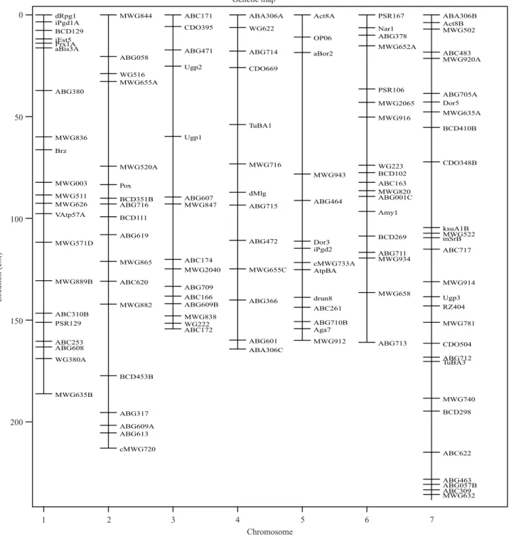
For QTL detection and for the analysis of QxE, we used the 'Harrington' x TR306 barley mapping population (Tinker et al., 1996) (Figure 1), which includes 141 genotypes and 25 environments, as well as the information on 140 phenotypes and 127 markers. Although the original phenotypic data might be replicated, we used here the mean values because the online repository contains this information only.
Following the procedure proposed by Eastment & Krzanowski (1982) for choosing the number of components in the AMMI model, three components were selected to be retained, and the AMMI3 was considered. The first IPC axis captured 19% of the sum of squares of the GxE; the second one, 15%; and the third one, 8%; the other axes are responsible for 58% of the interaction. Consequently, the AMMI model with two components explains 34% of the interaction sum of squares, and the AMMI model with three components explains 42% of this interaction. For a better visualization, the AMMI2 biplot with the first two IPC is depicted, accounting for 34% of the interaction sum of squares (Figure 2).
In the comparison of the AMMI and W-AMMI columns, the angle changes between the genotypes and the environments are more evident. For instance, the genotype 4 is recommended to the environment SK92c by the AMMI model. However, the same genotype 4 shows a strong and positive interaction with the
Figure 1. Genetic map data for the 'Harrington' x TR306 barley mapping population. change, almost imperceptible. A small reduction of the
angle between the genotype 59 and the environment
AB92c, when comparing the two biplots, illustrates
environment AB92c, when analyzing the W-AMMI columns model. Therefore, the most recommended genotype to the environment SK92c now is the number 80. We also noticed that genotypes 25 and 92 had a high correlation with the environment MB93, in the W-AMMI columns, and that these genotypes were not recommended to this environment with the AMMI model.
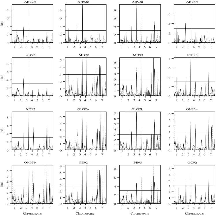
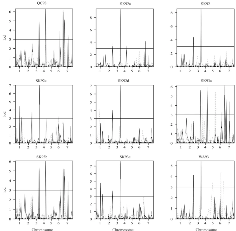
The results regarding the QxE did not consider the rows of the W-AMMI model because its predicted values are very similar to the ones by the standard AMMI model, and, therefore, their results were very similar. QTL scans to each of the 25 environments of the mapping population are presented (Figures 3 and 4 ). These figures include the QTL scans for the raw data, the QTL scans for the AMMI3 predicted values (AQ analysis), and the QTL scans for the “columns” of predicted values of W-AMMI3 (W-AQ columns). Table 1 shows the QTL detections for all environments, including the chromosome, the LOD score, and the position of the detected QTLs in the 'Harrington' x TR306 Barley mapping population, for the raw data, for the predicted values by the standard AMMI model, and for the predicted values by the W-AMMI columns model.
By analyzing the magnitude of the LOD scores in the QTL scans, we noticed a visible improvement when using the AMMI columns predicted values, not only in the number of detected QTLs, but also on the LOD scores, in comparison to the QTL scans on the raw phenotypic data and on the AMMI predicted values (AQ analysis). As expected, based on the results from Gauch et al. (2011), the QTL scans on the raw phenotypic data provide lower LOD scores than the QTL scans on the AMMI predicted values.
For instance, in the environment AK93, which was the most significantly associated with the interaction, the chromosomes 2 and 3 show QTLs only when the scan was made using the W-AMMI model. Yet, the chromosome 2 had a high-LOD score in the environment AB92b when the QTL scan was obtained with the AMMI or W-AMMI columns predicted values. The highest-LOD score values were found for the W-AMMI columns predicted values, and the biggest value was approximately 9.46 on chromosome 3, for the environment AK93.
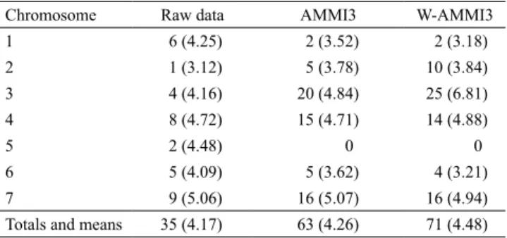
Table 1 shows the number of detected QTL per chromosome and the mean LOD scores for those Figure 2 . Biplots for the 'Harrington' x TR306 barley
detections for the raw phenotypic data, for the predicted values by the standard AMMI model, and for the predicted values by the W-AMMI columns model. The total number of detected QTL and the
mean LOD scores were bigger with the W-AMMI columns model. The possible false positive detections on the raw data, for chromosomes 1 and 5, were very few with AMMI and W-AMMI columns. Moreover,
the clear QTLs in chromosomes 3 and 7 were only detected 4 and 9 times, respectively, when considering the QTL scans of the raw data, but 20 and 16 when considering the AMMI predicted values, and 25 and
16 times, when considering the W-AMMI columns predicted values. This reinforces the idea that the QTLs obtained from the AMMI predicted values gain strength from other environments, and that the
proposed W-AMMI columns improves even further the QTL detections.
The weights for the W-AMMI algorithm can be chosen in accordance with set requirements in Smith et al. (2001), Möhring & Piepho (2009), and Welham et al. (2010). It is worth mentioning that the weights in the W-AMMI algorithm used here require a (re)scaling that leads them to values between zero and one. In specific cases with little (error) variance heterogeneity (Gauch et al., 2011), the standard AMMI model is totally appropriate. By directing the approach that will be used in a given experiment – the AMMI or W-AMMI models –, the error or residual variance for each environment should be calculated and, after that, checked for its homogeneity in all environments. If the error variance in the environments is homogeneous, the results from the AMMI model will be similar to those in the W-AMMI approach. Therefore, the AMMI standard model strategy is already sufficient. However, when the error variations have a high heterogeneity among the environments, the use of the AMMI model is not recommended, and the W-AMMI algorithm should be used (Rodrigues et al., 2014).
The techniques presented here to detect and understand GxE and QxE are based on statistical principles, with applicability in microbial and plant populations studied in various environments, and they can be adapted to genetic studies on animals and humans (Gauch et al., 2011; Rodrigues et al., 2014).
Conclusions
1. The proposed W-AMMI column algorithm is viable to analyze data that shows an heterogeneous variance, when there are not available replicates .
2. The use of the AMMI and W-AMMI models in the indicated cases improves the detection of quantitative trait loci, and provides a better understanding of the interaction between quantitative trait loci and the environment, which allows breeders to obtain a valuable information to increase crop productivity in different environments.
Acknowledgments
To Conselho Nacional de Desenvolvimento Científico e Tecnológico (CNPq), for financial support, through the project Universal-MCTI/CNPq No. 448775/2014-0.
References
ALIMI, N.A.; BINK, M.C.A.M.; DIELEMAN, J.A.; NICOLAI, M.; WUBS, M.; HEUVELINK, E.; MAGAN, J.; VOORRIPS, R.E.; JANSEN, J.; RODRIGUES, P.C.; VAN DER HEIJDEN, G.W.A.M.; VERCAUTEREN, A.; VUYLSTEKE, M.; SONG, Y.; GLASBEY, C.; BAROCSI, A.; LEFEBVRE, V.; PALLOIX, A.; VAN EEUWIJK, F.A. Genetic and QTL analyses of yield and a set of physiological traits in pepper. Euphytica, v.190, p.181-201, 2013. DOI: 10.1007/s10681-012-0767-0.
EASTMENT, H.T.; KRZANOWSKI, W.J. Cross-validatory choice of the number of components from a principal component analysis. Technometrics, v.24, p.73-77, 1982.
GAUCH JR., H.G. Statistical analysis of regional yield trials: AMMI analysis of factorial designs. Amsterdam: Elsevier, 1992. GAUCH, H.G.; RODRIGUES, P.C.; MUNKVOLD, J.D.; HEFFNER, E.L. SORRELLS, M. Two new strategies for detecting and understanding QTL x environment interactions. Crop Science, v.51, p.96-113, 2011. DOI: 10.2135/cropsci2010.04.0206. MÖHRING, J.; PIEPHO, H.-P. Comparison of weighting in two-stage analysis of plant breeding trials. Crop Science, v.49, 1977-1988, 2009. DOI: 10.2135/cropsci2009.02.0083.
PADEREWSKI, J.; GAUCH, H.G.; MADRY, W.; DRZAZGA, T.; RODRIGUES, P.C. Yield response of winter wheat to agro-ecological conditions using additive main effects and multiplicative interaction and cluster analysis. Crop Science, v.51, p.969-980, 2011. DOI: 10.2135/cropsci2010.05.0278.
PADEREWSKI, J.; RODRIGUES, P.C. The usefulness of EM-AMMI to study the influence of missin, data pattern and application to Polish post-registration winter wheat data.
Australian Journal of Crop Science, v.8, p.640-645, 2014. Table 1. Number of detected QTL per chromosome, and
the mean LOD scores (data inside partentheses) for these detections, using the raw phenotypic data, the predicted values with the standard AMMI model with three multiplicative terms, and the predicted values with the W-AMMI column model with three multiplicative terms.
Chromosome Raw data AMMI3 W-AMMI3 1 6 (4.25) 2 (3.52) 2 (3.18) 2 1 (3.12) 5 (3.78) 10 (3.84) 3 4 (4.16) 20 (4.84) 25 (6.81) 4 8 (4.72) 15 (4.71) 14 (4.88)
5 2 (4.48) 0 0
Received on April 21, 2017 and accepted on August 28, 2017
PEREIRA, D.; RODRIGUES, P.C.; MEJZA, S.; MEXIA, J.T. A comparison between joint regression analysis and the AMMI model: a case study with barley. Journal of Statistical Computation and Simulation, v.82, p.193-207, 2012a. DOI: 10.1080/00949655.2011.615839.
PEREIRA, D.G.S.; RODRIGUES, P.C.; MEJZA, I.; MEJZA, S.; MEXIA, J.T. Analyzing genotypes-by-environment interaction by curvilinear regression. Scientia Agricola, v.69, p.357-363, 2012b. DOI: 10.1590/S0103-90162012000600003.
RODRIGUES, P.C.; MALOSETTI, M.; GAUCH JR., H.G.; VAN EEUWIJK, F.A. A weighted AMMI algorithm to study genotype-by-environment interaction and QTL-by-environment interaction. Crop Science, v.54, p.1555-1570, 2014. DOI: 10.2135/ cropsci2013.07.0462.
RODRIGUES, P.C.; MONTEIRO, A.; LOURENÇO, V.M. A robust AMMI model for the analysis of genotype-by-environment data. Bioinformatics, v.32, p.58-66, 2016. DOI: 10.1093/bioinformatics/btv533.
RODRIGUES, P.C.; PEREIRA, D.G.S.; MEXIA, J.T. A comparison between Joint Regression Analysis and the Additive Main and Multiplicative Interaction model: the robustness with increasing amounts of missing data. Scientia Agricola, v.68, p.679-686, 2011. DOI: 10.1590/S0103-90162011000600012.
ROMAGOSA, I.; ULLRICH, S.E.; HAN, F.; HAYES, P.M. Use of the additive main eff ects and ointmultiplicative interaction model in QTL mapping for adaptation in barley. Theoretical and Applied Genetics, v.93, p.30-37, 1996. DOI: 10.1007/ BF00225723.
SMITH, A.; CULLIS, B.; GILMOUR, A. The analysis of crop variety evaluation date in Australia. Australian & New Zealand Journal of Statistics, v.43, p.129-145, 2001. DOI: 10.1111/1467-842X.00163.