leite et al 2016

Neotropical forest expansion during the last glacial

period challenges refuge hypothesis

Yuri L. R. Leite

, Leonora P. Costa

, Ana Carolina Loss

, Rita G. Rocha

, Henrique Batalha-Filho

, Alex C. Bastos

,

Valéria S. Quaresma

, Valéria Fagundes

, Roberta Paresque

, Marcelo Passamani

, and Renata Pardini

a_{Departamento de Ciências Biológicas, Centro de Ciências Humanas e Naturais, Universidade Federal do Espírito Santo, 29075-910, Vitória, ES, Brazil;} b_{Departamento de Biologia, Centro de Estudos do Ambiente e do Mar, Campus Universitário de Santiago, Universidade de Aveiro, 3810-193, Aveiro,} Portugal;c_{Departamento de Zoologia, Instituto de Biologia, Universidade Federal da Bahia, 40170-115, Salvador, BA, Brazil;}d_{Departamento de} Oceanografia e Ecologia, Centro de Ciências Humanas e Naturais, Universidade Federal do Espírito Santo, 29075-910, Vitória, ES, Brazil;e_Departamento de Ciências da Saúde, Centro Universitário Norte do Espírito Santo, Universidade Federal do Espírito Santo, 29932-540, São Mateus, ES, Brazil; f_{Departamento de Biologia, Universidade Federal de Lavras, 37200-000, Lavras, MG, Brazil; and}g_{Departamento de Zoologia, Instituto de Biociências,} Universidade de São Paulo, 05508-090, São Paulo, SP, Brazil

Edited by Rodolfo Dirzo, Stanford University, Stanford, CA, and approved December 10, 2015 (received for review July 2, 2015) The forest refuge hypothesis (FRH) has long been a paradigm for

explaining the extreme biological diversity of tropical forests. Accord-ing to this hypothesis, forest retraction and fragmentation durAccord-ing glacial periods would have promoted reproductive isolation and consequently speciation in forest patches (ecological refuges) sur-rounded by open habitats. The recent use of paleoclimatic models of species and habitat distributions revitalized the FRH, not by consid-ering refuges as the main drivers of allopatric speciation, but instead by suggesting that high contemporary diversity is associated with historically stable forest areas. However, the role of the emerged continental shelf on the Atlantic Forest biodiversity hotspot of eastern South America during glacial periods has been ignored in the literature. Here, we combined results of species distribution models with coalescent simulations based on DNA sequences to explore the congruence between scenarios of forest dynamics through time and the genetic structure of mammal species cooccurring in the central region of the Atlantic Forest. Contrary to the FRH predictions, we found more fragmentation of suitable habitats during the last interglacial (LIG) and the present than in the last glacial maximum (LGM), probably due to topography. We also detected expansion of suitable climatic conditions onto the emerged continental shelf during the LGM, which would have allowed forests and forest-adapted species to expand. The interplay of sea level and land distribution must have been crucial in the biogeographic history of the Atlantic Forest, and forest refuges played only a minor role, if any, in this biodiversity hotspot during glacial periods.

last glacial maximum

|

|

|

|

T

he extreme biological diversity of tropical forests has inspired

and puzzled naturalists and scientists for centuries, and the

forest refuge hypothesis (FRH) has long been one of the major

paradigms to explain it. According to the FRH, forest retraction

and fragmentation during glacial periods would have promoted

isolation and consequently allopatric speciation in forest patches,

or ecological refuges, surrounded by open habitats in the

Ama-zon (1). Although originally based on climate fluctuations in the

Pleistocene, the FRH was subsequently invoked for climate

changes irrespective of the time period (2). The FRH was also

applied to South America’s Atlantic Forest (3), one of the

top-five biodiversity hotspots on Earth (4). The FRH gained broad

acceptance during the 1980s when empirical paleoecological data

from neotropical rainforests were still lacking. Nevertheless, heavy

criticism came upon the FRH because some paleobotanical data

showed that forests had persisted throughout glacial cycles (5). As

paleoclimatic models of species and habitats became widely

used, recent studies revitalized the FRH, not by considering

refuges as the main drivers of allopatric speciation, but instead

by suggesting that high contemporary diversity and endemism

are associated with historically stable Atlantic Forest areas (6).

This hypothesis is based on the assumption that populations were

restricted to refugia within the bounds of the current observed

distribution of a species, thus disregarding paleogeography. Here,

we used coalescent simulations to test alternative demographic

models and found potentially larger past distributions. Contrary to

the refuge models, here, we show that forest specialist small mammal

populations actually expanded during the last glacial period, after the

expansion of the Atlantic Forest onto the Brazilian continental shelf,

a process that has been neglected in paleoenvironmental

recon-structions. This new idea is what we call the Atlantis Forest

hy-pothesis, in homage to Plato’s legendary continent, which was

eventually swallowed up by the sea.

We combined the results of distribution models with coalescent

simulations based on DNA sequences to explore the congruence

between scenarios of forest dynamics through time and the genetic

diversity of mammal species cooccurring in the central region of

the Atlantic Forest. First, we used climatic models to estimate

range shifts from the last interglacial (LIG) [∼120,000 y before

present (120 kybp)], through the last glacial maximum (LGM)

(∼21 kybp), to the present. For LGM simulations, we extended the

baseline climate data onto the exposed continental shelf, in

con-trast to other studies (6). Then, we used coalescent simulations to

test the genetic data for congruence with historic demographic

Significance

The tropical forests of South America are among the most di-verse and unique habitats in the world in terms of plant and animal species. One of the most popular explanations for this diversity and endemism is the idea that forests retracted and fragmented during glacial periods, forming ecological refuges, surrounded by dry lands or savannas. These historically stable forest refuges would have been responsible for maintaining the pattern of diversity and endemism observed today. Here, we show that the Atlantic Forest of eastern South America probably expanded, rather than contracted, during the last glacial period. In addition, the emerged Brazilian continental shelf played a major, yet neglected, role on the evolution of this biodiversity hotspot during the last glacial period.

Author contributions: Y.L.R.L., L.P.C., and R. Pardini designed research; Y.L.R.L., L.P.C., A.C.L., R.G.R., and R. Pardini performed research; Y.L.R.L., L.P.C., A.C.L., R.G.R., H.B.-F., V.F., R. Paresque, M.P., and R. Pardini contributed new reagents/analytic tools; A.C.L., R.G.R., and H.B.-F. analyzed data; and Y.L.R.L., L.P.C., A.C.L., R.G.R., H.B.-F., A.C.B., V.S.Q., and R. Pardini wrote the paper.

The authors declare no conflict of interest. This article is a PNAS Direct Submission.

Data deposition: The sequences reported in this paper have been deposited in the Gen-Bank database. For a list of accession numbers, seeDataset S2.

1_{To whom correspondence should be addressed. Email: yuri_leite@yahoo.com.}

This article contains supporting information online atwww.pnas.org/lookup/suppl/doi:10.

models of population fragmentation, bottlenecks, and expansions

during the LGM, the LIG, and the penultimate glacial maximum,

which corresponds to marine isotope stage 6 (MIS6) (∼160 kybp)

(7). To generate and test alternative biogeographical hypotheses,

herein we used data from five forest specialist small mammal

species, whose occurrence is restricted to forested habitats.

Con-sidering their habitat fidelity (

Table S1

), these species should

provide appropriate proxy records of forest changes through time.

Results and Discussion

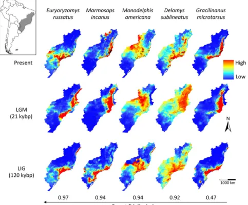
The results of species distribution models were in general

con-gruent among species, and three major trends emerged (Fig. 1).

First, species showed suitable habitat displacement toward

northern and lower elevation (i.e., warmer) areas during the

LGM. Second, we found more fragmentation of suitable habitats

during the LIG and the present than in the LGM. Third, we

detected expansion of suitable climatic conditions onto the emerged

continental shelf during the LGM, which would have allowed forests

and forest-adapted species to expand as well. The first trend is a

well-known biogeographic response to climate change, but the other

two were unexpected because they are in the opposite direction to

that predicted by the FRH, prompting us to hypothesize

alter-native biogeographic scenarios that incorporate forest expansion

during glacial periods.

We used intraspecific Bayesian coalescent simulations to

evaluate the fit of the empirical genetic data to distinct historical

scenarios (

Fig. S1

and

Tables S2

–

S6

). We first tested a single

panmictic population against subdivision into two to five

pop-ulations, either in a stable island system or including bottleneck

or expansion during the LGM. Because all scenarios of population

subdivision were rejected, we explored demographic changes in a

single panmictic population. The stability scenario was rejected for

all species, as well as bottlenecks [1–20% of the effective

pop-ulation size (N

)] in any of the three events (LGM, LIG, or MIS6)

(Fig. 2). Population expansions (1–20% of the N

) during either

LGM (which indicate population expansion onto the emerged

continental shelf) or LIG, or both, were not rejected for all forest

specialist species, usually confirming population expansion

dur-ing both LIG and LGM (Fig. 2).

The FRH posits that forest specialist species went through

cyclical population subdivision and bottlenecks during past

gla-cial periods and population stability or expansion during

inter-glacials. Our results, however, support the alternative hypothesis

that populations of forest specialist small mammals actually

ex-panded during both LIG and LGM. We therefore suggest that

the Atlantic Forest also expanded during both periods, especially

onto the exposed continental shelf during the LGM. Global sea

levels dropped to a maximum of

−150 m during Quaternary

Glacial Maxima, and the average Quaternary sea level was

around

−62 m (8). The southeastern South American coastline

thus would have been displaced hundreds of kilometers to the

east during glacial periods, exposing one of the widest shelves in

the world, the Brazilian continental shelf (9) (Fig. 3). This

ex-panded available surface area has not been taken into account in

any regional paleoecological reconstruction to date. Rather, the

area covered by Atlantic rainforest during the LGM has been

estimated at only 150,000 km

_{(excluding the continental shelf),}

which is nearly half of its current size (320,000 km

) (10). But the

shelf represents an additional 270,000 km

(9) of land available

for potential expansion. A key question, therefore, is what kind

of vegetation covered this shelf during the LGM. To address this

question, we projected modeled climatic conditions for the

At-lantic Forest and confirmed that extensive suitable areas of

broadleaf evergreen rainforest were available on the shelf during

this period (Fig. 3A), corroborating simulated LGM biome

dis-tributions based on global vegetation models (11). Analyses of a

marine sediment core from the southeastern Brazilian

conti-nental margin revealed a wide spectrum of pollen types,

in-cluding those representative of dense and semideciduous forests,

coastal scrublands, and a low frequency of grasses (12). In

con-trast, another marine core from the same region suggested

maximal grassland expansion and rainforest reduction during the

LGM (13), with the two datasets thus reflecting regional variation

in forest cover on the shelf. Other proxy data, such as changes in

the oxygen isotopic composition of planktonic foraminifera from

the same continental margin imply that maximum precipitation

actually occurred around the LGM (14), when the shelf was

ex-posed to its maximum extent. Paleochannels are also evidence of

active continental sedimentary processes along the exposed shelf

Fig. 1. Habitat suitability of Atlantic Forest small mammals through time. Modeled ranges of small mammal species sorted according to their habitat fidelity (Table S1) were projected to the present, last glacial maximum (LGM) including the exposed con-tinental shelf, and last interglacial (LIG). Habitat fidelity reflects the proportion of forest sites where each species occurs compared with open areas, ranging from 0 (lack of forest fidelity) to 1 (complete forest fidelity).

ENVIRONM

ENTAL

during low sea level periods (15), which point to the presence of

riparian forests on the shelf, further supporting our results.

Interglacial forest expansion on the continent is expected and

confirmed by a long-term (140 kybp) pollen record from the

Atlantic Forest (16). Forest extent on the continent during the

LGM is, however, a controversial topic. Pollen records suggest

that grasslands dominated south and southeastern Brazil during

this period, indicating a markedly drier and cooler climate (17),

and giving support to the FRH. In contrast, other pollen and

diatom records combined with carbon and nitrogen isotopes

suggest instead that cool, but humid, forests persisted, with no

evidence of forest retraction throughout the LGM (18). Oxygen

isotopes from speleothems, which are secondary carbonate cave

formations, also indicate wetter climate from 70 to 17 kybp,

es-pecially during the LGM (19), thus supporting the Atlantis Forest

hypothesis and refuting the FRH. We argue that, even if large

forested areas were replaced by grassland and the tree line shifted

800–1,000 m downward on the continent during glacial periods

(20), the Atlantic rainforest would have not been restricted to

small patches as predicted by the FRH because forest cover

would have extended onto the continental shelf (Fig. 3A).

The fragmentation of suitable habitats we found during both

current and previous (LIG) interglacial periods is unexpected,

given that a warmer and wetter climate is more suitable to forest

expansion. This putative fragmentation might have been the

result of topographic heterogeneity across eastern Brazil. Our

species distribution models show that, during glacial periods,

ranges are displaced to the north, where the coastal plain is very

wide and the topography is monotonously flat, allowing for

con-tinuous species ranges. During interglacials, on the other hand,

ranges moved south, where the steep coastal mountains (Serra do

Mar) drastically replace a narrow coastal plain, leading to a very

complex inland topography (Fig. 3B). The seaward side of the Serra

do Mar has the highest mean annual rainfall (up to 3,600 mm)

of the entire Atlantic Forest range whereas the inland side has

typical seasonal climates (1,300–1,600 mm) (21). This

hetero-geneous topography is associated with distinct rainfall patterns

and a mosaic of vegetation types, potentially leading to habitat

and range fragmentation.

The Atlantic Forest shows strong latitudinal differentiation,

and the geomorphological history of the continental shelf must

have played an important, yet ignored, role in this process. A

north–south floristic differentiation is caused by distinct

tem-perature and rainfall regimes as mountain ranges are

pro-gressively farther from the coast and lower in altitude to the

north of the Doce River (21) (Fig. 3B), which is a major

bio-geographic contact zone for many terrestrial vertebrate groups

(22). Furthermore, an analysis of phylogeographic endemism of

25 vertebrate species indicated that this region was recently a

location for a subdivision of the Atlantic Forest in two

bio-climatic domains (23). Rivers and river valleys are frequently

associated with biogeographic breaks in the Atlantic Forest (24),

but contrasting results raised some questions about their roles as

primary barriers whereas currently hidden geological or climatic

barriers have been invoked (25). We argue that the Brazilian

continental shelf is a putative barrier because it changes

drasti-cally at the Abrolhos Bank, from very narrow to the north to very

wide to the south, where significantly more land was exposed

during glacial periods (Fig. 3). Also, the steep slopes of the

Tubarão Bight and the Espírito Santo Mountains form one of

the narrowest lowland areas on the Brazilian coast (Fig. 3B).

This region therefore marks major geomorphological and

cli-matic transitions and must have been crucial in shaping the

evolutionary history of the adjacent biota (26). Statistical

phy-logeographic studies on other Atlantic Forest organisms showed

mixed results regarding demographic changes during the LGM,

but moderate population growth and demographic stability were

found for a warbler (27), toads (25), and one spider (28).

Eustatic changes play a major role on the evolution of islands

and coastal habitats (29, 30), but such changes have been

over-looked in the FRH debate. In addition, the vast continental shelf

has been completely ignored in paleomodeling studies of the

Atlantic Forest, despite its evolutionary significance in other

tropical areas, such as Southeast Asia, where widespread

rain-forest covered the exposed Sunda shelf during the LGM (31, 32).

These facts show that the predominantly glacial Quaternary

environment is the norm, characterized by cooler climate,

sig-nificantly lower sea levels, and slightly reduced precipitation,

which was still enough to keep large stretches of rainforest

in-stead of small refugia. This greatly expanded land area, resulting

from the exposure of the continental shelf, supported widespread

forests (31, 33). The current high sea level condition is therefore

the exception, reflecting in reduced forest area in Southeast Asia

and the Brazilian Atlantic coast. Our results show that the

in-terplay of sea level and land distribution has been crucial in the

biogeographic history of the Atlantic Forest and that forest

refuges may have played only a minor role, if any, in this

bio-diversity hotspot during glacial periods.

Materials and Methods

Selection of Taxa. Five species of small mammals, three didelphid marsupials [Marmosops incanus (Lund), Monodelphis americana (Müller), and Gracili-nanus microtarsus (Wagner)] and two cricetid sigmodontine rodents [Eur-yoryzomys russatus (Wagner) and Delomys sublineatus (Thomas)], were included in this study. These small mammals are all forest specialist species, for which ecological data indicate a clear preference for forests compared with open habitats, and should respond to both current and past alterations in the distribution of the Atlantic Forest. All five species are widespread and locally abundant in most of the Atlantic Forest (34). To verify and quantify Fig. 2. Species responses to demographic scenarios of forest refuges (red)

and forest expansion (green) during climatic oscillations from 200 kybp. (A) Benthic d18_{O records reflecting changes in seawater temperature and ice} volume (7), and corresponding demographic scenarios of population bot-tleneck (BN) and/or expansion (EX) in different periods: last glacial maximum (LGM), last interglacial (LIG), and penultimate glacial maximum (MIS6). (B) Results of the coalescent simulations for each species, confirming pop-ulation expansions during both LGM and LIG. The horizontal line represents the threshold P value (0.05) for each species. Scenarios resulting in P values at or below this level were rejected (gray), and those above this level were not rejected (black). SeeFig. S1for additional scenarios tested and rejected.

forest fidelity, we used occurrence data from previous studies (35, 36), obtained through standardized samplings (i.e., using the same type, num-ber, and disposition of traps, and the same number of sampling days) in 54 sites in the Atlantic Plateau of the state of São Paulo, southeastern Brazil. The information on species occurrence is therefore comparable among the 54 sites. One third of the sites were located in continuously forested areas within one of the largest tracts of remaining Atlantic Forest. The other 36 sites were located in open, deforested areas used for agriculture (planta-tions of annual crops) within two 10,000-ha fragmented landscapes located adjacent to the sampled continuously forested areas (18 sites within a fragmented landscape containing only 10% of remaining forest, and 18 sites within a fragmented landscapes containing 50% of remaining forest). We computed the proportion of forest and open area sites where each of the five species occurred (PF and PO, respectively). We then used these pro-portions to calculate a simple index of forest fidelity (FD= PF − PO) that varies from−1 (preference for open habitats) to +1 (preference for forests), and for which a value close to zero indicates species equally well-distributed in both habitats. All five species were well distributed in continuously for-ested areas and were absent from most of the open area sites, and fidelity values ranges from 0.47 to 0.97 (Table S1). As expected from their high forest fidelity, these selected forest specialist species negatively respond to current deforestation and forest fragmentation whereas habitat generalist species do not respond or benefit from these processes (35, 37). The obtained values of forest fidelity corroborate several other ecological studies on habitat selection or preference for all five small mammal species (34). Species and Habitat Distribution Modeling. Georeferenced occurrence locali-ties of the five target species were gathered from data from museums, sci-entific articles, theses, and dissertations (38). The museum data were obtained from the online platforms SpeciesLink (splink.cria.org.br/), Global Biodiversity Information Facility (GBIF) (www.gbif.org), and Mammal Net-worked Information System (MaNIS) (manisnet.org/). The locations of the points of occurrence were verified using Google Maps (www.google.com.br/ maps), Google Earth 7.0 (www.google.com/earth/), and SpeciesLink tools (geoLoc and infoXY), and possible mislabeled coordinates were excluded. Occurrence points for each species were then compared with distribution maps from the most recent taxonomic reviews, and discrepancies were further scrutinized to remove suspicious records. In total, we used 44 points of occurrence for E. russatus, 114 for M. incanus, 29 for M. americana, 17 for D. sublineatus, and 73 for G. microtarsus, scattered throughout the study area to create the suitability maps (Dataset S1). To estimate historical broadleaf evergreen rainforest occurrence, we used 395 points (Dataset S1) randomly extracted from the extent of this vegetation (39). To prevent

spatial autocorrelation, only points distant at least 10 km of each other were included. To estimate habitat suitability for each species and habitat, we used 19 climate variables from WorldClim (40) in the 2.5-min resolution (www.worldclim.org/). For each species and habitat, correlated environment variables were rejected, as indicated by principal component analysis (PCA) and Mantel tests conducted in R 3.0.1 (41). Climatic layers were cropped to the Atlantic Forest river basins that encompass the distribution of the target species: Paraná, South Atlantic, Southeastern Atlantic, East Atlantic, and São Francisco. The algorithm chosen for modeling was that of maximum en-tropy, as implemented in MaxEnt 3.3.3 (42). Models were run with default regularization and 10 replicates subsampled, using 20% of the points for test and 80% for training each replicate. To determine whether the model’s discrimination capacity is better than random chance, models were validated by accessing area under the curve (AUC), sensitivity, specificity, and accuracy values averaged across the replicates. The adequate environment conditions for each species and habitat in the present were projected into past layers by creating suitability maps for the last glacial maximum (LGM) period 21,000 y ago (including the continental shelf) and for the last interglacial (LIG) period 120,000 y ago. We used General Circulation Models (GCMs) for LIG and LGM estimated by the Community Climate System Model (CCSM). To estimate broadleaf evergreen rainforest occurrence during the LGM, we also used GCMs estimated by the Model for Interdisciplinary Research on Climate-Earth System Model (MIROC-ESM) and the Max-Planck-Institute Climate-Earth Sys-tem Model running in low resolution grid and paleo mode (MPI-ESM-P). All layers of bioclimatic variables are available at the WorldClim website (www. worldclim.org/). We created binary maps of broadleaf evergreen rainforest by estimating the presence/absence of suitable areas using a 10th percentile training presence logistic threshold.

DNA Extraction, Amplification, and Sequencing. Genomic DNA was isolated from tissue samples (muscle or liver samples) preserved in ethanol (Dataset S2) using the salt extraction method (43). For each species, we sampled between 13 and 30 localities and between 1 and 15 specimens per locality. Polymerase chain reactions (PCRs) were performed to amplify 801 base pairs (bp) of the Cytochrome b gene (Cyt b), using primers MVZ05 and MVZ16 (44). PCR (12.5μL) contained 1.25 μL of 10× buffer, 0.5 μL of MgCl2(50 mM), 0.25μL of dNTP solution (10 mM per nucleotide), 0.15 μL of each primer (10 mM), 0.15μL of Taq Platinum (Invitrogen Life Technologies), and 1 μL of DNA (20 ng/μL). The PCR profile was as follows: initial denaturation at 94 °C for 5 min, followed by 39 cycles at 94 °C for 30 s, 48 °C for 45 s, 72 °C for 45 s, and a final extension at 72 °C for 5 min. PCR products were purified using ExoSAP enzymes (GE Healthcare Life Sciences), and the cycle-sequencing reactions were performed with a Big Dye v3.1 kit (Applied Biosystems Inc.), following Fig. 3. Connections between the Brazilian conti-nental shelf and the Atlantic Forest. (A) Projected extent of suitable broadleaf evergreen rainforest areas (green) during the last glacial maximum (LGM) and the present. The LGM map shows the overlap of three models (dark green), two models (medium green), and one model (light green). Suitable areas for rainforest on the continental shelf during the LGM (green) are submersed in the present (blue). (B) Topographic map of the eastern Brazilian coast emphasizing the continental shelf (light blue, bounded by the−150 m isobath) and four key fea-tures mentioned in the text: the Abrolhos Bank (site 1), Tubarão Bight (site 2), Doce River (site 3), and Espírito Santo Mountains (site 4). The lowlands (<500 m) are represented in green, the highlands (>500 m) in orange, and ocean depth increases progressively toward darker blue areas.

ENVIRONM

ENTAL

the manufacturer’s protocol. Samples were sequenced in both directions using automated DNA sequencer ABI 3500 (Thermo Fisher Scientific, Applied Biosystems), with the same primers listed above. Electropherograms were inspected, and sequences were aligned using the CLUSTAL W method imple-mented in MEGA 6 (45). All alignments were inspected and corrected manually. All generated sequences have been deposited in GenBank (Dataset S2). Summary Statistics. Newly generated and GenBank sequences were used to estimate summary statistics for each target species. Numbers of haplotypes (h), polymorphic sites (S), haplotype diversity (Hd), and nucleotide diversity (Π) for each species were estimated with DnaSP v.5 (46). Deviation from neutrality was tested through different statistics: D (47), Fs (48), and R2(49), mismatch distribution, and raggedness (50), which were calculated using DnaSP v.5. Coalescent simulations with 1,000 replicates were applied to determine the P value of each statistics. Significant P values (<0.05) were taken as evidence of demographic expansion (Table S2). These summary statistics were further used in coalescent simulations, to test the fit of each simulated scenario to observed data.

Substitution Rate Estimation. To estimate substitution rates for five taxa to be used in subsequent analyses, we used a fossil-calibrated approach (51). Es-timates were performed independently for marsupials and for rodents. Both estimates were implemented in BEAST 2.1.3 (52) assuming a Yule speciation model and using a relaxed molecular clock with lognormal distribution. For marsupials, we used a Cyt b matrix containing previously published se-quences (Table S3) and a published phylogeny (53) to set monophyletic constraints. We used two calibration points: the diversification of Didelphi-dae and the diversification of Didelphimorphia (Table S4). These calibration points were set as minimum and maximum ages, being the minimum age of the oldest unequivocal fossil belonging to clade (54). The maximum age of Didelphidae was based on stratigraphic bounding, which encompasses two stratigraphic units without fossil records of this clade (54). The maximum age of Didelphimorphia was based on phylogenetic bounding, which encompasses the age of the stem of didelphimorph (Peradectes) (54, 55). For rodents, we also used a Cyt b matrix containing previously published sequences (Table S3) and followed a published phylogeny (56) to set monophyletic constraints. We used six calibration points that represent multiple shallow (e.g., genera) and deep (e.g., tribes) calibrations of sigmodontines (56, 57) (Table S4). These calibration points were set as lognormal prior distributions, where fossil ages were set as offsets, and mean and SD were set as 1 (57). We performed two independent runs of 100,000,000 generations each and sampled every 10,000 generations. Analyses were performed in the CIPRES Science Gateway (https://www.phylo. org). Convergence of the Markov Chain Monte Carlo (MCMC) chains was verified in Tracer v.1.6 (58), making sure that all effective sample size (ESS) values were higher than 200. The resulting trees were combined using Log-Combiner, and the consensus tree was generated in TreeAnotator, after a burn-in of 10%. Consensus trees were visualized in FigTree 1.4. The sub-stitution rates obtained for each species were further used to estimate time to the most recent common ancestor (tMRCA) and in the coalescent simulations. Divergence Time Estimation. The tMRCAwas estimated independently for each of five taxa, using all available sequences of each species (Dataset S2) and two close outgroups. Before this estimation, we tested the molecular clock for each dataset by performing maximum likelihood (ML) analyses in MEGA 6. The ML values of the obtained topologies were compared with and without molecular clock constraints also using MEGA 6. We rejected the presence of a strict mo-lecular clock for the five small mammal species and used relaxed momo-lecular clock approaches in the all of the subsequent analyses. The time to the most recent common ancestor (tMRCA) for each species was estimated assuming a Yule spe-ciation model. We used a relaxed molecular clock with lognormal distribution as indicated by ML tests, our estimation of the mean substitution rates as the clock

rate, and evolution models as selected using MrModeltest (59) for each species (Table S5). To obtain absolute dates in this analysis, we used our estimation of the mean substitution rates for each species (Table S5). Estimates were imple-mented in BEAST 2.1.3 and ran in the CIPRES Science Gateway. Runs and MCMC chain convergence, as well as resulting consensus trees, were defined as de-scribed above. Mean divergence dates and 95% highest posterior densities (HPDs) were obtained from the deepest node of the species in the tree. Hypotheses Tests of Historical Scenarios. To test putative scenarios of pop-ulation diversification, we implemented coalescent simpop-ulations in the Bayesian Serial SimCoal (BayeSSC) (60, 61), and we then evaluated the fit of the empirical genetic data to distinct historical models. To evaluate fitting of each simulated scenario to the empirical data (summary statistics: h, S,Π, Tajima’s D, and pairwise differences), we applied the statistical framework described in the literature (27, 62–65). We started with simple models as a baseline against which more complex ones were compared (66). First, we simulated a scenario of a single panmictic population without any de-mographic event throughout time, which was then compared with three population subdivision models, where the ancestral population was sepa-rated into two, three, and five subpopulations (Fig. S1). The subdivision date was based on the estimates of tMRCAof each species (Table S5). We then simulated bottlenecks and expansions during the last glacial maximum (LGM) [∼11,000–33,000 y before present (11–33 kybp)], the last interglacial (LIG) (∼109–130 kybp), and the penultimate glacial period, which corre-sponds to marine isotope stage 6 (MIS6) (∼130–185 kybp) (67, 68). Bottle-necks and expansions were first simulated for each period separately and were then conjugated in both LGM and LIG (Fig. S1). These demographic events were simulated to reduce or increase the population effective size (Ne) to 1–10% and 5–20% of the current size (under a uniform prior). To further test a scenario of broader expansion, we also simulated an increase of 30–50% (under a uniform prior) during LIG followed by an increase of 5–20% (under a uniform prior) during the LGM. Newas estimated from theta (Θ), according to the following formula: Θ = 2μNe, whereμ is the mutation rate previously obtained for each species (Table S5).Θ was estimated in MIGRATE-N 3.6 (69) using transition/transversion ratios for each species es-timated in MEGA 6 (Table S5), a static heating scheme, and the Bayesian Inference option with the default search parameters. For population sub-division models, we assumed that Nefrom each present population was 1/2, 1/3, and 1/5 of the species Ne. In these scenarios, we assumed a linear stepping-stone model, with migration (m) equal to 0.01. BayeSSC input files for each species included the estimated range of population effective size Ne (under a uniform prior), mutation rates, generation time of 1 y (70), and transition/transversion (T/T) ratios (Table S5). For each model, we ran 1,000 simulations, in which five simulated summary statistics were obtained (h, S, Π, Tajima’s D, and pairwise differences). These simulations were then tested against observed data for each species (71). For assessing the significance of our data, we followed the procedure described in the literature (62, 63), where each summary statistic was compared with values representing the empirical distribution of the statistic from simulation. We then compared the combined empirical likelihood of each summary statistic (Cobs) against a null distribution of C (62, 63) and rejected simulated scenarios when P≤ 0.05 (Table S6).

ACKNOWLEDGMENTS. We thank J. Justino, L. Zanchetta, J. Dalapicolla, J. Agrizzi, R. Guimarães, R. Duda, and the many undergraduate students for laboratory work. We thank J. L. Patton and A. B. Rylands for helpful discus-sions and advice; M. Nascimento, J. Guedes, V. Colombi, V. Vale, E. Guerra, R. Duda, and K. Alves for field assistance; and J. Hoppe and F. Barreto for assistance with distribution models. This study was funded by Fundação de Amparo à Pesquisa e Inovação do Espírito Santo (FAPES, Brazil) and Conselho Nacional de Desenvolvimento Científico e Tenológico (CNPq, Brazil).

1. Haffer J (1969) Speciation in amazonian forest birds. Science 165(3889):131–137. 2. Haffer J (1997) Alternative models of vertebrate speciation in Amazonia: An

over-view. Biodivers Conserv 6:451–476.

3. Prance GT (1982) Biological Diversification in the Tropics (Columbia Univ Press, New York). 4. Myers N, Mittermeier RA, Mittermeier CG, da Fonseca GAB, Kent J (2000) Biodiversity

hotspots for conservation priorities. Nature 403(6772):853–858.

5. Colinvaux P, de Oliveira P, Moreno J, Miller M, Bush M (1996) A long pollen record from lowland Amazonia: Forest and cooling in glacial times. Science 274:85–88. 6. Carnaval AC, Moritz C (2008) Historical climate modeling predicts patterns of current

biodiversity in the Brazilian Atlantic forest. J Biogeogr 35:1187–1201.

7. Cohen KM, Gibbard P (2011) Global Chronostratigraphical Correlation Table for the Last 2.7 Million Years (Subcommission on Quaternary Stratigraphy, International Commission on Stratigraphy, Cambridge). Available at quaternary.stratigraphy.org/ charts. Accessed June 30, 2015.

8. Rabineau M, et al. (2006) Paleo sea levels reconsidered from direct observation of paleoshoreline position during Glacial Maxima (for the last 500,000 yr). Earth Planet Sci Lett 252:119–137.

9. Nagai RH, Sousa SHM, Mahiques MM (2014) The southern Brazilian shelf. Continental Shelves of the World: Their Evolution During the Last Glacio-Eustatic Cycle, eds Chiocci FL, Chivas AR (Geological Society Memoirs, London), pp 47–54.

10. Behling H (2002) Carbon storage increases by major forest ecosystems in tropical South America since the Last Glacial Maximum and the early Holocene. Global Planet Change 33:107–116.

11. Prentice IC, Harrison SP, Bartlein PJ (2011) Global vegetation and terrestrial carbon cycle changes after the last ice age. New Phytol 189(4):988–998.

12. Freitas AG, Carvalho MA, Mendonça CBF, Gonçalves-Esteves V (2013) Pollen grains in Quaternary sediments from the Campos Basin, state of Rio de Janeiro, Brazil: Core BU-91-GL-05. Acta Bot Brasilica 27:761–772.

13. Behling H, Arzb HW, Pätzold J, Wefer G (2002) Late Quaternary vegetational and climate dynamics in southeastern Brazil, inferences from marine cores GeoB 3229-2 and GeoB 3202-1. Palaeogeogr Palaeoclimatol Palaeoecol 179:227–243.

14. Pivel MAG, Toledo FAL, Costa KB (2010) Foraminiferal record of changes in summer monsoon precipitation at the southeastern Brazilian continental margin since the Last Glacial Maximum. Revista Brasileira de Paleontologia 13:79–88.

15. Dominguez JML, da Silva RP, Nunes AS, Freire AFM (2013) The narrow, shallow, low-accommodation shelf of central Brazil: Sedimentology, evolution, and human uses. Geomorphology 203:46–59.

16. Ledru MP, Mourguiart P, Riccomini C (2009) Related changes in biodiversity, in-solation and climate in the Atlantic rainforest since the last interglacial. Palaeogeogr Palaeoclimatol Palaeoecol 271:140–152.

17. Behling H (2002) South and southeast Brazilian grasslands during Late Quaternary times: A synthesis. Palaeogeogr Palaeoclimatol Palaeoecol 177:19–27.

18. Pessenda LCR, et al. (2009) The evolution of a tropical rainforest/grassland mosaic in southeastern Brazil since 28,000 14C yr BP based on carbon isotopes and pollen re-cords. Quat Res 71:437–452.

19. Cruz FW, et al. (2009) Orbital and millennial-scale precipitation changes in Brazil from speleothem records. Past Climate Variability in South America and Surrounding 29 Regions: From the Last Glacial Maximum to the Holocene, eds Vimeux F, Sylvestre F, Khodri M (Springer, Dordrecht, The Netherlands), pp 29–60.

20. Behling H (2008) Tropical mountain forest dynamics in Mata Atlantica and northern Andean biodiversity hotspots during the late Quaternary. The Tropical Mountain Forest: Patterns and Processes in a Biodiversity Hotspot, eds Gradstein SR, Homeier J, Gansert D (Universitätsverlag Göttingen, Göttingen, Germany), pp 25–33.

21. Oliveira-Filho AT, Fontes MA (2000) Patterns of floristic differentiation among Atlantic forests in Southeastern Brazil and the influence of climate. Biotropica 32:793–810. 22. Costa LP, Leite YLR (2013) Historical fragmentation shaping vertebrate diversification

in the Atlantic Forest biodiversity hotspot. Bones, Clones, and Biomes: The History and Geography of Recent Neotropical Mammals, eds Patterson BD, Costa LP (Chicago Univ Press, Chicago), pp 283–306.

23. Carnaval AC, et al. (2014) Prediction of phylogeographic endemism in an environ-mentally complex biome. Proc Biol Sci 281(1792):20141461.

24. Pellegrino KCM, et al. (2005) Phylogeography and species limits in the Gymnodactylus darwinii complex (Gekkonidae, Squamata): Genetic structure coincides with river systems in the Brazilian Atlantic Forest. Biol J Linn Soc Lond 85:13–26.

25. Thomé MTC, Zamudio KR, Haddad CFB, Alexandrino J (2014) Barriers, rather than refugia, underlie the origin of diversity in toads endemic to the Brazilian Atlantic Forest. Mol Ecol 23(24):6152–6164.

26. Pereira TL, et al. (2013) Dispersal and vicariance of Hoplias malabaricus (Bloch, 1794) (Teleostei, Erythrinidae) populations of the Brazilian continental margin. J Biogeogr 40:905–914. 27. Batalha-Filho H, Cabanne GS, Miyaki CY (2012) Phylogeography of an Atlantic forest

passerine reveals demographic stability through the last glacial maximum. Mol Phylogenet Evol 65(3):892–902.

28. Peres EA, et al. (2015) Pleistocene niche stability and lineage diversification in the subtropical spider Araneus omnicolor (Araneidae). PLoS One 10(4):e0121543. 29. Ali JR, Aitchison JC (2014) Exploring the combined role of eustasy and oceanic island

thermal subsidence in shaping biodiversity on the Galápagos. J Biogeogr 41:1227–1241. 30. Huntley B, Allen JRM, Barnard P, Collingham YC, Holliday PR (2013) Species distri-bution models indicate contrasting late-Quaternary histories for Southern and Northern Hemisphere bird species. Glob Ecol Biogeogr 22:277–288.

31. Wang XM, Sun XJ, Wang PX, Stattegger K (2009) Vegetation on the Sunda Shelf, South China Sea, during the Last Glacial Maximum. Palaeogeogr Palaeoclimatol Palaeoecol 278:88–97. 32. Raes N, et al. (2014) Historical distribution of Sundaland’s Dipterocarp rainforests at

Quaternary glacial maxima. Proc Natl Acad Sci USA 111(47):16790–16795. 33. Cannon CH, Morley RJ, Bush ABG (2009) The current refugial rainforests of Sundaland

are unrepresentative of their biogeographic past and highly vulnerable to distur-bance. Proc Natl Acad Sci USA 106(27):11188–11193.

34. Rossi NF (2011) Non-volant small mammals of the Atlantic Plateau of São Paulo: Identification, natural history and threats. Master’s thesis (Universidade de São Paulo, São Paulo, Brazil). Available at www.teses.usp.br/teses/disponiveis/41/41133/tde-21092011-091459/pt-br.php. Accessed June 30, 2015.

35. Pardini R, Bueno AdeA, Gardner TA, Prado PI, Metzger JP (2010) Beyond the frag-mentation threshold hypothesis: Regime shifts in biodiversity across fragmented landscapes. PLoS One 5(10):e13666.

36. Umetsu F (2010) Effect of landscape context at different scales on the distribution of small mammals in areas of agriculture and in forest remnants. PhD dissertation (Universidade de São Paulo, São Paulo, Brazil). Available at www.teses.usp.br/teses/ disponiveis/41/41133/tde-17112010-190713/pt-br.php. Accessed June 30, 2015. 37. Banks-Leite C, et al. (2014) Using ecological thresholds to evaluate the costs and

benefits of set-asides in a biodiversity hotspot. Science 345(6200):1041–1045. 38. Alves KS (2013) Padrões de distribuição de pequenos mamíferos não-voadores na

Mata Atlântica do Brasil e variáveis ambientais associadas. Master’s thesis (Uni-versidade Federal do Espírito Santo, Vitória, Brazil).

39. IBGE (1998) Mapa da Vegetação do Brasil (Fundação Instituto Brasileiro de Geografia Estatística, Rio de Janeiro).

40. Hijmans RJ, Cameron SE, Parra JL, Jones PG, Jarvis A (2005) Very high resolution in-terpolated climate surfaces for global land areas. Int J Climatol 25:1965–1978. 41. R Development Core Team (2011) R: A Language and Environment for Statistical

Com-puting (R Foundation for Statistical ComCom-puting, Vienna). Available at www.R-project.org. 42. Phillips SJ, Anderson RP, Schapire RE (2006) Maximum entropy modeling of species

geographic distributions. Ecol Modell 190:231–259.

43. Bruford MW, Hanotte O, Brookfield JFY, Burke T (1992) Single-locus and DNA fin-gerprinting. Molecular Genetic Analyses of Populations: A Practical Approach, ed Hoelzel AR (IRL Press, Oxford), pp 225–269.

44. Smith MF, Patton JL (1993) The diversification of South American murid rodents: Evidence from mitochondrial DNA sequence data for the akodontine tribe. Biol J Linn Soc Lond 50:149–177.

45. Tamura K, Stecher G, Peterson D, Filipski A, Kumar S (2013) Mega 6: Molecular evo-lutionary genetics analysis version 6.0. Mol Biol Evol 30(12):2725–2729.

46. Librado P, Rozas J (2009) DnaSP v5: A software for comprehensive analysis of DNA polymorphism data. Bioinformatics 25(11):1451–1452.

47. Tajima F (1989) Statistical method for testing the neutral mutation hypothesis by DNA polymorphism. Genetics 123(3):585–595.

48. Fu YX (1997) Statistical tests of neutrality of mutations against population growth, hitchhiking and background selection. Genetics 147(2):915–925.

49. Ramos-Onsins SE, Rozas J (2002) Statistical properties of new neutrality tests against population growth. Mol Biol Evol 19(12):2092–2100.

50. Harpending HC (1994) Signature of ancient population growth in a low-resolution mitochondrial DNA mismatch distribution. Hum Biol 66(4):591–600.

51. Ho SYW, Phillips MJ (2009) Accounting for calibration uncertainty in phylogenetic estimation of evolutionary divergence times. Syst Biol 58(3):367–380.

52. Bouckaert R, et al. (2014) BEAST 2: A software platform for Bayesian evolutionary analysis. PLoS Comput Biol 10(4):e1003537.

53. Voss RS, Jansa SA (2009) Phylogenetic Relationships and Classification of Didelphid Marsupials, an Extant Radiation of New World Metatherian Mammals (American Museum of Natural History, New York), Bulletin No. 322.

54. Meredith RW, et al. (2011) Impacts of the Cretaceous terrestrial revolution and KPg extinction on mammal diversification. Science 334(6055):521–524.

55. Horovitz I, et al. (2009) Cranial anatomy of the earliest marsupials and the origin of opossums. PLoS One 4(12):e8278.

56. Leite RN, et al. (2014) In the wake of invasion: Tracing the historical biogeography of the South American cricetid radiation (Rodentia, Sigmodontinae). PLoS One 9(6):e100687. 57. Leite YLR, Kok PJR, Weksler M (2015) Evolutionary affinities of the“Lost World” mouse suggest a late Pliocene connection between the Guiana and Brazilian shields. J Biogeogr 42:706–715.

58. Rambaut A, Drummond AJ (2013) Tracer (University of Edinburgh, Edinburgh), Ver-sion 1.6. Available at beast.bio.ed.ac.uk/Tracer.

59. Nylander JAA (2004) MrModeltest (Uppsala University, Uppsala), Version 2. Available at https://github.com/nylander/MrModeltest2.

60. Excoffier L, Novembre J, Schneider S (2000) SIMCOAL: A general coalescent program for the simulation of molecular data in interconnected populations with arbitrary demography. J Hered 91(6):506–509.

61. Anderson CNK, Ramakrishnan U, Chan YL, Hadly EA (2005) Serial SimCoal: A pop-ulation genetics model for data from multiple poppop-ulations and points in time. Bioinformatics 21(8):1733–1734.

62. Voight BF, et al. (2005) Interrogating multiple aspects of variation in a full re-sequencing data set to infer human population size changes. Proc Natl Acad Sci USA 102(51):18508–18513.

63. Fabre V, Condemi S, Degioanni A (2009) Genetic evidence of geographical groups among Neanderthals. PLoS One 4(4):e5151.

64. Maldonado-Coelho M, Blake JG, Silveira LF, Batalha-Filho H, Ricklefs RE (2013) Rivers, refuges and population divergence of fire-eye antbirds (Pyriglena) in the Amazon Basin. J Evol Biol 26(5):1090–1107.

65. Cabanne GS, Sari EHR, Meyer D, Santos FR, Miyaki CY (2013) Matrilineal evidence for demographic expansion, low diversity and lack of phylogeographic structure in the Atlantic forest endemic Greenish Schiffornis Schiffornis virescens (Aves: Tityridae). J Ornithol 154:371–384.

66. Nielsen R, Beaumont MA (2009) Statistical inferences in phylogeography. Mol Ecol 18(6):1034–1047.

67. Lisiecki LE, Raymo MEA (2005) Pliocene-Pleistocene stack of 57 globally distributed benthic d18_{O records. Paleoceanography 20:PA1003.}

68. Roucoux KH, Tzedakis PC, Lawson IT, Margari V (2011) Vegetation history of the penultimate glacial period (Marine Isotope Stage 6) at Ioannina, north-west Greece. J Quat Sci 26:616–626.

69. Beerli P, Palczewski M (2010) Unified framework to evaluate panmixia and migration direction among multiple sampling locations. Genetics 185(1):313–326.

70. Pacifici M, et al. (2013) Generation length for mammals. Nat Conserv 5:87–94. 71. Hickerson MJ, Dolman G, Moritz C (2006) Comparative phylogeographic summary

statistics for testing simultaneous vicariance. Mol Ecol 15(1):209–223.

72. Marshall LG (1976) New didelphine marsupials from the La Venta fauna (Miocene) of Colombia, South America. J Paleontol 50:402–418.

73. Jacobs LL, Lindsay EH (1981) Prosigmodon oroscoi, a new sigmodont rodent from the Late Tertiary of Mexico. J Paleontol 55:425–430.

74. Peláez-Campomanes P, Martin RA (2005) The Pliocene and Pleistocene history of cotton rats in the Meade basin of southwestern Kansas. J Mammal 86:475–494. 75. Pardiñas UFJ, D’Elía G, Ortiz PE (2002) Sigmodontinos fósiles (Rodentia, Muroidea,

Sigmodontinae) de América del Sur: Estado actual de su conocimiento y prospectiva. Mastozool Neotrop 9:209–252.

76. Reig OA (1978) Roedores cricétidos del Plioceno superior de la provincia de Buenos Aires (Argentina). Publ Mus Municip Cienc Natur Lorenzo Scaglia 2:164–190. 77. Pardiñas UFJ, Tonni EP (1998) Procedencia estratigráfica y edad de los más antiguos

muroideos (Mammalia, Rodentia) de América del Sur. Ameghiniana 35:473–475. 78. Voglino D, Pardiñas UFJ (2005) Roedores sigmodontinos (Mammalia: Rodentia:

Cri-cetidae) y otros micromamíferos pleistocénicos del norte de la provincia de Buenos Aires (Argentina): Reconstrucción paleoambiental para el Ensenadense cuspidal. Ameghiniana 42:143–158.

79. Pardiñas UFJ, Teta P, Voglino D, Fernandez FJ (2013) Enlarging rodent diversity in westcentral Argentina: A new species of the genus Holochilus (Cricetidae, Sigmodontinae). J Mammal 94:231–240.

ENVIRONM

ENTAL