CPD
9, 3519–3561, 2013D-O Boreal CH4
emissions
P. O. Hopcroft et al.
Title Page
Abstract Introduction
Conclusions References
Tables Figures
◭ ◮
◭ ◮
Back Close
Full Screen / Esc
Printer-friendly Version
Interactive Discussion
Discussion
P
a
per
|
D
iscussion
P
a
per
|
Discussion
P
a
per
|
Discuss
ion
P
a
per
|
Clim. Past Discuss., 9, 3519–3561, 2013 www.clim-past-discuss.net/9/3519/2013/ doi:10.5194/cpd-9-3519-2013
© Author(s) 2013. CC Attribution 3.0 License.
Open Access
Climate of the Past
Discussions
Geoscientiic Geoscientiic
Geoscientiic Geoscientiic
This discussion paper is/has been under review for the journal Climate of the Past (CP). Please refer to the corresponding final paper in CP if available.
Limited response of peatland CH
4
emissions to abrupt Atlantic Ocean
circulation changes in glacial climates
P. O. Hopcroft1, P. J. Valdes1, R. Wania2, and D. J. Beerling3
1
Bristol Research Initiative for the Dynamic Global Environment (BRIDGE), School of Geographical Sciences, University of Bristol, Bristol BS8 1SS, UK 2
Lanser Strasse 30, 6080 Igls, Austria 3
Department of Animal and Plant Sciences, University of Sheffield, Sheffield S10 2TN, UK
Received: 23 May 2013 – Accepted: 13 June 2013 – Published: 26 June 2013
Correspondence to: P. O. Hopcroft ([email protected])
CPD
9, 3519–3561, 2013D-O Boreal CH4
emissions
P. O. Hopcroft et al.
Title Page
Abstract Introduction
Conclusions References
Tables Figures
◭ ◮
◭ ◮
Back Close
Full Screen / Esc
Printer-friendly Version
Interactive Discussion
Discussion
P
a
per
|
D
iscussion
P
a
per
|
Discussion
P
a
per
|
Discuss
ion
P
a
per
|
Abstract
Ice-core records show that abrupt Dansgaard-Oeschger climatic warming events of the last glacial period were accompanied by large increases in the atmospheric CH4
con-centration (up to 200 ppbv). These abrupt changes are generally regarded as arising from the effects of changes in the Atlantic Ocean meridional overturning circulation
5
and the resultant climatic impact on natural CH4 sources, in particular wetlands. We
use two different ecosystem models of wetland CH4 emissions to simulate northern CH4 sources forced with coupled general circulation model simulations of five diff
er-ent time periods during the last glacial to investigate the poter-ential influence of abrupt ocean circulation changes on atmospheric CH4 levels during D-O events. The
simu-10
lated warming over Greenland of 7–9◦C in the different time-periods is at the lower end of the range of 11–15◦C derived from ice-cores, but is associated with strong im-pacts on the hydrological cycle, especially over the North Atlantic and Europe during winter. We find that although the sensitivity of CH4emissions to the imposed climate
varies significantly between the two ecosystem emissions models, the model
simula-15
tions do not reproduce sufficient emission changes to satisfy ice-core observations of CH4 increases during abrupt events. This suggests that alternative scenarios of
cli-matic change could be required to explain the abrupt glacial CH4variations.
1 Introduction
Dansgaard-Oeschger (D-O) cycles are chiefly characterised by a series of 25 incredibly
20
abrupt warming episodes which occurred during the last glacial period. These events have been reconstructed from Greenland ice-core data (e.g. NGRIP Project Members, 2004; Wolffet al., 2010) and from an increasing number of palaeoclimate proxies from across the globe (e.g. Peterson et al., 2000; Hendy and Kennett, 2000; Wang et al., 2001; Kanner et al., 2012). D-O events typically constitute abrupt warmings of 8 to
25
CPD
9, 3519–3561, 2013D-O Boreal CH4
emissions
P. O. Hopcroft et al.
Title Page
Abstract Introduction
Conclusions References
Tables Figures
◭ ◮
◭ ◮
Back Close
Full Screen / Esc
Printer-friendly Version
Interactive Discussion
Discussion
P
a
per
|
D
iscussion
P
a
per
|
Discussion
P
a
per
|
Discuss
ion
P
a
per
|
temperature transitions were also accompanied by abrupt changes in atmospheric CH4, N2O, dust andδD of ice (e.g. Huber et al., 2006; Wolffet al., 2010), suggesting
large-scale abrupt climatic changes which present a challenge to our understanding of natural climatic variability (Seager and Battisti, 2007).
At present D-O climate events are poorly understood and there remain a number of
5
different hypotheses of their causation (e.g. Clement and Peterson, 2008; Liu et al., 2009; Li et al., 2010; Petersen et al., 2013). The predominant theory revolves around non-linear changes in the deep-water formation in the North Atlantic Ocean associ-ated with the Atlantic meridional overturning circulation (AMOC) and its Northwards heat transport. Abrupt climate transitions in a glacial state have been demonstrated
10
in intermediate complexity climate models (e.g. Ganopolski and Rahmstorf, 2001), but the behaviour in fully coupled general circulation models appears fundamentally diff er-ent (Liu et al., 2009), relating to changes in the strength of the AMOC rather than the latitudinal position. This is potentially as a result of the inclusion of feedbacks from a dynamic atmospheric model (Yin et al., 2006).
15
Atmospheric CH4 is one of the few quantities recorded in Greenland ice (Flückiger
et al., 2004; Spahni et al., 2005) which suggests widespread climatic anomalies during D-O events, and it potentially provides quantitative constraints on the nature of D-O events. Ice-core data show that CH4shifts during D-O warming events are large,
rang-ing up to two thirds of the glacial-interglacial (G-IG) range, i.e. rapid increases of up to
20
200 ppbv (Huber et al., 2006; Flückiger et al., 2004; Wolffet al., 2010). Ice-core data on the interpolar gradient of CH4 as well as its isotopic signature allow for top-down
estimates of the changes in sources during past climate and in general suggest that wetland emissions played a significant role in past atmospheric CH4variations. Recent improvements in the determination of the interpolar gradient of CH4from ice-core mea-25
CPD
9, 3519–3561, 2013D-O Boreal CH4
emissions
P. O. Hopcroft et al.
Title Page
Abstract Introduction
Conclusions References
Tables Figures
◭ ◮
◭ ◮
Back Close
Full Screen / Esc
Printer-friendly Version
Interactive Discussion
Discussion
P
a
per
|
D
iscussion
P
a
per
|
Discussion
P
a
per
|
Discuss
ion
P
a
per
|
et al. (2000) who concluded that northern sources played a dominant role during these abrupt events.
Hopcroft et al. (2011) used the Sheffield Dynamic Global Vegetation Model (SDGVM) (Woodward et al., 1995; Beerling and Woodward, 2001) to simulate the global wet-land CH4 emission responses in a series of different climate simulations with large 5
AMOC perturbations. Globally the simulated CH4changes translated into atmospheric
increases ranging from 50 to 110 ppbv, and were considered too small to be recon-ciled with ice-core observations, especially the changes in emissions from the Northern hemisphere extra-tropics. By contrast the model has been used to successfully predict the longer orbital-scale changes in atmospheric CH4 of the last 120 kyr (Singarayer
10
et al., 2011). The weak response to abrupt changes was thought to result either from deficiencies in the climate scenario, or the sensitivity of the CH4emission model
em-ployed within SDGVM (modified from Cao et al., 1996). For example, SDGVM does not simulate the difference between air and soil temperatures. Hence it does not directly include the influence of freezing on soil moisture availability and does not include
ver-15
tical discretisation of thermodynamics in the soil which could be crucial for correctly simulating abrupt changes in CH4 emissions. Additionally, the climate simulations of Hopcroft et al. (2011) were idealised, pertaining either to the LGM (Last Glacial Max-imum: 21 kyr BP), or to some idealised boundary conditions (e.g. LGM with altered orbital insolation). This complicated the direct comparison with D-O events which show
20
great variability, especially in terms of the amplitude of abrupt CH4 rises, which are
thought to arise through the influence of longer-term changes in atmospheric CO2and
orbital insolation values (e.g. Flückiger et al., 2004).
Here we focus on the potential responses of the Northern Boreal wetlands at spe-cific time-periods relevant for understanding the D-O CH4 anomalies. We used the 25
cli-CPD
9, 3519–3561, 2013D-O Boreal CH4
emissions
P. O. Hopcroft et al.
Title Page
Abstract Introduction
Conclusions References
Tables Figures
◭ ◮
◭ ◮
Back Close
Full Screen / Esc
Printer-friendly Version
Interactive Discussion
Discussion
P
a
per
|
D
iscussion
P
a
per
|
Discussion
P
a
per
|
Discuss
ion
P
a
per
|
mates are then used to drive the dynamic vegetation model LPJ-WHyMe (Wania et al., 2009a,b, 2010) and for comparison SDGVM to simulate the response of the North-ern peatlands and permafrost to abrupt climate changes in the North Atlantic region. LPJ-WHyMe is a development of LPJ (Gerten et al., 2004) and includes representa-tions of permafrost thermodynamics and hydrology and peatland carbon cycling and
5
methane emissions. The comparison with SDGVM allows an assessment of changes to sensitivities that are caused by the presence of these additional processes as com-pared with a more generalised wetland CH4scheme. This modelling setup is used to
test assumptions about the climate- CH4 coupling of D-O warming events and to
in-vestigate the potential for constraints on mechanisms of climate change during these
10
abrupt transitions.
2 Methods
2.1 Coupled GCM simulations
We performed a series of coupled atmosphere-ocean climate model simulations using the FAMOUS coupled general circulation model (Smith et al., 2008), a low-resolution
15
version of HadCM3 (Gordon et al., 2000). The model is configured following the meth-ods of Singarayer and Valdes (2010) for the time perimeth-ods considered, which are: the LGM, 14, 38, 44 and 60 kyr, where the latter 4 are close to times of significant D-O events as shown in Table 1. In all simulations the ice sheets, land sea mask and sea-level are altered according to ICE-5G (Peltier, 2004), the CO2, CH4 and N2O mixing 20
ratios are prescribed based on Vostok and EPICA ice-core data (Petit et al., 1999; Spahni et al., 2005), and insolation is modified according to the orbital parameters of Berger and Loutre (1991). The vegetation distribution which is prescribed in FAMOUS, is based on the pre-industrial, but accounting for changes in land area and ice-sheet distribution. Each simulation is initialised from pre-industrial initial conditions and
inte-25
CPD
9, 3519–3561, 2013D-O Boreal CH4
emissions
P. O. Hopcroft et al.
Title Page
Abstract Introduction
Conclusions References
Tables Figures
◭ ◮
◭ ◮
Back Close
Full Screen / Esc
Printer-friendly Version
Interactive Discussion
Discussion
P
a
per
|
D
iscussion
P
a
per
|
Discussion
P
a
per
|
Discuss
ion
P
a
per
|
The subsequent 500 yr simulation includes a freshwater forcing scenario which is designed to produce large changes in the Atlantic meridional overturning circulation (AMOC) which drives an abrupt and large magnitude of warming over Greenland. This is consistent with previous modelling studies (e.g. Ganopolski and Rahmstorf, 2001; Liu et al., 2009; Merkel et al., 2010), though the exact mechanism of abrupt change
5
in freshwater varies between models and is not addressed here. The freshwater in-put follows that used by Hopcroft et al. (2011), and is prescribed at a maximum rate of±0.5 Sv (1 Sv=106m3s−1) over the North Atlantic between 50◦–70◦N. This forcing leads to a shutdown to essentially no overturning circulation, followed by a reasonably rapid (100 yr) change to a circulation of approximately twice the control value in each
10
time period. We also begin to explore the sensitivity to the freshwater forcing by in-cluding an additional LGM simulation with twice the magnitude (amplitude of 1.0 Sv) of freshwater forcing.
2.2 Peatland methane emission model
The peatland CH4emissions are calculated using the dynamic global vegetation model 15
LPJ-WHyMe (Lund-Potsdam-Jena Wetland Hydrology and Methane, Wania et al., 2010) which includes representations of peatland hydrology and the thermodynam-ics of permafrost to 10 m (Wania et al., 2009a,b). LPJ-WHyMe includes 2 plant func-tional types (PFTs) corresponding to C3 graminoids and Sphagnum mosses which are specific to wetlands. The carbon cycle simulated within peatland gridcells is hence
20
wetland-specific, in contrast with many previous wetland models use upland vegeta-tion distribuvegeta-tions as a proxy for the carbon balance in wetland grid-cells. CH4
emis-sions are dependent on the methanogen available carbon pool which is calculated from exudates, above- and belowground and fast and slow carbon pools, which is then weighted by root density. The temperature dependence of microbial activity is based
25
on an activation energy approach which gives more realistic behaviour at low tempera-tures compared with a formulation which employs a singleQ10 value. CH4emission by
CPD
9, 3519–3561, 2013D-O Boreal CH4
emissions
P. O. Hopcroft et al.
Title Page
Abstract Introduction
Conclusions References
Tables Figures
◭ ◮
◭ ◮
Back Close
Full Screen / Esc
Printer-friendly Version
Interactive Discussion
Discussion
P
a
per
|
D
iscussion
P
a
per
|
Discussion
P
a
per
|
Discuss
ion
P
a
per
|
LPJ-WHyMe requires monthly surface air temperatures, precipitation, cloudiness and wetdays as well as the atmospheric CO2concentration. In this work the prescribed
CO2 level generally takes the same value as in the respective FAMOUS GCM
simu-lation, and output from the transient FAMOUS experiments is used for the remaining variables, with the exception of wetdays, which is not directly simulated. We calculate
5
this field as a 12 month climatology for each model gridcell using an exponential regres-sion of the CRU observed precipitation and wetdays (1961–1990) (New et al., 1999) applied to the precipitation climatology calculated from the initial 30 yr of each model simulation.
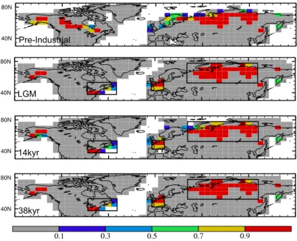
LPJ-WHyMe requires specification of the area considered peatland soils. The model
10
then interactively simulates the vegetation distribution, carbon balance, hydrology and CH4 emissions in each gridcell of peat as a function of input climate. For the
pre-industrial, this peat distribution is derived from the IGBP soil map of carbon rich north-ern soils (Wania et al., 2009a). Pre-Holocene peatland distributions can be inferred from assemblages of peat-core radiocarbon basal dates back to around 16 kyr BP. For
15
example, MacDonald et al. (2006) and Yu et al. (2010) derive time-slice maps of global peatland formation in northern areas and globally. These assemblages can then be ex-trapolated to give an estimate of the total peatland area through time, assuming linear time dependence of areal expansion around core sites (see Korhola et al., 2009 and Reyes and Cooke, 2011 for some discussion of limitations to this type of approach).
20
As a first order approach we took the current peatland areas and mapped these to palaeo-time periods taking account of land ice (Peltier, 2004) and areas of new land. This gives relatively good agreement with reconstructions (Yu et al., 2010), as this results in almost complete removal of North American and European peat areas at the LGM, although it has less impact on the Siberia peatland distribution. The total peat soil
25
sea-CPD
9, 3519–3561, 2013D-O Boreal CH4
emissions
P. O. Hopcroft et al.
Title Page
Abstract Introduction
Conclusions References
Tables Figures
◭ ◮
◭ ◮
Back Close
Full Screen / Esc
Printer-friendly Version
Interactive Discussion
Discussion
P
a
per
|
D
iscussion
P
a
per
|
Discussion
P
a
per
|
Discuss
ion
P
a
per
|
level is higher, the total area in some coastal regions of the model is smaller than at the LGM.
Sphagnum spores and peat basal dates both indicate southwards expansions of peatlands into the American Midwest and the East coast of the USA during the deglaciation between 16–12 kyr (Halsey et al., 2000; MacDonald et al., 2006). In
Eu-5
rope there is less direct pollen or core-based evidence during the deglaciation, but van Huissteden (2004) presents some evidence for the expansion of peat layers in Northern Europe during MIS 3, also a time period of abrupt shifts in atmospheric CH4. As
sen-sitivity tests, we considered two extra scenarios for each palaeo time period. The first is the complete removal of the Siberian peat complex in order to match the model peat
10
map to the late glacial distribution of Yu et al. (2010). The second involves introducing new peat gridcells in North America and Europe. Over North America, 0.35×10⁶km2 (equivalent to 35 % of the modern distribution for North America) of peatland was pre-scribed in the area South West and East the Great Lakes consistent with the areal estimate of Halsey et al. (2000) (their Fig. 8), whilst a similar area of peatland was
15
added in Northern Europe for comparison.
CH4fluxes simulated by LPJ-WHyMe must be corrected for the overestimate of mod-ern observed peatland area prescribed in the model, as well as for the effect of micro-topography which is not explicitly modelled (Spahni et al., 2011). The latter correction takes the value of 0.75, whilst the areal correction factor used here is 0.30 (c.f. 0.38 in
20
Spahni et al., 2011), giving a total peatland area in the pre-industrial of 3.20×10⁶km2 In this work for comparison purposes we also make use of the SDGVM (Sheffield Dy-namic Global Vegetation Model Woodward et al., 1995; Beerling and Woodward, 2001) which includes a generalized wetland CH4model (e.g. Valdes et al., 2005; Singarayer
et al., 2011). SDGVM uses upland PFTs to represent the carbon cycling in wetlands,
25
includes nitrogen cycling of both above- and below- ground stores and incorporates 8 soil carbon pools. In this generalized scheme, the different pathways of CH4
CPD
9, 3519–3561, 2013D-O Boreal CH4
emissions
P. O. Hopcroft et al.
Title Page
Abstract Introduction
Conclusions References
Tables Figures
◭ ◮
◭ ◮
Back Close
Full Screen / Esc
Printer-friendly Version
Interactive Discussion
Discussion
P
a
per
|
D
iscussion
P
a
per
|
Discussion
P
a
per
|
Discuss
ion
P
a
per
|
include the impact of freezing of soil water on plant water availability. The potential wetland area is calculated from the simulated soil moisture in SDGVM and emissions are calculated on monthly basis as a function of soil respiration, surface temperature, water table depth and sub-grid orography. SDGVM emissions are corrected to give the same pre-industrial total of 147 Tg CH4yr
−1
, the value used in atmospheric
chem-5
istry simulations by Valdes et al. (2005); Levine et al. (2011). This also means that the pre-industrial Northern extra-tropical flux (≥45◦N) is very similar in SDGVM and
LPJ-WHyMe. SDGVM and LPJ-WHyMe are very different in terms of processes resolved, and show different levels of sensitivity of CH4emissions to environmental factors (e.g.
Wania et al., 2013; Melton et al., 2013). The major differences between the two models
10
are summarised in Table 2.
3 Results
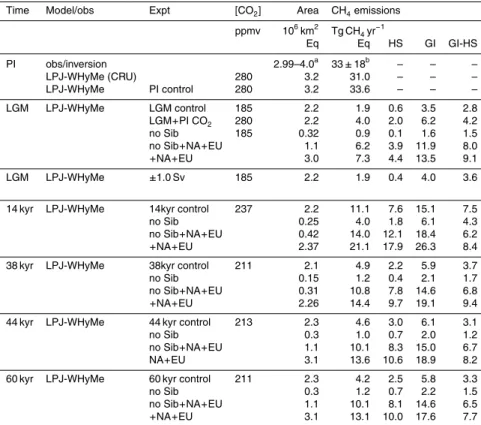
The palaeoclimate GCM simulations are summarised in Table 1 and compared with temperature anomalies derived from ice-core temperature reconstructions. FAMOUS shows more extreme cooling during the LGM and MIS3 time periods than equivalent
15
simulations with HadCM3 (Singarayer and Valdes, 2010). For example, the cooling at the LGM relative to the pre-industrial is 20◦C in FAMOUS, compared to around 14◦C in HadCM3.
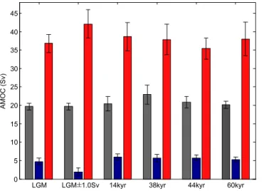
The changes in AMOC which are the principal drivers of the simulated abrupt change are shown for the 3 phases of each simulation in Fig. 1. The non-forced
20
phase (with no prescribed freshwater input) of each simulation is denoted EQ, whilst the cold and warm phases are denoted HS (Heinrich stadial) and GI (Greenland In-terstadial) respectively. These definitions are applied loosely since the climatic forc-ings which cause the oscillations observed in ice-core data are unknown. The model EQ AMOC values are relatively stable across the different time-periods at around
25
sim-CPD
9, 3519–3561, 2013D-O Boreal CH4
emissions
P. O. Hopcroft et al.
Title Page
Abstract Introduction
Conclusions References
Tables Figures
◭ ◮
◭ ◮
Back Close
Full Screen / Esc
Printer-friendly Version
Interactive Discussion
Discussion
P
a
per
|
D
iscussion
P
a
per
|
Discussion
P
a
per
|
Discuss
ion
P
a
per
|
ulations, especially when considering the considerable interannual variability as shown by the vertical bars. The only exception is the ±1.0 Sv LGM simulation for which the
HS AMOC value is weaker than the corresponding HS phases in the remaining simu-lations. In the 0.5 Sv simulations, the AMOC varies between an average HS value of around 5Sv and a GI value of 35 Sv.
5
The pattern of GI-HS warming is shown in Fig. 2 for the annual mean for 4 of the sim-ulations. The patterns in the remaining time-periods are similar to those of the 38 kyr model and are not shown. In all cases there is a clear contrast between the land and ocean response, with a larger signal over ocean. Over Eurasia the warming is gener-ally stronger than over North America, although this difference is minimal in the
sum-10
mer mean (not shown). The differences between the 0.5 Sv simulations (LGM, 14 and 38 kyr) are relatively small, indicating a reasonably low sensitivity to the different bound-ary conditions imposed, such as the lower ice-sheets or atmospheric CO2. FAMOUS
does show more sensitivity to the magnitude of freshwater forcing, as the±1.0 Sv LGM
simulation shows amplified temperature changes, particularly over the North Atlantic
15
and Europe.
The abrupt changes over Greenland are also compared with reconstructions derived from ice-cores in Table 1. In the model (averaged over 60–20◦W, 70–80◦N) the total warming (GI-HS) ranges from 7.3 to 9.4◦C which is at the lower end of the estimates of Greenland warming, see column 3, Table 1. The model temperature anomaly
aver-20
aged over a box located further southwards displays a larger magnitude. For example over the range 60–80◦N by 60–20◦W, the maximum warming is 11.1◦C. This implies that, were the model to simulate a more Northwards penetration of the oceanic heat transport, the temperature signal over Greenland may be in better agreement with the changes inferred from Greenland ice-cores, but other processes missing in this
ideal-25
istic freshwater forcing scenario could also be important.
CPD
9, 3519–3561, 2013D-O Boreal CH4
emissions
P. O. Hopcroft et al.
Title Page
Abstract Introduction
Conclusions References
Tables Figures
◭ ◮
◭ ◮
Back Close
Full Screen / Esc
Printer-friendly Version
Interactive Discussion
Discussion
P
a
per
|
D
iscussion
P
a
per
|
Discussion
P
a
per
|
Discuss
ion
P
a
per
|
North America, and for coastal gridcells show a drying, which is opposite of the small increases in precipitation simulated over much of Western Eurasia.
3.1 Comparison of climate anomalies with reconstructions
A variety of proxy data record abrupt glacial climate change from across the northern hemisphere and could serve as indicators of potential mechanisms. Speleothems from
5
China (Wang et al., 2001) show strong correlation with millennial variability of Green-land ice-cores, suggesting more intense summer monsoons in China during GreenGreen-land interstadial phases. Global pollen records of sufficient temporal resolution are rela-tively sparse but have been collated globally for important D-O events (Harrison and Sanchez-Goñi, 2010). For the transition during D-O 8 these records indicate
signifi-10
cant increases in temperature in Europe and eastern North America, whilst significant changes to plant available moisture occur mainly in Europe, with a more complex pat-tern of both increases and decreases over tropical South America. Changes in the inter-tropical convergence zone (ITCZ) precipitation are also inferred for the Cariaco basin which located at 10◦N on the coast of central America (Peterson et al., 2000).
15
The abrupt transitions in these simulations lead to large changes in annual and espe-cially winter temperatures and precipitation over Europe and the North Atlantic. There is also a concurrent southwards shift in the ITCZ during the HS phase similar to pre-vious modelling studies. There is no Northwards shift of ITCZ in the GI relative to the EQ phase (Hopcroft et al., 2011). There is no significant change in the Asian
mon-20
soon in contrast to the speleothem reconstructions, but there is a strong decrease in the strength of the summer Indian monsoon system during the cool HS phase. This is similar to the results of Pausata et al. (2011). There is no significant change in the Indian or Asian Monsoons in the warm GI phase relative to the unperturbed EQ phase. The precipitation anomaly pattern over South America is complex and shows increases
25
CPD
9, 3519–3561, 2013D-O Boreal CH4
emissions
P. O. Hopcroft et al.
Title Page
Abstract Introduction
Conclusions References
Tables Figures
◭ ◮
◭ ◮
Back Close
Full Screen / Esc
Printer-friendly Version
Interactive Discussion
Discussion
P
a
per
|
D
iscussion
P
a
per
|
Discussion
P
a
per
|
Discuss
ion
P
a
per
|
the pattern of changes is not in particularly good agreement with inferences from pollen data (Harrison and Sanchez-Goñi, 2010) for D-O event 8.
Gherardi et al. (2005) inferred approximately 10◦C increase in SST during the Bølling-Allerød at a site in the Western Atlantic at 37◦N. This is comparable with the modelled annual mean GI-HS warming in the 14kyr simulation in this region. Elliot et al.
5
(2002) reconstructed 7◦C and 3.5◦C summer SST warming at a site in the Western At-lantic at 55N for the Bølling-Allerød and D-O 8 respectively. The former is consistent with the model simulations, although the annual mean warming at this location is much larger in the model, but the latter is much smaller than simulated for the 38 kyr event. Further North at site SO82-5 (59◦N) van Kreveld et al. (2000) inferred oscillations of
10
4◦C which is around a factor of 4 smaller than the changes simulated in the model in any time period. Other SST estimates of both winter and summer change for D-O 8 are summarised by Harrison and Sanchez-Goñi (2010) and show SST increases of 8– 10◦C in both seasons for sites at latitude 37–45◦N in the Atlantic. These changes are consistent with the modelled change in summer, but the winter temperature change
15
is larger in the model which is in places larger than 15◦C. The model fails to repro-duce the 3-5◦C warming over the Santa Barbara basin inferred by Hendy and Kennett (2000).
3.2 CH4emissions in each time period
The prescribed extra-tropical peatland area for the LGM is 2.2×10⁶km2, with similar
20
values for the remaining time periods as summarised in Table 3. The base EQ emis-sions in LPJ-WHyMe in the time periods considered vary between 33.6 Tg CH4yr
−1
in the pre-industrial to only 1.9 Tg CH4yr −1
at the LGM as shown in Fig. 5 and summarised in Table 3. For comparison when forced with CRU 1961–1990 clima-tology regridded to FAMOUS resolution, the Boreal (>45◦N) peatland source is 25
31.0 Tg CH4yr −1
. Both of these values are similar to the range of 38.5–51.1 Tg CH4yr −1
CPD
9, 3519–3561, 2013D-O Boreal CH4
emissions
P. O. Hopcroft et al.
Title Page
Abstract Introduction
Conclusions References
Tables Figures
◭ ◮
◭ ◮
Back Close
Full Screen / Esc
Printer-friendly Version
Interactive Discussion
Discussion
P
a
per
|
D
iscussion
P
a
per
|
Discussion
P
a
per
|
Discuss
ion
P
a
per
|
The LGM value reduces to 0.9 Tg CH4yr −1
when the Siberian peatlands are removed. The baseline rates at 38 and 14 kyr are intermediate at 4.9 and 11.1 Tg CH4yr−1 respectively, and these reduce to 1.2 and 4.0 Tg CH4yr−1 without Asian sources. The warmer climate and higher CO2 level at 14kyr stimulate the Asian
peatlands so that emissions are higher than during the 38 kyr climate, despite similar
5
orbital insolation patterns at Northern latitudes. The comparisons with the LGM and baseline 38 kyr emissions rates inferred by Fischer et al. (2008) and Bock et al. (2010) respectively, suggest that with no Siberian peatlands the model emissions are too low in both the LGM and 38 kyr EQ phases, whilst the simulations with extra peat areas are slightly too high. This is perhaps surprising since these ice-core inferred sources
10
are for northern regions rather than peatlands only. The new interpolar gradient data of Baumgartner et al. (2012) show that the northern emissions estimates of Fischer et al. (2008) and Bock et al. (2010) are indeed too low. The inferred northern (3-box model) LGM source of (Baumgartner et al., 2012) is around half the late Holocene value. Whilst the LPJ-WHyMe results show a very strong reduction in the peatland emissions, this
15
peatland source is not directly comparable with the northern source inferred from the interpolar CH4gradient which additionally includes sub-tropical regions.
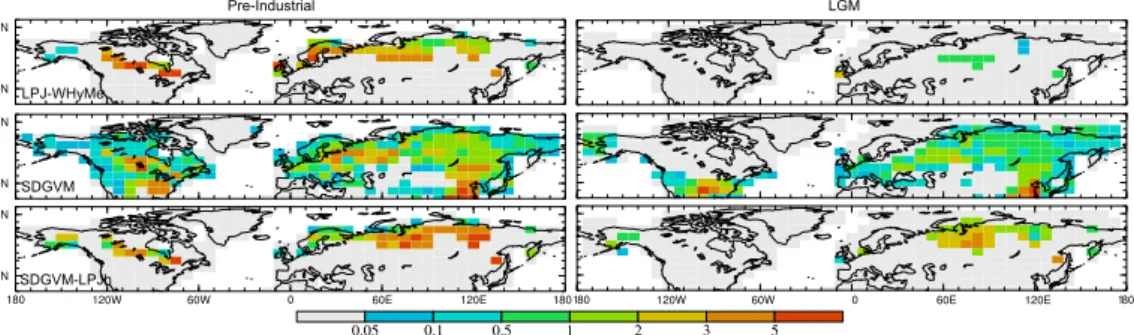
3.3 Transient CH4emissions in LPJ-WHyMe
The peatland emissions respond relatively strongly to the transient changes in climate induced by the freshwater perturbation. The transient decadally averaged CH4 emis-20
sions in LPJ-WHyMe are shown together in Fig. 6. The marked response is especially evident in the 14 kyr simulation, where although the fractional increase in emissions is only 36 % during the warm (GI) phase relative to the unforced (EQ) initial stage, the absolute change is 4 Tg, larger than the increases during the other time periods which are 1.6 and 1.0 Tg yr−1in the LGM and 38 kyr simulations respectively. The magnitude
25
of the transition from GI-HS, i.e. the largest change in each simulation ranges from is 2.8 to 7.5 Tg CH4yr
−1
pat-CPD
9, 3519–3561, 2013D-O Boreal CH4
emissions
P. O. Hopcroft et al.
Title Page
Abstract Introduction
Conclusions References
Tables Figures
◭ ◮
◭ ◮
Back Close
Full Screen / Esc
Printer-friendly Version
Interactive Discussion
Discussion
P
a
per
|
D
iscussion
P
a
per
|
Discussion
P
a
per
|
Discuss
ion
P
a
per
|
tern of GI-HS emission anomalies is shown for these two simulations in Figs. 7 and 8. The largest anomalies are seen over Europe, with the magnitude of change decreasing with latitude. The GI-HS change in the 14 kyr simulation shows a similar feature but a larger area of significant emissions anomalies.
Removing the peat area in Siberia (as shown in Fig. 4) reduces the EQ emission
5
rates by more than 50 % in each time period. Consequently the abrupt reponse (GI-HS) is also reduced, but by less than 50 %. Prescribing extra areas of peat near the North Atlantic in Europe and North America results in a significant increase in emissions. In the 14 kyr simulation, the EQ emissions increases from 11.1 to 21.1 Tg CH4yr
−1
and in the 38 kyr simulation from 4.9 to 14.4 Tg CH4yr
−1
. Similarly the GI-HS response is
10
larger, giving abrupt changes that range from 7.7 to 9.4 Tg CH4yr−1in the 60 and 38 kyr simulations respectively.
4 Analysis
4.1 Comparison with the ice-core inferences
The two earlier studies of Fischer et al. (2008) and Bock et al. (2010) estimated
15
changes in Boreal sources during the deglaciation and D-O events 7 and 8 using a multi-box model and the ice-core interpolar gradient and measured changes in theδD
of CH4. The box model of Bock et al. (2010) requires an increase in the Boreal source
from 6 to 30 Tg CH4yr −1
during the initial rapid phase of the D-O event 8 (their SOM Table 2). For the larger change in atmospheric CH4(increase of 160 ppbv) during the
20
Bølling-Allerød (14kyr) the Boreal source is inferred by Fischer et al. (2008) (see their SOM) to have increased to approximately 36 Tg CH4yr
−1
. The more recent interpolar gradient data from Baumgartner et al. (2012) (from NGRIP and EDML) and prior work of Brook et al. (2000) based on GISP2 and Taylor Dome ice-cores, both suggest more modest increases at high latitudes, with a more important contribution from sub-tropical
25
CPD
9, 3519–3561, 2013D-O Boreal CH4
emissions
P. O. Hopcroft et al.
Title Page
Abstract Introduction
Conclusions References
Tables Figures
◭ ◮
◭ ◮
Back Close
Full Screen / Esc
Printer-friendly Version
Interactive Discussion
Discussion
P
a
per
|
D
iscussion
P
a
per
|
Discussion
P
a
per
|
Discuss
ion
P
a
per
|
Comparing the LPJ-WHyMe changes in CH4emissions across all of the simulations summarised in Table 3 it is clear that none of the simulated changes are near to the values required by the ice-core constraints of Bock et al. (2010). The largest signal occurs in the 38 kyr simulation when the extra NA+EU peat areas are prescribed, and yet this increase is only 40 % of the value required. The change for the equivalent
5
LGM simulation is 8.4 Tg, and is similarly large because although the temperatures are lower, some of the land areas submerged at 38 kyr, are fully exposed at the LGM, increasing the areas of peatland in Europe and eastern North America.
If peatlands can indeed expand rapidly (as suggested by MacDonald et al., 2006), then changes in the emitting area may be an important consideration for the CH4
bud-10
get during D-O events. Assuming the same climate sensitivity of an expanding peat area as that already included in the model, for the 38 kyr (no Sib+EU+NA) simula-tion the extra peatland area required during the abrupt warming would amount to more than a doubling (×2.2). Thus even for the simulation with the highest climate sensitivity
(namely additional peatland is prescribed in the North Atlantic region) the change in
15
total peatland area required to satisfy the conclusions of Bock et al. (2010) appears large when considering the timescale of CH4change which is of the order of 25–100 yr (Huber et al., 2006). This highlights the low magnitude of simulated CH4emission
in-creases in comparison with the overall measured changes in atmospheric CH4 during
these abrupt events.
20
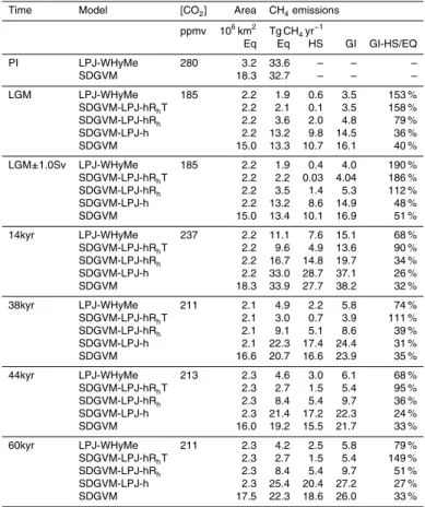
4.2 Comparison with SDGVM
Comparisons are now made between the results from the peatland model LPJ-WHyMe and a wetland model in SDGVM. This should give information on processes important for abrupt CH4 change and provide some insight into the uncertainty associated with the simulated CH4fluxes. The summary values for all of the simulations are shown for 25
emis-CPD
9, 3519–3561, 2013D-O Boreal CH4
emissions
P. O. Hopcroft et al.
Title Page
Abstract Introduction
Conclusions References
Tables Figures
◭ ◮
◭ ◮
Back Close
Full Screen / Esc
Printer-friendly Version
Interactive Discussion
Discussion
P
a
per
|
D
iscussion
P
a
per
|
Discussion
P
a
per
|
Discuss
ion
P
a
per
|
sions at the LGM are 94 and 65 % in LPJ-WHyMe and SDGVM respectively, showing that LPJ-WHyMe is much more sensitive to the LGM low CO2and climate conditions.
The influence of the lowered atmospheric CO2 versus the LGM climate can be
as-sessed by running both models forced with LGM climatology, but pre-industrial CO2 levels. Doing so demonstrates that 88 % of the LGM reduction in emissions is due to
5
climate, with only the 12 % as a result of the prescribed reduction in atmospheric CO2
concentration.
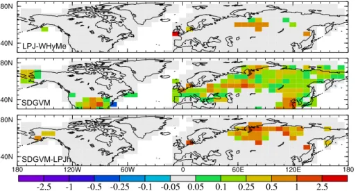
The GI-HS transition for the LGM is 5.4 Tg CH4yr −1
in SDGVM and the spatial pat-tern of GI-HS is shown in comparison with LPJ-WHyMe in Fig. 7. In SDGVM for the Boreal region, the wetland area decreases during the cooling (HS) and increases
dur-10
ing the warming (GI), but the fractional changes are small, and the majority of the change in emissions is a consequence of climatic influence on emission rates rather than changes in the simulated wetland area.
LPJ-WHyMe appears to be more sensitive to the imposed climate, since the propor-tional changes are larger. For example, in the LGM simulations the GI-HS change is
15
153 % of the control LGM value, compared to only 40 % in SDGVM. This may be be-cause the spatial distribution of wetlands is different, or due to other internal processes in the model. We explored this aspect more robustly by configuring a modified version of SDGVM, here denoted SDGVM-LPJ-h, only for peatland grid-cells prescribed in LPJ-WHyMe (in the default configuration). Three other modifications were introduced
20
to SDGVM-LPJ-h in order to minimise differences between the two models: (i) the water-table depth values calculated by LPJ-WHyMe were used instead of those calcu-lated using the SDGVM soil moisture content, (ii) theQ10 of CH4production sensitivity
to temperature was increased from 1.5 to 2.0 and (iii) the orographic correction applied in SDGVM to modify the wetland area and flux was removed. The output of this model
25
SDGVM-LPJ-CPD
9, 3519–3561, 2013D-O Boreal CH4
emissions
P. O. Hopcroft et al.
Title Page
Abstract Introduction
Conclusions References
Tables Figures
◭ ◮
◭ ◮
Back Close
Full Screen / Esc
Printer-friendly Version
Interactive Discussion
Discussion
P
a
per
|
D
iscussion
P
a
per
|
Discussion
P
a
per
|
Discuss
ion
P
a
per
|
h are scaled to match those of LPJ-WHyMe so that differences between the models are more easily quantified.
The emissions in each simulation are compared in Table 4. The LGM drop in SDGVM-LPJ-h is only 60 % compared with 95 % in LPJ-WHyMe showing that the latter remains more sensitive to the imposed climate anomalies. Further the GI-HS
fluctua-5
tion in LPJ-WHyMe is still relatively larger than in SDGVM-LPJ-h at 147 % compared with only 36 % in SDGVM-LPJ-h which is actually lower than the value in SDGVM alone (40 %). This is the result of the different areal extension of wetlands used in the original and hybrid SDGVM versions, specifically the contributions of the larger area of circum-Atlantic wetlands (where the climate anomalies are larger) in the original model
10
version.
In order to further understand these differences the net primary productivity (NPP) averaged over the prescribed peatland gridpoints were compared. Whilst both models show a similar PI value of around 2.5 GtC yr−1, SDGVM shows a much smaller change in NPP at the LGM, with a reduction of around 50 % compared to 90 % in LPJ-WHyMe.
15
This could be a result of the inclusion of the nitrogen cycle in SDGVM or due to dif-ferences in the sensitivities of the plant functional types in the two models. This low sensitivity is not evident in transient anomaly time-series for the abrupt climate events, for which the absolute changes in NPP in the two models are very similar at around
±0.2 GtC yr−1 for the HS and GI phases. The relatively large reduction in NPP
simu-20
lated by LPJ-WHyMe is much greater especially in the colder climates such as the LGM and 38 kyr than in SDGVM. This is because the initial EQ values are lower than in the corresponding SDGVM simulation. Using NPP to predict CH4emissions in the different time periods as a linear function of the ratio of NPP (Whiting and Chanton, 1993) in that time period relative to the pre-industrial, we find that this over-predicts emissions in
25
LPJ-WHyMe by up to 89 % but the maximum error is only±15 % for SDGVM. This
CPD
9, 3519–3561, 2013D-O Boreal CH4
emissions
P. O. Hopcroft et al.
Title Page
Abstract Introduction
Conclusions References
Tables Figures
◭ ◮
◭ ◮
Back Close
Full Screen / Esc
Printer-friendly Version
Interactive Discussion
Discussion
P
a
per
|
D
iscussion
P
a
per
|
Discussion
P
a
per
|
Discuss
ion
P
a
per
|
Taking the same approach for the abrupt transition from HS to GI is less informative as the different carbon stocks, respiration rates and NPP are unlikely to be in equilib-rium during the abrupt climate changes. Instead, a further model hybrid is tested in which the SDGVM-LPJ-h now reads the monthly heterotrophic soil respirationHr from
LPJ-WHyMe . This version is called SDGVM-LPJ-hRh. SDGVM-LPJ-hRhincludes both 5
the soil moisture and water table depth and the carbon substrate from LPJ-WHyMe , but still lacks a representation of the processes related to CH4 transport and oxidation through the soil column, or any direct influence due to the position of the active layer depth.
Again emissions are compared for this model version with the previous 3 models in
10
Table 4. This model shows emissions much closer to those of LPJ-WHyMe. In particular the reduction in emissions at the LGM relative to the pre-industrial is now 89 % which compares favourably with 94 % in LPJ-WHyMe, and is much larger than the value of only 61 % in SDGVM-LPJ-h. This also supports the scaling of NPP to calculate the EQ emission rates in different time periods. However, this model version
(SDGVM-LPJ-15
hRh) still considerably underestimates the transient emission changes seen in
LPJ-WHyMe. For example in the LGM simulation the increase during the GI relative to the EQ is 84 % in LPJ-WHyMe, but only 33 % in SDGVM-LPJ-hRh, though this is far larger
than the 10 % in SDGVM-LPJ-h. The values for the warmest simulation (14 kyr) follow a similar pattern: 36 % for LPJ-WHyMe versus 18 % in SDGVM-LPJ-hRh and 12 % in
20
SDGVM-LPJ-h. Thus whilst the long-term equilibrium (EQ) values can be reconciled by taking the carbon substrate from LPJ-WHyMe in this hybrid model setup, the transient sensitivity of LPJ-WHyMe cannot.
A final model version SDGVM-LPJ-hRhT now takes the 25cm soil temperature
pre-dicted by LPJ-WHyMe in the SDGVM-LPJ-hRhmodel rather than using the surface air 25
temperature simulated by FAMOUS. The 25cm soil temperature is chosen because it controls the rates of heterotrophic respiration within LPJ-WHyMe for CH4 emissions
(Wania et al., 2010). The LGM reduction in emissions in SDGVM-LPJ-hRhT is 94 %,
CPD
9, 3519–3561, 2013D-O Boreal CH4
emissions
P. O. Hopcroft et al.
Title Page
Abstract Introduction
Conclusions References
Tables Figures
◭ ◮
◭ ◮
Back Close
Full Screen / Esc
Printer-friendly Version
Interactive Discussion
Discussion
P
a
per
|
D
iscussion
P
a
per
|
Discussion
P
a
per
|
Discuss
ion
P
a
per
|
same in SDGVM-LPJ-hRhT and LPJ-WHyMe (as shown in Table 4). This suggests that the effects of soil freezing and the position of the active layer depth increase the sensitivity of the CH4 emissions in cold regions and that only by including this can we
reconcile the magnitude of change in CH4 emissions seen in LPJ-WHyMe with the hybrid model considered here. Other differences remain, particularly in the remaining
5
time periods and these must be related to other differences between LPJ-WHyMe and SDGVM not considered in the above analysis.
4.3 Concentration predictions
The modelled changes in emissions between the cold and warm states (HS and GI) are now used to calculate the likely change in atmospheric CH4. This allows direct 10
comparison with the ice-core record for all events simulated without the complications arising from deconvolving the emissions estimates from the interpolar gradient. Numer-ical simulations of the major influences on the atmospheric CH4lifetime during a glacial
abrupt warming event suggest that the lifetime may be relatively constant (Levine et al., 2012). Thus we employed a constant lifetime of 8.6 yr (following prior work: Hopcroft
15
et al., 2011) and assumed a uniform conversion of emissions to atmospheric concen-tration of 2.75 ppbv Tg−1. The results are increased by 10 % to account for the self feedback of CH4 on its own lifetime, based on analysis of glacial atmospheric chem-istry simulations (Levine et al., 2011). The SDGVM total pre-industrial emissions are scaled to match the value of 147 Tg CH4yr
−1
used by Valdes et al. (2005) and Levine
20
et al. (2011) in order to be more consistent with previous calculations of atmospheric concentration changes for glacial time periods. This means that the total concentra-tion predicconcentra-tions are slightly smaller than those predicted in previous work (Hopcroft et al., 2011). The LPJ-WHyMe values are given as differences with the emissions from SDGVM over the equivalent area, to illustrate the effect of the inclusion of more
com-25
CPD
9, 3519–3561, 2013D-O Boreal CH4
emissions
P. O. Hopcroft et al.
Title Page
Abstract Introduction
Conclusions References
Tables Figures
◭ ◮
◭ ◮
Back Close
Full Screen / Esc
Printer-friendly Version
Interactive Discussion
Discussion
P
a
per
|
D
iscussion
P
a
per
|
Discussion
P
a
per
|
Discuss
ion
P
a
per
|
below 45◦N which do not contain prescribed peatlands in the equivalent LPJ-WHyMe scenario.
The maximum calculated change in atmospheric CH4 calculated by summing
SDGVM (<45◦N) and LPJ-WHyMe (≥45◦N) is 102 ppbv in the 14 kyr case, whilst the
maximum total change is only 86 and 95 ppbv in the 60 and 44 kyr cases respectively.
5
Depending on the area of peat prescribed, the LPJ-WHyMe model can simulate both less and more change than in SDGVM, with the exception of the 14kyr case. The predicted CH4 changes are compared against ice-core data in Table 1. The SDGVM
results underestimate the events by between 23–57 %. Inclusion of LPJ-WHyMe only improves the agreement with ice-core data when the maximum peat area simulations
10
are used in the LGM, 44 and 60 kyr simulations. In these simulations LPJ-WHyMe in-creases the change by up to 10 %. Despite the increased transient sensitivity of the LPJ-WHyMe model, the results still suggest underestimation of the observed rapid CH4 increases. This is partly because LPJ-WHyMe predicts lower initial (EQ)
emis-sions than SDGVM during each time period.
15
The significant variation in the amplitude of the abrupt CH4changes as evident from the ice-core data (Flückiger et al., 2004; Huber et al., 2006) does not appear to be well replicated in the simulations. For example, the CH4 change at D-O event 17 is 65 %
larger than for event 11. Singarayer et al. (2011) demonstrated that the SDGVM model is able to replicate the orbital timescale changes in CH4emissions rather well. Hence 20
the lack of variability in the size of the abrupt changes simulated here could result from some feature of the physical climatic forcing. For example, the abrupt changes in the AMOC are very similar in the different time periods considered.
5 Discussion
We have performed a series of transient coupled GCM simulations of five time periods
25
CPD
9, 3519–3561, 2013D-O Boreal CH4
emissions
P. O. Hopcroft et al.
Title Page
Abstract Introduction
Conclusions References
Tables Figures
◭ ◮
◭ ◮
Back Close
Full Screen / Esc
Printer-friendly Version
Interactive Discussion
Discussion
P
a
per
|
D
iscussion
P
a
per
|
Discussion
P
a
per
|
Discuss
ion
P
a
per
|
North Atlantic region, mostly as a result of increased heat transport from the resurgent AMOC, but also partly deriving from feedbacks from sea-ice cover and atmospheric heat transport. The warming over Greenland in the model is of the order of 8–9◦C which is at the lower end of the ice-core reconstructions. Doubling, the magnitude of the freshwater forcing (which equates to 10 m/century sea-level rise) does not
repro-5
duce the largest magnitude of warming observed in Greenland of up to 16◦C (Huber et al., 2006; Wolffet al., 2010).
The inferred source changes for northern sources from recent data of Baumgartner et al. (2012) (in agreement with inferences of Brook et al. (2000)) suggest that northern sources were approximately halved during the last glacial period. The strong reduction
10
in northern peatland emissions in LPJ-WHyMe is consistent with this inference, but it is not possible to differentiate between the boreal and sub-tropical northern sources using the ice-core interpolar gradient and so quantitative comparison between LPJ-WHyMe and the ice-core-based inference is difficult.
Using the transient monthly-mean GCM outputs, we have forced a series of
sim-15
ulations of the LPJ-WHyMe peatland and CH4 emissions models. Comparisons with
inferences drawn from the ice-core derived inter-hemispheric gradient and δDCH4 of
CH4 Bock et al. (2010) indicate that the model simulations significantly under-predict
the abrupt changes in emissions, but this is in agreement with the newer lower values for the glacial and interstadial interpolar gradient (Baumgartner et al., 2012). Simple
20
calculations of the atmospheric concentration changes in response to global emission increases also under-predict the measured changes from ice-cores.
Comparison of the results with an independent DGVM (SDGVM) suggests that the model complexity of LPJ-WHyMe leads to increased sensitivity, although there are major structural differences between the models analysed which hinders quantitative
25
CPD
9, 3519–3561, 2013D-O Boreal CH4
emissions
P. O. Hopcroft et al.
Title Page
Abstract Introduction
Conclusions References
Tables Figures
◭ ◮
◭ ◮
Back Close
Full Screen / Esc
Printer-friendly Version
Interactive Discussion
Discussion
P
a
per
|
D
iscussion
P
a
per
|
Discussion
P
a
per
|
Discuss
ion
P
a
per
|
more sensitive than the SDGVM-LPJ-h model and up to 4 times more sensitive than the SDGVM-LPJ-hRhmodel. This analysis indicated that the carbon substrate in
LPJ-WHyMe is more sensitive to the imposed climate, most likely due to the influence of soil freezing on plant moisture availability, whilst hydrological differences between LPJ-WHyMe and SDGVM were less important. Inclusion of the influence of soil freezing on
5
the carbon substrate supply (by taking heterotrophic respiration from LPJ-WHyMe in the SDGVM-LPJ-hRh model) was mostly able to reproduce the base (EQ) emissions in different time periods. However, it appears that the inclusion of vertically resolved emission, transport and oxidation of CH4, and their dependence on the active layer
depth is crucial for fully resolving the magnitude of the transient changes in emissions
10
in these simulations.
A weak CH4 response to abrupt AMOC variations has also been found in prior
work using SDGVM and ORCHIDEE models forced with FAMOUS climate output (Hopcroft et al., 2011; Ringeval et al., 2013), and in a newer version of LPJ-WHyMe forced with a freshwater scenario under modern climatic conditions using a different
15
model, CCSM1.4 (Zürcher et al., 2013). A recent model intercomparison (Melton et al., 2013) quantified the sensitivities of 10 CH4emissions models including LPJ-WHyMe, SDGVM and ORCHIDEE. This showed that current models span a range of sensitiv-ities to temperature, precipitation and atmospheric CO2. Examining the extra-tropical
response to a uniform temperature and precipitation increase of 3.4◦C and 3.9 %
re-20
specitively, these three models span the range from−26 to+24 % change in response to warming (ORCHIDEE and LPJ-WHyMe respectively) and from 3 to 10 % change in response to precipitation increase (SDGVM and ORCHIDEE respectively). Together this suggests that the main conclusions reached here may be robust, but that inter-model differences are still large and require further investigation.
25
CPD
9, 3519–3561, 2013D-O Boreal CH4
emissions
P. O. Hopcroft et al.
Title Page
Abstract Introduction
Conclusions References
Tables Figures
◭ ◮
◭ ◮
Back Close
Full Screen / Esc
Printer-friendly Version
Interactive Discussion
Discussion
P
a
per
|
D
iscussion
P
a
per
|
Discussion
P
a
per
|
Discuss
ion
P
a
per
|
vegetation. Two recent studies with 3-D atmospheric chemistry-transport simulations suggested that the combined impact of these two effects leads to a negligible change in CH4lifetime both for the G-IG transition and for abrupt climate events (Levine et al.,
2011, 2012).
Other potentially relevant CH4sources not addressed in this work include biomass
5
burning, thaw lakes and the oceans. Whilst records of charcoal suggest a dynamic re-lationship between climate and biomass burning (Daniau et al., 2010), ice-core isotopic evidence appears to argue against substantial contributions on either the glacial-inter glacial (Fischer et al., 2008) or abrupt time-scales (Bock et al., 2010). Thaw lakes are a large source of uncertainty as they are difficult to represent realistically in global-scale
10
models. Controversy remains over whether geological evidence signifies a rapid ex-pansion of thaw lakes during the abrupt CH4increase at the end of the Younger-Dryas (Walter et al., 2007; Reyes and Cooke, 2011) and further work is required to establish the magnitude and sensitivity of thaw lake emissions under atmospheric warming sce-narios. Evidence for methanogenic bacterial communities in sub-glacial environments
15
suggests a sub-glacial source of CH4 (Wadham et al., 2008). The potential influence
of subglacial environments on atmospheric CH4 or on carbon substrate supply
subse-quent to deglaciation is uncertain.
A primary limitation in the current study is the prescription of peatland areas within the LPJ-WHyMe model. We have attempted to address this uncertainty by analysing
20
the signals from 4 different distributions for each time period, but stronger palaeo-time constraints on peatland areas would be invaluable. Another approach could rely on reconstructions of ice-sheet areas through time, adding peat areas as a function of time since deglaciation. Information on the area of glaciation for times prior to the Last Glacial Maximum is very limited due to the destruction of landscape markers by the
ex-25
CPD
9, 3519–3561, 2013D-O Boreal CH4
emissions
P. O. Hopcroft et al.
Title Page
Abstract Introduction
Conclusions References
Tables Figures
◭ ◮
◭ ◮
Back Close
Full Screen / Esc
Printer-friendly Version
Interactive Discussion
Discussion
P
a
per
|
D
iscussion
P
a
per
|
Discussion
P
a
per
|
Discuss
ion
P
a
per
|
6 Conclusions
Results from these simulations with a coupled atmosphere-ocean GCM and two ecosystem CH4 emissions models (SDGVM and LPJ-WHyMe) suggest that changes
in the Atlantic MOC are unable to fully explain abrupt changes in atmospheric CH4 as reconstructed from ice-cores. The weak peatland source changes are consistent
5
with new interpolar gradient but the total emissions increases underestimate the mea-sured changes in atmospheric concentration. Relative to a more generalized wetland scheme (such as SDGVM), the inclusion of peatland and permafrost processes in the LPJ-WHyMe model increases the climatic sensitivity of CH4emissions. This increased
sensitivity in the peatland model under equilibrium conditions is mostly due to diff
er-10
ences in the carbon cycle productivity, whilst the increased sensitivity to abrupt warm-ing is also partly due to the effects of freezing on soil thermodynamics. The higher sensitivity in LPJ-WHyMe however implies low simulated baseline emissions in each of the glacial time periods. This means that the rapid changes in CH4 emissions are
of similar magnitude in the peatland model as in the generalized wetland scheme. The
15
variability in the magnitude of the abrupt CH4rises inferred from the ice-core record is also not convincingly replicated in the model, and this could be related to some feature of the climate scenarios used.
The CH4changes during D-O events are extremely large when compared with natu-ral contemporary variations, and thus constitute important targets for improved
under-20
standing of the global CH4 cycle. Changes in wetland emissions during these events
have been inferred to be relatively strong and modelling efforts should focus on how different weltand process representations (Ringeval et al., 2013) and mechanisms of climate change might be important for understanding D-O events. Recent studies have highlighted potential alternative mechanisms for abrupt warming aside from changes
25
CPD
9, 3519–3561, 2013D-O Boreal CH4
emissions
P. O. Hopcroft et al.
Title Page
Abstract Introduction
Conclusions References
Tables Figures
◭ ◮
◭ ◮
Back Close
Full Screen / Esc
Printer-friendly Version
Interactive Discussion
Discussion
P
a
per
|
D
iscussion
P
a
per
|
Discussion
P
a
per
|
Discuss
ion
P
a
per
|
diversify beyond freshwater the range of perturbations imposed on coupled GCMs in this context, particularly as this could lead to different patterns of climate change and hence CH4emissions.
Acknowledgements. This work was funded by the joint UK and France QUEST-INSU DESIRE (Dynamics of the Earth System and the Ice-core Record) project, and partly by a NERC UK
5
grant Earth System Modelling of Abrupt Climate Change. We thank James Levine, Bruno Ringeval and Eric Wolff for discussions on many aspects of the CH4 cycle and abrupt cli-mate change. This work was carried out using the computational facilities of the Advanced Computing Research Centre, University of Bristol – http://www.bris.ac.uk/acrc/.
References
10
Baumgartner, M., Schilt, A., Eicher, O., Schmitt, J., Schwander, J., Spahni, R., Fischer, H., and Stocker, T. F.: High-resolution interpolar difference of atmospheric methane around the Last Glacial Maximum, Biogeosciences, 9, 3961–3977, doi:10.5194/bg-9-3961-2012, 2012. 3521, 3531, 3532, 3539
Beerling, D. J. and Woodward, F. I.: Vegetation and the Terrestrial Carbon Cycle: Modelling the
15
first 400 Million Years, Cambridge: Cambridge University Press, 2001. 3522, 3526
Berger, A. and Loutre, M.: Insolation values for the climate of the last 10 million years, Quater-nary Sci. Rev., 10, 297–317, 1991. 3523
Blunier, T. and Brook, E.: Timing of Millennial-Scale Climate Change in Antarctica and Green-land During the Last Glacial Period, Science, 291, 109–112, 2001. 3550
20
Bock, M., Schmitt, J., Moller, L., Spahni, R., Blunier, T., and Fischer, H.: Hydrogen Isotopes Pre-clude Marine Hydrate CH4Emissions at the Onset of Dansgaard-Oeschger Events, Science, 328, 1686–1689, 2010. 3531, 3532, 3533, 3539, 3541
Brook, E. J., Harder, S., Severinghaus, J., Steig, E. J., and Sucher, C. M.: On the origin and timing of rapid changes in atmospheric methane during the last glacial period, Global
Bio-25
geochem. Cy., 14, 559–572, 2000. 3521, 3532, 3539
CPD
9, 3519–3561, 2013D-O Boreal CH4
emissions
P. O. Hopcroft et al.
Title Page
Abstract Introduction
Conclusions References
Tables Figures
◭ ◮
◭ ◮
Back Close
Full Screen / Esc
Printer-friendly Version
Interactive Discussion
Discussion
P
a
per
|
D
iscussion
P
a
per
|
Discussion
P
a
per
|
Discuss
ion
P
a
per
|
Chen, Y.-H. and Prinn, R.: Estimation of atmospheric methane emissions between 1996 and 2001 using a three-dimensional global chemical transport model, J. Geophys. Res., 111, D10307, doi:10.1029/2005JD006058, 2006. 3530, 3552
Clement, A. and Peterson, L.: Mechanisms of Abrupt Climate Change of the Last Glacial Period, Rev. Geophys., 46, RG4002, doi:10.1029/2006RG000204, 2008. 3521, 3542
5
Dällenbach, A., Blunier, T., Flückiger, J., Stauffer, B., Chappellaz, J., and Raynaud, D.: Changes in the atmospheric CH4gradient between Greenland and Antarctica during the Last Glacial and the transition to the Holocene, Geophys. Res. Lett., 27, 1005–1008, 2000. 3521 Daniau, A.-L., Harrison, S., and Bartlein, P.: Fire regimes during the Last Glacial, Quaternary
Sci. Rev., 29, 2918–2930, 2010. 3541
10
Elliot, M., Labeyrie, L., and Duplessy, J.-C.: Changes in North Atlantic deep-water formation associated with the Dansgaard-Oeschger temperature oscillations (60–10 ka), Quaternary Sci. Rev., 21, 1153–1165, doi:10.1016/S0277-3791(01)00137-8, 2002. 3530
Fischer, H., Behrens, M., Bock, M., Richter, U., Schmitt, J., Loulergue, L., Chappellaz, J., Spahni, R., Blunier, T., Leuenberger, M., and Stocker, T. F.: Changing boreal methane
15
sources and constant biomass burning during the last termination, Nature, 452, 864–867, 2008. 3531, 3532, 3541
Flückiger, J., Blunier, T., Stauffer, B., Chappellaz, J., Spahni, R., Kawamura, K., Schwan-der, J., Stocker, T. F., and Dahl-Jensen, D.: N2O and CH4 variations during the last glacial epoch: Insight into global processes, Global Biogeochem. Cy., 18, GB1020,
20
doi:10.1029/2003GB002122, 2004. 3521, 3522, 3538, 3550
Frolking, S., Roulet, N. T., Tuittila, E., Bubier, J. L., Quillet, A., Talbot, J., and Richard, P. J. H.: A new model of Holocene peatland net primary production, decomposition, water balance, and peat accumulation, Earth Syst. Dynam., 1, 1–21, doi:10.5194/esd-1-1-2010, 2010. 3541 Ganopolski, A. and Rahmstorf, S.: Rapid changes of glacial climate simulated in a coupled
25
climate model, Nature, 409, 153–155, 2001. 3521, 3524
Gerten, D., Schaphoff, S., Haberlandt, U., Lucht, W., and Sitch, S.: Terrestrial vegetation and water balance: Hydrological evaluation of a dynamic global vegetation model, J. Hydrology, 286, 249–270, 2004. 3523
Gherardi, J.-M., Labeyrie, L., McManus, J. F., Francois, R., Skinner, L. C., and Cortijo, E.:
Evi-30
CPD
9, 3519–3561, 2013D-O Boreal CH4
emissions
P. O. Hopcroft et al.
Title Page
Abstract Introduction
Conclusions References
Tables Figures
◭ ◮
◭ ◮
Back Close
Full Screen / Esc
Printer-friendly Version
Interactive Discussion
Discussion
P
a
per
|
D
iscussion
P
a
per
|
Discussion
P
a
per
|
Discuss
ion
P
a
per
|
Gordon, C., Cooper, C., Senior, C. A., Banks, H., Gregory, J. M., Johns, T. C., Mitchell, J. F. B., and Wood, R. A.: The simulation of sst, sea ice extents and ocean heat transports in a version of the Hadley Centre coupled model without flux adjustments, Clim. Dynam., 16, 147–168, 2000. 3523
Granberg, G., Grip, H., Ottosson Löfvenius, M., Sundh, I., Svensson, B. H., and Nilsson, M.: A
5
simple model for simulation of water content, soil frost, and soil temperatures in boreal mixed mires, Water Resour. Res., 35, 3771–3782, 1999. 3551
Halsey, L., D. Vitt, and Gignac, L.: phSphagnum-dominated Peatlands in North America Since the Last Glacial Maximum: Their Occurrence and Extent, The Bryologist, 103, 334–352, 2000. 3526
10
Harrison, S. and Sanchez-Goñi, M.: Global patterns of vegetation response to millennial-scale variability and rapid climate change during the last glacial period, Quaternary Sci. Rev., 29, 21–22, 2957–2980, 2010. 3529, 3530
Hendy, I. and Kennett, J.: Dansgaard-Oeschger cycles and the California Current System: Planktonic foraminiferal response to rapid climate change in Santa Barbara Basin, Ocean
15
Drilling Program hole 893A, Paleoceanography, 15, 30-42, 2000. 3520, 3530
Hopcroft, P., Valdes, P., and Beerling, D.: Simulating idealized Dansgaard-Oeschger events and their potential impacts on the global methane cycle, Quaternary Sci. Rev., 30, 3258–3268, 2011. 3522, 3524, 3529, 3537, 3540, 3550, 3553
Huber, C., Leuenberger, M., Spahni, R., Flückiger, J., Schwander, J., Stocker, T., Johnsen, S.,
20
Landais, A., and Jouzel, J.: Isotope calibrated Greenland temperature record over Marine Isotope Stage 3 and its relation to CH4, Earth Planetary Sci. Letts., 243, 504–519, 2006. 3520, 3521, 3533, 3538, 3539, 3550
Kanner, L. C., Burns, S. J., Cheng, H., and Edwards, R. L.: High-Latitude Forcing of the South American Summer Monsoon During the Last Glacial, Science, 335, 570–573, 2012. 3520,
25
3529
Kleinen, T., Brovkin, V., and Schuldt, R. J.: A dynamic model of wetland extent and peat accu-mulation: results for the Holocene, Biogeosciences, 9, 235–248, doi:10.5194/bg-9-235-2012, 2012. 3541
Korhola, A., Ruppel, M., Seppä, H., Väliranta, M., Virtanen, T., and Weckström, J.: The
im-30