Bankruptcy forecasting models civil construction

BANKRUPTCY FORECASTING MODELS

CIVIL CONSTRUCTION

Ana Filipa Roussado Silva

Project submitted as requirement for the conferral of

Master in Finance

Leader:

Prof. Doctor José Joaquim Dias Curto, Prof. Auxiliary, ISCTE Business School, Quantitative Methods Department

Co advisor:

Prof. Doctor Emanuel Freire Torres Gamelas, Prof. Auxiliary, ISCTE Business School, Accounting Department

2

Acknowledgment

First, I want to thank my parents for all the support that they gave me all these years. Without them I couldn't have completed this stage of my life! They are my lifeline and this thesis is my way to I can say THANK YOU for all that you have done for me!

Secondly, I would like to thank my brother Fernando, who encouraged me to do this project. Sometimes I feel that in some way and especially in his own way he is an example for me.

Thirdly, I would like to acknowledge my leader professor Dias Curto and co-leader professor Emanuel Gamelas for all patience, dedication, availability and support they offered whenever I needed.

Finally I would like to thank all people that directly and indirectly made me feel focused: my family and my friends that encouraged me and believed that I could do this; without Nena this project would have been more complicated; and GesARRENDA, especially Rita and Nuno, thank you for all the support and time that I needed to complete this dissertation.

3

Resumo

O termo insolvência é uma das palavras mais ouvidas hoje em dia quando falamos da actual crise económica. Consiste na impossibilidade da empresa fazer face aos seus compromissos perante os seus credores, isto é, a impossibilidade de liquidar as suas dívidas.

O risco de falência pode estar relacionado com factores internos e externos à empresa (qualidade de gestão, concorrência, capacidade de financiamento).

Segundo dados existentes, em 1932 Fitzpatrick foi o primeiro a estudar este tema, e desde essa época, vários teóricos aperfeiçoaram os modelos de previsão já existentes. Recorrendo a dados contabilísticos foram criados métodos para prever estas situações, é o caso do modelo LOGIT, um modelo análise logística.

Este estudo tem como objectivo aferir qual a probabilidade de uma empresa entrar em situação de insolvência com base nas empresas solventes no mesmo sector (construção civil), durante o período de 2000 a 2012. Para tal, vai utilizar-se uma amostra de empresas falidas e não falidas e um conjunto de rácios económico-financeiros calculados através dos balanços e demonstração de resultados das empresas em análise. Esta análise financeira calculada por meio dos índices surge da necessidade de avaliar o quão saudável a empresa está financeiramente, auxiliando os investidores, credores e administradores na predição de situações favoráveis ou dificuldades económicas.

Vão ser utilizados oito rácios, dois quais, apenas quatro (ROE, ROA, Profit Margin e Coverage Index) se mostraram estatisticamente significativos com base na análise feita pelo modelo LOGIT. O modelo estimado, consegue prever correctamente 92.86% dos casos de solvência/insolvência.

Palavras-chave: Previsão de insolvência, Logit, Indicadores económico-financeiros,

Falência.

JEL Sistema de Classificação: G33 (Falência – Liquidação) e C53 (Estimação e Previsão de

Modelos - Modelos de Simulação)

4

Abstract

Insolvency is one of the most common terms heard today when the current economic crisis is brought up. It can be defined as the inability of the company to deal with the responsibilities they have towards its creditors, in other words, the inability to pay its debts. The risk of bankruptcy can be a result of internal and external factors, such as quality of managements, competitors and financing capacity.

According to data from 1932, Fitzpatrick is the first one to study this topic. Since then, many researchers have made improvements on the forecasting model. Using accounting data methods were created to predict these bankruptcy situations. One of these methods is the Logit model, a model of techniques of logistic analysis.

This study aims to assess the probability of insolvency based on solvent companies in the same sector (construction) during the period 2000 to 2012.

For this, it will use a sample of bankrupt and non-bankrupt firms and a set of economic and financial ratios. These ratios are calculated from the data balance sheets and income statements of the companies under analysis. This financial analysis, which is calculated using the ratios, is necessary to evaluate how healthy the company is financially, therefore assisting investors, creditors and managers when predicting favorable situations or economic difficulties.

Based on the ratios used and looking for the results of the Logit Model, just four ratios remain statistically significant (ROE, ROA, Profit Margin and Coverage Index). The estimated model can predict correctly 92.86% of the cases of solvency / insolvency.

Key words: Failure prediction, Logit, economic and financial indicators, bankruptcy.

JEL Classification System: G33 (Bankruptcy - Liquidation) and C53 (Forecasting and

Prediction Methods - Simulation Methods).

5

Abbreviations

AS: Asset Turnover

CEO: Chief of executive office CI: Coverage Index

CIRE: Código de insolvência e recuperação de empresas DI: Debt Index

D/E: Debt-to-Equity

EBIT: Earnings Before Interest and Taxes FGV: Fundação Getúlio Vargas

FL: Financial Leverage GNP: Gross National Product

IIC: Instituto de Informação ao Consumidor L: Liquidity

LR: Likelihood Ratio M.: Mean

MBA: Master of Business Administration PER: Processo Especial de Revitalização PM: Profit Margin

ROE: Return on Equity ROA: Return on Assets

SPSS: Statistical Package for the Social Sciences VIF: Variance Inflation Factor

6

Index

Index of tables ... vii.

Index of graphs ... vii.

Index of equations ... vii.

1. Introduction ... 8 2. Insolvency in Portugal ... 10 3. Methodology ... 23 3.1 Logit Model ... 23 3.2 Independent variables ... 26 4. Empirical Study ... 30

4.1 Selection of the sample ... 30

4.2 Results of solvent companies ... 33

4.3 Results of insolvent companies ... 35

4.4 Correlation of the sample variables ... 39

5 Estimation of the model ... 41

5.1 The Logit ... 41

5.2 Multicollinearity problems ... 44

6. Conclusions ... 53

7. Bibliography ... 55

8. Annexes ... 60

8.1 Correlation of the sample ... 60

8.2 VIF – Condition Index ... 61 vi.

7

Index of tables

Table 1: Predict Results by James A. Holson ... 18

Table 2: Resume of previously studies ... 22

Table 3: Statistics for solvent companies ... 31

Table 4: Mean solvent companies, liquidity ratios. ... 35

Table 5: Statistics for insolvent companies ... 35

Table 6: Mean insolvent companies, liquidity analysis ... 38

Table 7: Correlations between independent variables ... 39

Table 8 Negative correlations by SPSS ... 40

Table 9: Sample ... 41

Table 10: Classification of the sample ... 41

Table 11: Logit Model, with all independent variables ... 42

Table 12: Expected signal of ratios in a predicting insolvency. ... 43

Table 13: VIF ... 45

Table 14: Logit Model, without mean debt-to-equity ... 46

Table 15: Logit Model, without liquidity and debt-to-equity ... 47

Table 16: Logit Model, without liquidity, asset turnover and debt-to-equity ... 48

Table 17: Logit model, only with statistically significant variables ... 49

Table 18: Prediction evaluation of the model ... 51

Index of graphs

Graph 2: Logit transformation ... 24

Graph 3: Mean of solvent companies, profit margin analysis. ... 33

Graph 4: Mean of solvent companies, asset turnover analysis. ... 34

Graph 5: Mean of solvent companies, ROA analysis. ... 34

Graph 6: Mean insolvent companies, profit margin vs debt index analysis. ... 36

Graph 7: Mean insolvant companies, asset turnover analysis. ... 37

Index of equations

Equation 2: Logistic regression model ... 24

Equation 3: Logistic model ... 42

Equation 4: Logistic regression model with all of the independent variables. ... 43

Equation 5: Logistic model ... 50

Equation 6: Logistic regression model with statistically significant variables ... 50

8

1. Introduction

The topic of this dissertation will focus on forecasting methods of bankruptcy in the construction industry. This theme emerges from the current economic situation of the country. Portugal is in a period of economic crisis that has been worsening day by day over the last few years.

It is possible to identify the main reasons why so many companies become bankrupt. They are: the constraints on access to credit, shrinking margins in the business and delays in payments from the state.

It’s important to find a tool that allows the analysis and monitors the performance of

the activity in a dynamic way in order to alert and anticipate financial crisis. In this context, it is necessary to develop forecasting techniques to anticipate financial or management difficulties as soon as possible to reduce the losses for all people involved in the business: investors, employees, partners and other interested parties.

This is a theory which has been developed over the years. The studies started in 1932 with Fitzpatrick; he was a pioneer in a bankrupt prediction, the values of financial ratios in bankrupt and non-bankrupt firms were compared with each other and it was found that they were poorer for failed firms.

In 1966 the pioneering study of Beaver presented the univariate approach of discriminant analysis. Beaver concludes that the best ratios to describe the bankrupt process are “working capital funds/total assets” and “net income/total assets”, which correctly identified 90% and 88% of the cases.

In 1968 Altman expanded this analysis to multivariate analysis. Altman was one of the first researchers to use multiple discriminant analysis as a tool for predicting insolvencies. For him, the insolvency of a company is declared when the shareholders receive a return on their investments which is lower than the profitability offered by the market for investments of similar risk.

As a result of some disadvantages showed by Altman, Ohlson in 1980 is the first to apply logit analysis on the problem of bankruptcy prediction.

9 Based on some results of Ohlson, it will be estimated the probability of company going to bankruptcy, taking into account the economic and financial ratios, based on the Logit Model.

Logistic regression analysis will be used to investigate the relationship between binary response probability (0: non – bankrupt, 1: bankrupt) and explanatory variables (economic and financial ratios). The advantage of this method is that it does not assume multivariate normality and equal covariance matrices as discriminant analysis does. Logit analysis incorporates non-linear effects, and uses the logistical cumulative function in predicting a bankruptcy.

Thus, this dissertation will start to explain, in the first place, what insolvency is and how it has been developed in Portugal. Secondly, it will be expressed how to deal with this process, this means, what are the phases of the insolvency process. Thirdly, it will approach the authors who studied this topic in the past, and which conclusions they have reached. In fourth place, based on the sample obtained, it will be explained which model will be used to find the conclusions (which model and which variables), and finally, the conclusions will be compared with those reached by other authors.

After reading this dissertation, it will be possible to understand which indicators managers must use to avoid situations of financial failure.

10

2. Insolvency in Portugal

The term insolvency is frequently used to talk about the actual economic crisis. This term means that a particularly company is unable to meet its obligations towards its creditors, ie, the inability to pay its debts. In order to understand if a company is in this type of situation, it is necessary to prepare an analysis of its economic situation. On one hand, a company can be insolvent because it is unable to meet its obligations by lack of access to credit or by illiquidity, but on the other hand, a company can be suffering a particularly financial difficulty that is preventing it from settling its debts on time.

According to paragraph 1 of Article 3 of the “Código da Insolvência e Recuperação

de Empresas” (CIRE), it is considered insolvency when the borrower is unable to pay his

debts. Thus, in the context of a company, this means that the liability exceeds the assets, implying an unsustainable situation, and the inability for the company to pay off its commitments.

Paraphrasing Bruna Saniele, it is important for the small entrepreneurs to have access to a business plan, which enables them to understand if an investment is as interesting as it seems, or to (re) define the purpose of their businesses.

Another important point highlighted by Saniele, is that the entrepreneur needs to have a good knowledge about the market in which he will operate; he needs to understand what the customer demand is in order to identify which products the customer will want to buy. "The initial planning is essential to ensure the firm's survival. The firms that prepare have a chance to survive for the first four years (25%) while one that does not prepare has a one in five chance (only 20%)," says Messias.

Another author mentioned by Saniele is Edison Kalaf, Professor of the Business School of São Paulo, he says that there are five main factors that lead the company into bankruptcy. The first is the lack of market. Most entrepreneurs opening businesses only have technical knowledge; they don’t know how to manage the company, neither how the market where they will operate works.

Another risk factor is that business owners are unaware of the working capital they will need. They tend to save only the necessary amount for the company to survive the first

11 few months of life (income, fixed costs, staff costs), and forget their own personal costs. This means that in the future, they have to resort to the capital of the company to support their debts. Often, this capital withdrawn by the managers is needed afterwards for the maintenance of the company.

Regarding the lack of disclosure, another point that should be taken into account, must be set from the first steps of the company. The marketing is one of the most important costs for the company, because without marketing it cannot attract customers and consequently sales will not increase.

Regarding the financial matters, and according to Kalaf, it is very important to have financial and stock control. It is crucial that the manager is aware of where he can and where he should not invest the company’s money. It is also very important that he is aware of the material he has in stock to avoid unnecessary purchases.

Finally, the last point mentioned by Kalaf is the qualification of employees. Often these have initial training which plays an important role in the presentation of the company. If they are not aware of the image that the company wants to convey they may ultimately hurt the business.

According to Kalaf, these are some of the reasons that may lead the company into bankruptcy. It then becomes important to realize when these signs are evident and will lead the company into insolvency.

Rubens Famá and J. William Grava (2000) identifies several symptoms that may indicate a situation of bankruptcy, such as:

 Reduction of dividends;

 Closure of installations;

 Constant losses;

 Extraordinary layoffs;

 Outgoing CEO;

 Drop in share prices.

It is important to note that the topics mentioned above are just indicators, they do not themselves indicate a bankruptcy situation; the dividend reduction factor, for example, could

12 indicate that a company is finding it difficult to maintain a sustainable cash flow, but could also represent the targeting of capital for an investment opportunity.

It then becomes important to find a tool that allows the analysis and monitors the performance of the activity in a dynamic way in order to alert and anticipate financial crises. In this context, it is necessary to develop forecasting techniques to anticipate financial or management difficulties as soon as possible. This type of instrument provides warning signs for those involved in the business: investors, employees, partners and other interested parties wishing to reduce losses.

There are some stages before the company can be declared insolvent and the bankruptcy process requires some deadlines so that a company can be declared as bankrupt. The first stage consists on the evaluation of the economic situation. Being insolvent means that a company is unable to meet its obligations, but the disability must be certified at one point through the declaration of insolvency. This statement can be accomplished by two criteria:

1. The criteria for cash flow (cash flow)

2. The criterion of the balance sheet or asset (balance sheet or asset)

The first criterion means that the debtor is insolvent so it becomes unable, through lack of cash, to pay its debts when they fall due.

Regarding the second criterion, insolvency arises from the fact that the debtor's assets are insufficient for full compliance with its obligations. This analysis can became truly complex since it is sometimes difficult to know the true value of the debtor's assets.

This bankruptcy may be required by the company 60 days1 after failing to comply with at least one material obligation capable of notifying inability to resolve the majority of its obligations.

It is important to note that the company managers are not the only ones who can start the insolvency proceedings. Firstly this responsibility falls to the debtor, and if he is not able to do this process, it follows to the legal representative. In addition, the debtor has legacy to submit for insolvency to any creditor. The prosecutor can also file a case of bankruptcy of a

1

13 Financial Distress Survive Signalize insolvency problems Judicial solution Without declaration of insolvency PER Sucess Insucess Follow with financial distress Bankruptcy With Declaration of insolvency Reorganization Settlement

company (if the debtor is unable to solve their financial problems, in case of leakage of the holders or abandonment of the seat of business, or in a situation of dissipation or goods loss).

When a possible bankruptcy is diagnosed, it is important to define how the company will overcome it. This can be done in two ways:

It thus appears that after entering in financial difficulties, a company should try the extra-judicial settlement. This is more economical and presents less costly alternatives. This implies unanimity among creditors and the intention to ensure business continuity. If this alternative is successfully achieved then the company's survival is ensured. If it happens otherwise, the company will have to go into insolvency proceedings (judicial solution).

If the company goes to insolvency process, there are two possible scenarios. One is without declaration of insolvency. In that case, it is possible to ask to PER2. If PER was activated, there is the possibility of the company to be successful or not. When PER does not result in the expected way, the possibility is the continuation with financial distress or failure.

Looking to the other scenario with declaration of insolvency, there are just two possibilities: the reorganization of the company or the final settlement.

2 _{PER was created by CIRE in order that any debtor who is in a situation of imminent insolvency (but with}

possibility of recovery) may enter into negotiations with its creditors in order to reach an agreement that economic revitalization, that way, the company can still keep active.

Graph 1: Stages and options of insolvency process. Source: Author

14 Based on forecast models, the point is to anticipate the situation of financial difficulty, and thus, establish a plan that can minimize costs as much as possible by taking a reorganization of the company and prevent its liquidation (Hirshfield, 1998).

2.1 Developments of bankruptcy prediction

According to Silva (1997), the first study to predict business failure was performed by Fitzpatrick in 1932. In that study, the author used indicators of solvent companies and compared them with insolvent companies (total of sample = 38 companies). Fitzpatrick concluded that the ratios extracted from accounting statements can provide important information about the risk of insolvency of companies. The most significant ratios in the differentiation of the companies were liquid assets over liabilities and net profit on net assets. Subsequently, after Fitzpatrick, further studies have emerged, as is the case of Beaver in 1966 and Altman in 1968.

Based on Rui Amaro (2013), Beaver took the definition of failure as "the inability of a company to pay its debts at maturity” and he used a sample of 79 solvent and 79 insolvent companies in the period 1954-1964. He applied analysis through ratios, using about 30 ratios subdivided into cash- flow, profitability, debt, liquidity and turnover ratios, and developed for each ratio three types of analysis, namely: comparison of average values, "dichotomous tests classification" and analysis of “likelihood ratios" .

Based on Eivind Bernhandsen (2001) the author states four propositions:

 The larger the treasury, the smaller the probability of failure

 The larger the net liquid-assets flow from operations, the smaller the probability of failure

 The larger the amount of debt held, the greater the probability of failure.

 The larger the fund expenditures for operations, the greater the probability of failure.

Beaver concluded that the average of the ratios of bankrupt companies showed an increasing deterioration with the approach of corporate bankruptcy, unlike what happened in the group of healthy companies. Ratios did not envisage a situation of crisis or a normal

15 situation with the same reliability, being more accurate in detecting normal ones. Beaver concluded that the best discriminators were: “working capital funds/total assets” and “net income/total assets”, which correctly identified 90% and 88% of the cases.

In order to overcome the limitations of the model of Beaver, Altman was willing to use a multiple discriminant analysis. Edward Altman, according to Barros (2008) was considered a pioneer in the application of a multiple discriminant analysis.

The linear combination of five ratios was able to discern from bankrupt and non-bankrupt companies, with a high percentage of success in the two years prior to non-bankruptcy.

The five rations studied by Altman (sample of 33 bankrupt firms and 33 non-bankrupt firms) include indicators of liquidity, solvency, profitability, debt and activity. Those ratios are:

1. orking apital / otal assets 2. etained earnings/ otal assets 3. I / otal ssets

4. arket value of e uity/ ook value of debt 5. ales/ otal ssets

This model is known as Z-score. After calculating the ratios, the z-score determined by the mode gives us a value between [-4; 8]. A company ranked below 1.8 is considered likely to fail. A company with a rating above 3 is considered "healthy". A value between 1.81 and 2.99 indicates a situation of uncertainty. The discriminant function had at the time, an ability to accurately predict 94% of insolvent companies and 97% of healthy companies one year before the insolvency. However, the model lost ability to accurately forecast the first to the fifth year prior to bankruptcy.

However, the multiple discriminant analysis also has some complications. One of the problems of this model is the difficulty to getting the market value of the company. If the company is not quoted publicly, this value is not easily obtained. Another problem is the assumption that the variables used in the study assume a normal distribution, and according to Sheppard (1994) if even they do, the method can result in the selection of a set of predictors which is not appropriate.

16 In 1977, Altman, Haldeman and Narayanan constructed a second generation model with several enhancements to the original Z-Score approach. The purpose of this study was to construct, analyze and test a new bankruptcy classification model which considers explicitly recent developments with respect to business failures. This new model incorporates two more ratios than Z-Score model, they are:

1. I / otal ssets 2. Stability of earnings

3. ebt ervice I / otal Interest ayments

4. umulative profitability etained arnings / otal ssets 5. Liquidity = Current ratio

6. apitali ation ommon uity/ otal apital 7. i e Firm’s otal ssets

In that study, (Altman et all), it is concluded that the most important ratio was the cumulative profitability once this single ratio contributes 25% of the total discrimination.

espite the positive results of ltman’s study, its model presented one flaw: it assumed that variables in the sample data have normal distribution.

In order to fill the gaps in the discriminant model of Altman, Ohlson proposed, in 1980, a bankruptcy prediction model generated with the techniques of logistic analysis. This technique was primarily developed for two reasons:

1. The method presented by Altman had some assumptions that made it difficult to study, such as the normality of residuals and independence of the predictive variables.

2. The result of the discriminant analysis is a score, while the result of the logistic regression is a probability of failure.

According to Barros (2008) the technique used by the Logit to calculate the probability, allows us to obtain a note belonging to a given set depending on the behavior of the independent variables.

The econometric methodology of logistic analysis defines that 1 means the firm is delisted and 0 means the firm is non-delisted. To choose the sample of study, the author (Ohlson) defined three criteria:

17 1. A period sample between 1970 and 1976

2. The equity of the company has to be traded on some stock exchange or over-the-counter market.

3. The company must be classified as an industrial.

Based on these assumptions, Ohlson created one sample with 2163 companies, where 105 were bankrupt firms and 2058 were non-bankrupt firms. To deal with the sample, Ohlson developed a model with nine independent variables:

1. i e otal ssets/ 2. Total liabilities/Total Assets 3. Working capital/Total Assets 4. Current liabilities/Current Assets.

5. Dummy variable, assume 1 if total liabilities exceeds total assets, and 0 otherwise. 6. Net income/Total Assets

7. Funds provided by operations/Total Liabilities.

8. Dummy variable that assumes 1 if net income was negative for the last two years, and 0 otherwise.

9.

| | | |, where net income for the most recent period.

Based on the sample and the independent variables, Ohlson estimated three logit models:

Model 1: Predicts bankruptcy within one year

Model 2: Predicts bankruptcy within two years, given that the company did not fail

within the subsequent year

18 Likelihood Ratio Index Percent Correctly Predicted Model 1 0.8388 96.12 Model 2 0.7970 95.55 Model 3 0.719 92.84

Table 1: Predict Results by James A. Ohlson Source: James A. Ohlson

With this model, it was possible to estimate the likelihood ratio. This model gives us the percentage of total variation of the independent variables (ratios) that is explained by the variation in the explanatory variable. The more the likelihood approach 1, the greater is the capacity of achieving the variation ratios of the dependent variable.

Based on three studies, Ohlson could predict 96.12% (model 1) of bankruptcy cases a year in advance, 95.55% (model 2) two years in advance and 92.84% for failures in any of the following two years (model 3) . Despite the forecast values being all above 90%, it is not possible to say that the results were good, because if the companies in the study were all classified as belonging to the group of companies with financial problems, only 91.15%3 would have been classified correctly.

There is no way one can completely order the predictive power of a set of models used for predictive decision. ased on hlson’s previous studies two assumptions are followed:

1. A (mis)classification matrix is assumed to be an adequate partition of the payoff structure

2. The two types of classification errors have an additive property, and the best model is based on one which minimizes the sums of percentage errors.

The study of Ohlson is based, in part, on the first assumption, and is sometimes necessary to resort to the second; otherwise it would not be possible to reach any conclusion. The comparison of studies cannot be made through the models because the time of study and the variables are different.

3

2058 are non-bankrupt firms and 213 are bankrupt, so 0 8

19 Ohlson tested several cutoff points for models 1 and 2 in order to find the one that minimizes the sum of percentage errors.

For model 1, the cutoff point is 0.038, in which 17.4% are non-bankrupt firms and 12.4% of the 105 bankrupt firms are misclassified.

A cutoff point of 0.08 was selected through model 2 where the average error is 14.4% (20.2%+8.6%), and this is slightly better than the minimum attained by model 1.

Regarding ratios, the study showed, empirically, that all variables were statistically significant, although with the exception of variables "Working Capital / Total Assets", "Short-Term Liabilities / Current Assets" and "dummy that takes the value of 1 if the net result of the last two years has been negative and 0 otherwise". All other variables had a significant robustness (including size which was previously used as a criterion for the selection of samples, but proved to be a major explanatory variable value).

Finally, the author concluded that in his study the four basic factors affecting the probability of bankruptcy one year prior to their occurrence, are: size; financial structure; performance; and liquidity. Thus, the power of the model prediction depends on the timing in which the information is obtained.

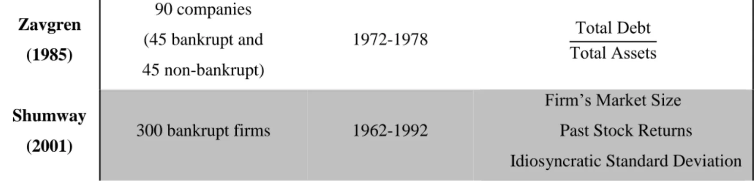
According to Correia (2012), Zavgren (1985) criticized the model of Ohlson, for having a theoretical basis for constructing the model somewhat weak as well as the study itself criticized for not having a paired sample. Consequently, Zavgren used the Logit technique with the objective to develop and test a new model of bankruptcy prediction able to identify the signs and estimate the probability of insolvency, five years before its occurrence by applying it to a sample of manufacturing firms in U.S.A..

Zavgren, used a sample of 45 bankrupt and 45 non-bankrupt firms and identified seven variables that were used to predict the future financial performance of businesses.

1. urrent ssets Inventories/ urrent iabilities 2. ebts/stocks

3. tocks/ ales

4. ash-Flow/ otal assets 5. ebt/ ssets

20 7. et ales/ et Fi ed ssets

Zavgren found evidence that financial ratios are significant measures in assessing the risks of insolvency and are more significant in the long-term efficiency ratios. He concluded that liquidity indicates that insolvent companies are more interested in liquidity than investment opportunities a year before the bankruptcy, with a negative sign. The debt was evidenced as a significant feature being that insolvent companies show higher levels of debt to healthy companies. However, measures of profitability were not significant to discriminate between healthy and bankrupt companies.

According to Chulwoo Han et all (2011), more recently, Shumway (2001) shows a Hazard Model. This model provides a more consistent estimate of failures compared to static models.

The dependent variable in a hazard model is the time spent by a firm in the healthy group. When firms leave the healthy group for some reason other than bankruptcy (e.g., merger), they are considered censored, or no longer observed. Shumway utilized accounting ratios and market variables, and showed that its forecasting power was superior to earlier models when tested in an out-of-sample period.

Shumway (2001) used a dataset of 300 bankruptcies (1962-1992), for which hazard models yield solid forecasting results. He concludes that market variables such as a firm’s market size, past stock returns, and the idiosyncratic standard deviation of its stock returns are found strongly related to default.

Based on previous studies, it makes sense that the analysis of that study focused some conclusions of other authors.

21

Author Sample Period in analysis Best predictive variables

Fitzpatrick (1932) 38 companies (19 bankrupt and 19 non-bankrupt) 1920-1929 uity ssets et income uity Beaver (1966) 158 companies (79 non-bankrupt and 79 bankrupt) 1954-1964

orking apital Funds otal assets et Income otal ssets Altman (1968) 66 companies (33 non-bankrupt and 33 bankrupt) 1946-4965 urrent ssets otal ssets etained earnings otal assets otal ssets arket alue of hares

otal ebt ales otal ssets Altman et all. (1977) 111 companies (53 bankrupt and 58 non-bankrupt) 1969-1972 umulative profitability etained arnings otal ssets Ohlson (1980) 2163 companies (105 bankrupt and 2058 non-bankrupt) 1970-1976 i e otal ssets otal liabilities total assets

Dummy variable, assume 1 if total liabilities exceeds total a

ssets, and 0 otherwise. et income otal assets

Funds provided by operations otal iabilities

I_t I_t | It| I_t

22 Zavgren (1985) 90 companies (45 bankrupt and 45 non-bankrupt) 1972-1978 otal ebt otal ssets Shumway (2001) 300 bankrupt firms 1962-1992 Firm’s arket i e Past Stock Returns

Idiosyncratic Standard Deviation

23

3. Methodology

3.1 Logit Model

The Logit model is a conditional probability technique used to study the relationship between a series of characteristics of an individual (or company) and its likelihood to belong to previously established groups (Lizarraga, 1997). As referred previously, the fundamental characteristic of logit model is that dependent variable can only assume a value of 0 or 1 (dichotomic variable4).

In order to estimate the parameters of the model, the maximum likelihood method5 is used. The maximum likelihood estimation is one of several alternatives6 approaches that statisticians have developed for estimating the parameters in a mathematical model. This method can be applied in the estimation of complex nonlinear as well as linear models.

There are many multivariate statistical techniques used to predict a dichotomous dependent variable from a set of independent variables, such as the discriminant analysis.

The linear discriminant analysis allows a direct prediction of the group to which the variable belongs - bankrupt / not bankrupt. However, despite being an optimal prediction rule, this technique requires the assumption of multivariate normality of the independent variables and matrices of variance - covariance equals in both groups.

In the logit model there are no restrictions about the normality of the explanatory variables. Therefore, it seems less restrictive to apply it. When applied to the Logit model, the

4 _{The dependent variable is called dummy variable. Dummy variables are also known as qualitative variables}

because they are often used to numerically represent a qualitative characteristic of an entity. Dummy variables are usually specified to take on one of a narrow range of integer values, and in most instances only zero and one are used.

Dummy variables can be used in the context of cross-sectional or time series regressions.

5 _{The maximum likelihood function estimates and associated standard errors of the regression coefficients in a}

logistic model are typically obtained by using computer packages for logistic regression. These statistics can then be used to obtain numerical values for estimate adjusted odds ratios, to test hypotheses and to obtain confidence intervals for population odds ratios based on standard maximum likelihood techniques.

6 _{Another popular approach is least squares estimation. This approach as a method for estimating the parameters}

in a classical straight line or multiple linear regression mode. These two methods are different approaches that happen to give the same results for classical linear regression analyses when the dependent variable is assumed to be normally distributed.

24 main objective of maximum Likelihood estimation method is to find the value of the parameters and that maximize the probability given by likelihood function.

Thus, in the Logit model, the relation between the probability of a business failure (p) and the value of the financial ratios is a curve in S ranging between 0 and 1.

The logistic model is popular because it relates to the general sigmoid shape of the logistic function. A sigmoid shape is particularly appealing to epidemiologists, for example. If the variable is viewed as representing an index that combines the contributions of several risks factors, so that ( ) represents the risk for a given value of Z. In that way, the risk is minimal for low Z values, rises over a range of intermediate values of Z, and remains close to 1 once Z gets large enough.

The function of a logit model is based on a logistic cumulative probability function specified as:

( ) ( ∑ )

∑

Equation 1: Logistic model

In which:

∑

Equation 2: Logistic regression model Graph 2: Logit transformation

25

: Probability of bankruptcy

: Observation number

: Coefficient for each of the independent variables : Ratios of economic-financial companies

The parameters in equation determine the rate of increase or decrease of the S-shaped curve for ( ). The sign of parameter indicates whether the curve ascends ( ) or descends ( ), and the rate of change increases as | | increases.

When , the right-hand side of equation 1 simplifies to a constant. Then, ( ) is identical at all , so the curve becomes a horizontal straight line.

Equation 1 is well-suited to modeling a probability, since the values of ( ) range from 0 to 1 as varies from to .

The probability of bankruptcy is obtained through the product of the ratios and a Z index, which transforms the previous expression, allowing for a certain probability of bankruptcy. The explanatory variables with a negative coefficient decrease the probability of bankruptcy because they reduce to zero. Likewise, the independent variables with a positive coefficient increase the probability of bankruptcy.

The Logit methodology can present several problems:

 It require that the groups that are clearly well separated;

 It requires that the explanatory variables are independent; However, it also has some advantages:

 It does not assume a linear relationship between the dependent and independent variables;

 Does not require the variables to follow a normal distribution;

 It is more robust than discriminant analysis, since it is applicable other than the normal distribution;

26

 The dependent variable can be interpreted as the probability of the company going to insolvency.

 Appealing S-shaped description of the combined effect of several risk factors on the risk for a happening.

3.2 Independent variables

In what methodology is concerned, it is important to specify the utilization of the ratios. Financial ratios are a useful tool in interpreting financial statements. The information derived from the analysis of the financial data is relied on heavily by investors and managers. According Manley (1999), there are four main categories of financial ratios: (1) Liquidity, (2) Profitability, (3) Leverage, and (4) Activity/Efficiency.

Manley (1999), states that it is important to remember that when using financial ratios to assess the overall financial stability of a company, more than one ratio should be considered when formulating an accurate opinion, because, for example, a company's solvency ratios may be ideal, but if the ratios that help analyze profitability and activity are bad (profits are down and sales are stagnant), a much different opinion would be formulated.

Bearing that explanation in mind, the ratios will support the probability of default, making it important to cover the analysis of liquidity, activity, debt and profitability. As mentioned before, the choice of the independent variables is based on some conclusions of other authors.

The ratios studied are: profit margin, asset turnover, ROA, financial leverage, ROE, Debt index, interest coverage ratio and general liquidity. These ratios are qualified in the areas mentioned (liquidity, activity, debt and profitability).

ROE, ROA and Asset Turnover are profitability ratios. Return on equity (ROE) measures a corporation's profitability by revealing how much profit a company generates with the money shareholders have invested. This means the amount of net income returned as a percentage of shareholders equity.

27

( )

An indicator of how profitable a company can be is its total assets. ROA gives an idea of how efficient the management is at using its assets to generate earnings. This ratio can be considered the most important in corporate finance. It measures percentage returns delivered to shareholders. A good number brings success to the business, making it easier to attract new funds. New funds will enable the company to grow with favorable market conditions, and this, in return, leads to higher revenues. All of this leads to a high value and continued growth of the wealth of the owners. ROA is calculated by dividing a company's annual earnings by its total assets and it is displayed as a percentage. Sometimes this is referred to as "a return on investment".

( )

The asset turnover ratio (AT) indicates the efficiency in the use of company assets. It should be compared between firms in the same industry and can assume different values between them. Asset turnover measures a firm's efficiency in using its assets for generating sales or revenue - the higher the number, the better. It also indicates that companies with low profit margins tend to have high asset turnover, while those with high profit margins have low asset turnover.

( )

When it comes to activity, the ratio calculated is Profit Margin (PM) and it is very useful to compare companies in similar industries. A higher profit margin indicates a more profitable company that has better control over its costs when compared to its competitors. This ratio is closely related to the pricing policy of the company and the gross margin that this reserve on the cost price of the goods sold.

( )

About debt ratios, the debt coverage ratio (CI) is a financial ratio that measures the risk and the ability of an entity to satisfy their financial commitments. This ratio relates the financial interest that the company supports, with the operating income it generates. When the

28 ratio is higher, the likelihood to generate sufficient operating income to meet the financial obligations money is higher too.

( )

Total debt to total assets, Debt Index Ratio (DI) is a leverage ratio that defines the total amount of debt relative to assets. The higher the ratio, the higher the degree of leverage, and consequently, financial risk (the higher the value gets, the higher the company becomes vulnerable). This is a broad ratio that includes long-term and short-term debt (borrowings maturing within one year), as well as all assets – tangible and intangible.

( )

Leverage ratios measure how leveraged a company is, and a company's degree of leverage is often a measure of risk. When the debt ratio is high, for example, the company has a lot of debt relative to its assets. About Debt-to-Equity (D/E), this ratio indicates the relationship between liabilities and equity, or the ability of the company to meet its obligations exclusively with equity.

( )

To cover all the management areas, it is also necessary to introduce the liquidity ratios. Liquidity (L) is a general representation of the working capital7 and has great importance to lenders.

If liquidity is higher than 1, it means that current assets are higher than short term debts making working capital positive.

7

Liquidity can be analyzed with the help of working capital. Working capital is often touted as a "safety pillow" of the company when lenders claim repayments of short-term debt.

Working capital is the excess of current assets in relation to short-term debt. It represents the part of current assets not financed by short-term debts, but by the permanent capital (debt over the medium and long term and equity). A company has liquidity when its working capital is sufficient to face risks arising from the slowness with which the assets turn into cash. When this does not happen imbalances in the treasury may happen.

29 If Liquidity equals 1, current assets are equal to short-term debts, in this case working capital is zero. It is important for the manager to keep track of this situation because the treasury of the company is unstable.

If Liquidity is lower than 1, current assets are worth less than short-term debts, leading to negative working capital.

( )

30

4. Empirical Study

4.1 Selection of the sample

As mentioned before, this study focuses on the civil construction between 2000 to 2012.

According to data obtained by the IIC, “Instituto de Informação ao Consumidor”, in 2011 there were 3312 cases of insolvency, among which 642 were companies in the construction industry. In the last few years, this value has increased even more, and is compounded at 48%, corresponding to 4902 cases, of which 982 are in the sector in question.

According to the “Federação Portuguesa da Indústria de Construção e Obras

Públicas”, the construction industry had been in a recession since 2002 as a result of a lack of

investment. This is a major factor contributing to the lack of growth in the Portuguese economy. Therefore we can confirm that crisis is not a direct result of the health of the construction industry but it is seriously aggravated by it.

Analyzing the values of the investment survey in April 2012 (INE), the internally generated funds remain the main source of financing for investment. Regarding construction, it can be noted that the internally generated funds represents 68.8% of the way construction companies were financed in 2011 leaving 25.7% for bank loans and 5.4% for other forms.

The past year showed a scenario not much different and, as expected, the option to resort to bank loans dropped to 24% leaving self-financing with 68.3% and 7.7% with other forms. In this survey other possible sources were suggested such as EU funds, stocks and bonds and even state loans, but without positive results.

he most important uestion to ask at this point is: “ his investment didn´t happen, why?” he answer is simple; most of these companies do not see the sale prospects increasing and do not believe in the profitability of investments, worse still, they know how reluctant banks have become in accepting loan requests.

It is, therefore, possible to identify the main reasons why so many companies become bankrupt, namely: the constraints on access to credit; shrinking margins in the business; and

31 delays in payments from the state. To prevent these situations, the goal is estimate the probability of the company becoming bankrupt using forecasting models.

With help from “IGNIOS - Gestão Integrada de Risco S.A”, some data was obtained from 20 insolvent enterprises and 25 solvent enterprises. This data refers to balance sheets and income statements of the companies.

These values are annual and data includes figures from the 3 years prior to the declaration of the company’s bankruptcy date.

To estimate Logit Model it is necessary to compute the ratios, but, first it is important to define the dichotomous dummy variable. As described in methodology, this variable can only assume a value of 0 or 1, so, for the development of this study, 0 stands for the non-bankrupt firms and 1 stands for non-bankrupt firms.

In order to estimate the parameters of the logit model the first step is to compute the ratios which are considered the explanatory factors of the probability of default.

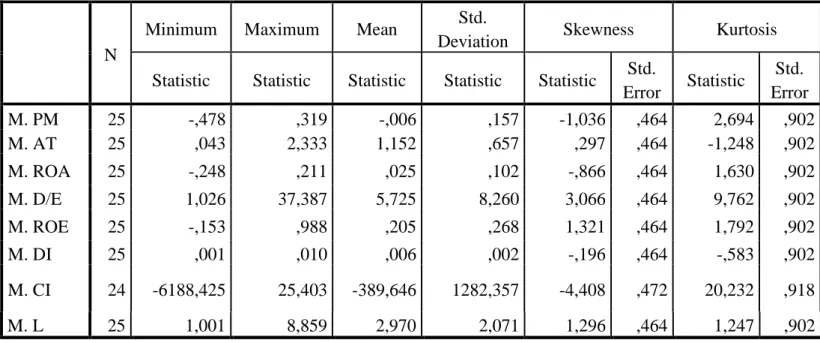
To this end, we resorted to a sample of 45 companies (25 non-bankrupt firms and 20 bankrupt firms) and calculated an average of all the years under review possible to calculate the ratios, and the conclusions for the solvent companies are present next.

N

Minimum Maximum Mean Std.

Deviation Skewness Kurtosis

Statistic Statistic Statistic Statistic Statistic Std.

Error Statistic Std. Error M. PM 25 -,478 ,319 -,006 ,157 -1,036 ,464 2,694 ,902 M. AT 25 ,043 2,333 1,152 ,657 ,297 ,464 -1,248 ,902 M. ROA 25 -,248 ,211 ,025 ,102 -,866 ,464 1,630 ,902 M. D/E 25 1,026 37,387 5,725 8,260 3,066 ,464 9,762 ,902 M. ROE 25 -,153 ,988 ,205 ,268 1,321 ,464 1,792 ,902 M. DI 25 ,001 ,010 ,006 ,002 -,196 ,464 -,583 ,902 M. CI 24 -6188,425 25,403 -389,646 1282,357 -4,408 ,472 20,232 ,918 M. L 25 1,001 8,859 2,970 2,071 1,296 ,464 1,247 ,902

32 Looking for the table 3 and taking to attention standard deviation it’s possible to see that the mean coverage ratio shows the highest value. This value means that there is a big dispersion among the data of each company. Analyzing the M. Debt Index and M, Profit Margin, shows a value close to zero, and when this happens it’s possible to affirm that there are no dispersion between the data for each firm.

Analyzing the measure of skewness8, it’s possible to see if the distribution of frequencies is skewed or asymmetric.

Taking for basis a significant level of 10%, can affirm if the coefficient of asymmetric take the value between -1.645 and 1.645 the distribution is symmetric. If the value is higher than 1.645 (with the same significant level) the distribution is positive asymmetric and if the coefficient is lower than -1.645 the distribution is negative asymmetric, verifying a predominance of higher values of the variable.

Observing the values of the table 3 just the ratio Mean Debt-to-Equity assumes a value higher than 1.645 (positive asymmetric). Otherwise, there are four ratios that assume a negative asymmetric distribution, so it is possible to support that there are a predominance of lower values of the variables.

Exploring the excess of kurtosis9, and taking to consideration the results observed in standard deviation, considered that the distribution is mesokurtic (with the same flatness of the normal distribution) if the coefficient of kurtosis assumes a value between -1.645 e 1.645 with the level of significance of 10%. If the coefficient of kurtosis is higher than 1.645 (level of significance of 10%) the distribution is leptokurtic, this means that the distribution of frequencies are more concentrate. On the other hand, if the value of coefficient is lower than -1.645 (with the same level of significance) the distribution is platykurtic, i.e., the shape of the frequency distribution curve is flatter (more dispersed). As mentioned before, and taking to account the results achieved by standard deviation, the ratio debt index, shows a standard deviation nearly to zero and a coefficient of kurtosis is -0.5829, this value are comprehended between the interval of the mesokurtic distribution, so the distribution has the same flatness of normal distribution.

8

Formula of asymmetry coefficient = _{( )( )} ∑ ( ̅)

9 _{Formula of skewness coefficient:} ( ) ∑ ( ̅) ( )

33 Analyzing the other coefficients of excess of kurtosis, all the values shows a mesokurtic or leptokurtic distribution, this means that distribution follows the normal distribution or the shape of the frequency distribution curve is more slender (more concentrated).

When observing the maximum and minimum of M. Debt Index of non-bankrupt firms, the values are nearly close to zero; the relation between debts and assets is practically null.

Relatively to maximum of M. Profit Margin, it is possible to see that even the companies considered healthy did not show a good value of profit. The maximum mean value presented in non-bankrupt firms is just 0.319.

4.2 Results of solvent companies

Observing now the mean of each independent variable, and focusing primarily in the values obtained, for the ratios of solvent companies and in the M. Profit Margin, we can conclude that the average value is negative but very close to zero (-0.00591). When it comes to the analysis of companies considered healthy, it makes sense that this value is positive or close to zero. -0,6 -0,4 -0,2 0 0,2 0,4 1 2 3 4 5 6 7 8 9 10 11 12 13 14 15 16 17 18 19 20 21 22 23 24 25

Solvent Companies - Profit Margin

Profit Margin Mean Profit Margin

Graph 3: Mean of solvent companies, profit margin analysis. Source: Author

34 -0,3 -0,2 -0,1 0 0,1 0,2 0,3 1 2 3 4 5 6 7 8 9 10 11 12 13 14 15 16 17 18 19 20 21 22 23 24 25

Solvent Companies

ROA Mean Roa 0 0,5 1 1,5 2 2,5 1 2 3 4 5 6 7 8 9 10 11 12 13 14 15 16 17 18 19 20 21 22 23 24 25

Solvent Companies - Asset Turnover

Asset Turnover Mean Asset Turnover

Looking now to the graph 4, it is visible that the asset turnover value with an average value equals 1.1521.

Graph 4 shows that there are more companies with asset turnover below average. This may be a sign of potential for sales that is not being maximized, the scarcity of derivative assets. On the other hand, firms located above average, convey that companies have excess capital when compared to their real needs.

In order to understand what these companies can do with their assets it is necessary to take the ratio of profitability into consideration. The average value for M. ROA is 2.49%, which means that on average the applied assets are 2.49% profitable.

Graph 4: Mean of solvent companies, asset turnover analysis. Source: Author

Graph 5: Mean of solvent companies, ROA analysis. Source: Author

35 When investigating bankrupt situations, it is important to analyze liquidity ratios.

Ratio Mean Non-Bankrupt Companies

M. Liquidity 2.967

Table 4: Mean solvent companies, liquidity ratios.

As mentioned above, when liquidity ratio is positive, working capital follows the same trend, ie, greater than zero. This liquidity ratio transmits some security to the creditors of the company. The realization of current assets for liquidity is sufficient to meet the short term debts and the company still has some safety margin.

4.3 Results of insolvent companies

Analyzing now the values for a sample of 20 insolvent companies, data are present below.

N

Minimum Maximum Mean Std.

Deviation Skewness Kurtosis

Statistic Statistic Statistic Statistic Statistic Std.

Error Statistic Std. Error M. PM 17 -1,793 ,247 -,362 ,582 -1,716 ,550 2,266 1,063 M. AT 17 ,039 5,077 1,416 1,451 1,780 ,550 2,334 1,063 M. ROA 20 -1,316 ,205 -,201 ,329 -2,260 ,512 6,598 ,992 M. D/E 20 -10,187 33,290 3,292 8,679 2,106 ,512 7,424 ,992 M. ROE 20 -2,127 5,986 ,283 1,513 2,827 ,512 11,569 ,992 M. DI 20 ,000 5,451 ,965 1,339 2,318 ,512 6,265 ,992 M. CI 20 -3442,178 178,579 -223,694 783,602 -4,052 ,512 17,059 ,992 M. L 20 ,148 1840,623 95,538 410,866 4,468 ,512 19,974 ,992

36 -3 -2 -1 0 1 2 3 4 5 6 1 2 3 4 5 6 7 8 9 10 11 12 13 14 15 16 17 18 19 20

Bankrupt Firms - Profit Margin VS Debt Index

Profit Margin Debt-to-Equity

When analyzing table 5 and the standard deviation, it’s possible to see that the two highest values are mean coverage ratio (783.602) and mean liquidity (410.866). With these values, it is possible to confirm that there is a lot of dispersion between the data of each company. About other standard deviation values, the values are very similar (excluding mean financial leverage (8.679) and the lower is mean profit margin (0.582), so it can be said that in the other independent variables there is no dispersion between the data.

In order to support the conclusions of standard deviation and based on the explanation of the excess of kurtosis in the solvent companies, all of the kurtosis coefficients are higher than 1.645, so it can be said that all the independent variables follow a leptokurtic distribution, the shape of the frequency distribution curve is more slender (more concentrated), i.e., there is not a lot of dispersion, with a level of significance of 10%.

About skewness, with a level of significance of 10%, just M. Profit Margin (-1.716), M. ROA (-2.260) and M. Coverage Ratio (-4.052) are classified as asymmetric negative distributions, while all the others are positive asymmetric distributions, this means that there is a predominance of lower values of the variables.

The analyses of the mean ratios of the insolvent companies showed us that the average of Profit Margin is -0.362. As expected, this ratio is negative, which means that on average firms' profitability is negative (ie, do not generate profit). Generally, we have a low margin profit when we are dealing with an inappropriate financial structure which leads to high financial, harmful costs to the profitability of the total investment.

Graph 6: Mean insolvent companies, profit margin vs debt index analysis. Source: author

37 0 0,5 1 1,5 2 2,5 3 3,5 4 4,5 5 5,5 1 2 3 4 5 6 7 8 9 10 11 12 13 14 15 16 17 18 19 20

Bankrupt Firms - Asset Turnover

Asset Turnover Mean Asset Turnover

These two ratios assume a general inverse relationship, as can be seen in graph 6. When one of them increases the other one tends to decrease. This makes sense because when the debt index has a very high value, the profit margin tends to decrease.

It becomes essential to analyze M. ROE once it is one of the most important indicators of the profitability and efficiency of management. This ratio measures the rate of recovery (or return) of investment, obtained by the holders of the shares. It shows the percentage of investment the owners have done in the business, obtained through profit annually.

Presenting a value of 28.3%, M. ROE compares profits achieved in the accounting period with the amount invested in the same period by the owners. It is considered that this rate of return is low, which may indicate that this capital is not being correctly invested. We can prove this by analyzing the ROA.

Profitability ratio has also a negative value -20.1%. This means that in average, the assets are at a loss to 20.12 % of its profitability.

Regarding the M. Asset Turnover, it represents a very similar value of solvent companies, 1.416. As mentioned earlier, this ratio expressed how efficiently the company uses its assets to generate profitable sales. It measures the overall effectiveness of management in the use of total investment. As with the solvent companies, we can see through the graph below, that there are more companies below the industry average. This means that companies are not generating adequate sales volume to investments held.

Graph 7: Mean insolvant companies, asset turnover analysis. Source: Author

38 Finally, we should look back to the liquidity of bankrupt firms.

Ratio Mean Non-Bankrupts Companies

M. Liquidity 95.538

Table 6: Mean insolvent companies, liquidity analysis

On average, these companies can liquidate 95.54% of its current assets. It’s important to refer that the high value, it cannot always be considered a good sign, because it can mean that companies are not effectively using their short-term assets. This happens because, as mentioned above, the company has a low asset turnover (existence of more values below the industry average). From the moment this happens it may become difficult for companies to meet short-term obligations.

39

4.4 Correlation of the sample variables

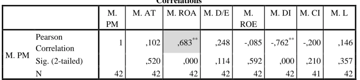
Starting now to examine the correlation among the predictor variables, it can be concluded that there is not a strong correlation between the ratios.

ooking to table 7, it’s possible to see that there are coefficients statistically significant to 1% and 5%. We can observe moderate correlation when Mean Profit Margin vs Mean ROA. With the help of SPSS, we achieve the Pearson correlation of 0.683. These correlations are statistically significant for a 1% significance level.

Table 7: Correlations between independent variables

Turns out obvious that must exist some correlation between these ratios because they are activity and profitability ratios. These two ratios are all related and “walk in the same direction”, if we have high profit margin these means that the assets of companies are being well spent, and consequently generating a high ROA.

Observing the correlation between Mean D/E and Mean PM, it is visible that there is a correlation of 24.8%, however, this value is not statistically significant (0.114%). Taking into account the entire explanatory variable and the significance value for each one, almost of the ratios are not 5% statically significant.

Looking now at the negative correlations there are too coefficients statistically significant to 1% and 5%. Correlations M. PM M. AT M. ROA M. D/E M. ROE M. DI M. CI M. L M. PM Pearson Correlation 1 ,102 ,683 ** ,248 -,085 -,762** -,200 ,146 Sig. (2-tailed) ,520 ,000 ,114 ,592 ,000 ,210 ,357 N 42 42 42 42 42 42 41 42

**. Correlation is significant at the 0.01 level (2-tailed). *. Correlation is significant at the 0.05 level (2-tailed).

40 Based on table 8, we find that with a Pearson coefficient of -0.762 for Mean Profit Margin vs Mean Debt Index, and -0.780 for Mean ROA vs Mean Debt Index. These two correlations are statistically significant for a 1% significance level.

Correlations M. PM M. AT M. ROA M. D/E M. ROE M. DI M. CI M. L M. PM Pearson Correlation 1 ,102 ,683 ** ,248 -,085 -,762** -,200 ,146 Sig. (2-tailed) ,520 ,000 ,114 ,592 ,000 ,210 ,357 N 42 42 42 42 42 42 41 42 M. ROA Pearson Correlation ,683 ** -,286 1 ,208 -,168 -,780** -,017 ,053 Sig. (2-tailed) ,000 ,066 ,170 ,269 ,000 ,912 ,729 N 42 42 45 45 45 45 44 45

**. Correlation is significant at the 0.01 level (2-tailed). *. Correlation is significant at the 0.05 level (2-tailed).

Table 8: Correlations between independent variables.

Considering all negative correlations, only the two mentioned above and M. D/E vs M. DI and M. ROA vs M. AT are 1% and 5% statistically significant10. All the other explanatory variables didn’t show a statically significant level.

10

41

5 Estimation of the model

5.1 The Logit

The table below shows that only 41 companies are being studied once 4 are classified as missing cases.

Case Processing Summary

Unweighted Casesa N Percent

Selected Cases Included in Analysis 41 91,1 Missing Cases 4 8,9 Total 45 100,0 Unselected Cases 0 ,0 Total 45 100,0

a. If weight is in effect, see classification table for the total number of cases.

Table 9: Sample

Considering the 45 firms, and for the estimation process, 24 have been considered as solvent firms and 17 as insolvent firms.

Classification Tablea,b

Observed Predicted Dummy Percentage Correct 0 1 Step 0 Dummy 0 24 0 100,0 1 0 17 ,0 Overall Percentage 58,5

a. Constant is included in the model. b. The cut value is ,500

42 The table above shows that the forecast of the company to be solvent is correct in 58.5% while the prediction of it to be insolvent is 41.5%.

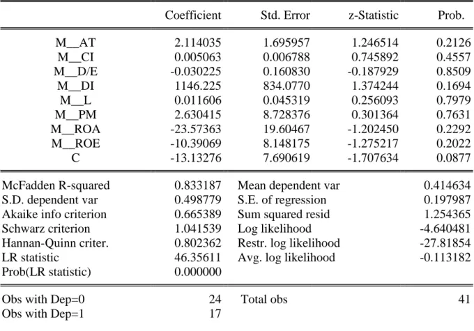
Table 11 indicates the explanatory variables used in the logit model and the estimation results through EViews. The estimates for the parameters, Z-statistics and their significance levels are also presented in the next table.

Coefficient Std. Error z-Statistic Prob.

M__AT 2.114035 1.695957 1.246514 0.2126 M__CI 0.005063 0.006788 0.745892 0.4557 M__D/E -0.030225 0.160830 -0.187929 0.8509 M__DI 1146.225 834.0770 1.374244 0.1694 M__L 0.011606 0.045319 0.256093 0.7979 M__PM 2.630415 8.728376 0.301364 0.7631 M__ROA -23.57363 19.60467 -1.202450 0.2292 M__ROE -10.39069 8.148175 -1.275217 0.2022 C -13.13276 7.690619 -1.707634 0.0877

McFadden R-squared 0.833187 Mean dependent var 0.414634

S.D. dependent var 0.498779 S.E. of regression 0.197987

Akaike info criterion 0.665389 Sum squared resid 1.254365

Schwarz criterion 1.041539 Log likelihood -4.640481

Hannan-Quinn criter. 0.802362 Restr. log likelihood -27.81854

LR statistic 46.35611 Avg. log likelihood -0.113182

Prob(LR statistic) 0.000000

Obs with Dep=0 24 Total obs 41

Obs with Dep=1 17

Table 11: Logit Model, with all independent variables

Through this table, the estimation results point for a high McFadden value (0.833187).

Regarding the parameters showed in the table above, it is possible to achieve the estimates for the coefficients showed in equation 2. Thus, the estimation equation is given by:

( ̂ )

̂