MSC IN FINANCE
MASTER FINAL WORK
DISSERTATION
ACTIVE VERSUS PASSIVE MANAGEMENT: THE
CASE OF BOVESPA
JUNIOR GABRIEL FARIA DE SOUSA
MSC IN FINANCE
MASTER FINAL WORK
DISSERTATION
ACTIVE VERSUS PASSIVE MANAGEMENT:
THE CASE OF BOVESPA
JUNIOR GABRIEL FARIA DE SOUSA
Supervisor:
MESTRE TIAGO RODRIGO ANDRADE DIOGO
Jury:
PROFESSORA DOUTORA RAQUEL MARIA MEDEIROS GASPAR MESTRE TIAGO RODRIGO ANDRADE DIOGO
MESTRE VICTOR MAURILIO SILVA BARROS
ii
ABSTRACT
The main purpose of this paper is to analyze some models underlying the active and passive portfolio management and what would be its impact on the choice of a portfolio composed by stocks which are integrated in BOVESPA Index, Brazilian biggest stock market. We will test if, for 1 year and 2 years “data winbdows”, there are significant differences, in terms of annualized daily returns and Sharpe ratio, between the different portfolios treated on the dissertation, in order to find which one we should choose.
The passive management approach is based on the historical prices of BOVESPA Index which replicates the behavior of the market and on the naïve method (1/N), in which the portfolio includes all the stocks on the index with the same proportions. Active management is based on the Markowitz model, also known as mean variance model, whose objective is to maximize the return give a set risk level or, minimize the risk given an expected return. The minimum variance model is also used, whose goal is to minimize the risk independent of the return. On these approach the weights of each asset in the portfolio are revised monthly, based on the market evolution. Another model used is a Mean Variance adjusted method in which the first period optimal weights will be maintained for the remaining data windows. In order for these to be determined, “windows” of 1 and 2 years were used. The data were taken from Datastream and we are considering a 10 year investment horizon, from January 2005 to December 2014.
Based on the results, we can affirm that the mean variance portfolio should be chosen, as performed better both in terms of returns and , especially, in terms of Sharpe ratio when compared with the other two portfolios.
JEL: G11
Keywords: Active Management, Passive Management, Portfolio Shares, Markowitz Model, Minimum Variance Model, Equity Portfolio with Equal Weights, Sharpe ratio.
iii
RESUMO
O principal objetivo deste trabalho é analisar alguns modelos subjacente à gestão de carteiras ativa e passiva e qual seria seu impacto sobre a escolha de uma determinada carteira constituída por ações que estão integrados no índice BOVESPA, maior mercado bolsista do Brasil. Para isso foi analisado se, para janelas de dados de 1 e 2 anos, existem ou não diferenças significativas entre as carteiras em consideração, com a finalidade de saber se é possível se, para rendibilidades e rácios de Sharpe mais elevados, escolher a melhor carteira entre aquelas analisadas.
A gestão passiva é baseada numa carteira que visa replicar o comportamento do Índice BOVESPA, tendo como base os preços históricos do índice e no método naïve (1/N), no qual composição da carteira inclui todos os ativos do índice com as mesmas proporções. A gestão ativa baseia-se no método de Markowitz, conhecido como modelo de média variância, que visa maximizar o retorno tendo definido um determinado nível de risco, ou minimizar o risco tendo em conta um nível de retorno esperado. Também é usado o método da variância mínima que consiste em minimizar o risco independentemente do retorno. Nesta abordagem as proporções a investir em cada ativo são revistas mensalmente tendo em conta a evolução do mercado. Outro modelo utilizado será um método ajustado da média variância em que serão mantidos os pesos ótimos do primeiro período para as restantes janelas de dados. Para as determinar são consideradas “janelas” de dados de 1 e 2 anos. Os dados foram obtidos a partir do Datastream e é considerado um horizonte de investimento de 10 anos, a partir de Janeiro de 2005 a Dezembro de 2014.
Com base nos resultados é possível afirmar que a carteira de média variância deve ser a escolhida, uma vez que apresenta os melhores resultados.
JEL: G11
Palavras-chave: Gestão Activa, Gestão Passiva, Portfolio de Acções, Modelo de Markowitz, Modelo de Variância Mínima, Carteira de Acções com Pesos Iguais, Rácio de Sharpe.
iv
Contents
1 INTRODUCTION ... 1 1.1. OVERVIEW ... 1 1.2. PURPOSE ... 2 1.3. STRUCTURE ... 3 2 LITERATURE REVIEW ... 4 2.1. INTRODUCTION ... 42.2. THE MODERN PORTFOLIO THEORY ... 4
2.3. NAIVE PORTFOLIO AND MINIMUM VARIANCE PORTFOLIO ... 10
2.4. ACTIVE AND PASSIVE PORTFOLIO MANAGEMENT ... 12
2.5. PERFORMANCE EVALUATION ... 13
2.6. SHARPE RATIO ... 14
3 HYPOTHESIS ... 16
4 DATA AND METHODOLOGY ... 20
4.1. DATA ... 20
4.2. METHODOLOGY ... 20
5 RESULTS ... 25
5.1. PERFORMANCE OVERVIEW ... 25
5.2. HYPOTHESIS TESTS - RESULTS ... 26
6 CONCLUSION ... 30
6.1. MAIN CONCLUSIONS ... 30
6.2. LIMITATIONS AND FURTHER RESEARCH ... 31
7 REFERENCES ... 33
v
Tables List
TABLE 1 - Hypotheses tests, with 1 year “data window”... 25 TABLE 2 – Hypotheses tests, with 2 year “data window”... 26 TABLE 3 – Number of assets invested – mean variance portfolio for “1 year data
window”... 36 TABLE 4 – Number of assets invested – mean variance portfolio for “2 year data
window”... 36 TABLE 5 – Number of assets invested –minimum variance portfolio for “1 year data window”... 36 TABLE 6 – Number of assets invested – minimum portfolio for “2 year data
window”... 37 TABLE 7 – Number of assets invested –naive portfolio for “1 year data
window”... 37 TABLE 8 – Number of assets invested – naive portfolio for “2 year data
vi
Figures List
FIGURE 1 – Historical prices (2005 – 2014) –BOVESPA Index” ...34 FIGURE 2 – Returns – Mean Variance, Minimum Variance, Mean Variance Adjusted, Naive and BOVESPA Index portfolios (1 year “data windows”)………...37 FIGURE 3 – Returns – Mean Variance, Minimum Variance, Mean Variance Adjusted, Naive and BOVESPA Index portfolios (2 year “data windows”)………...38 FIGURE 4– Sharpe Index – Mean Variance, Minimum Variance, Mean Variance
Adjusted, Naive and BOVESPA Index portfolios (1 year “data windows”)……...38 FIGURE 5 – Sharpe Index – Mean Variance, Minimum Variance, Mean Variance
Adjusted, Naive and BOVESPA Index portfolios (2 year “data windows”)……...38 FIGURE 6- Volatility – Mean Variance, Minimum Variance, Mean Variance Adjusted, Naive and BOVESPA Index portfolios (1 year “data windows”)……...39 FIGURE 7 - Volatility – Mean Variance, Minimum Variance, Mean Variance Adjusted, Naive and BOVESPA Index portfolios (2 year “data windows”)……...39
vii
Acknowledgments
I am grateful to my supervisor, Prof. Tiago Diogo, for his guidance, insight and expertise that made the development of the work under this topic possible. I would also like to thank all my teachers who provided me the knowledge and tools required to complete my master’s dissertation.
I thank my parents for their education, support and for the values they taught me; my brothers, and the rest of my family and friends for their help in completing this stage.
1
1 Introduction
1.1. Overview
Nowadays, investors have at their disposal a wide variety of techniques and models in order to construct their portfolio. However the Modern Portfolio Theory, i.e. the Mean Variance Theory, introduced by Harry Markowitz in the 50´s, has had a major influence in the practice of portfolio management. It has introduced a whole new terminology which now has become the norm in the area of investment management. An important outcome of the research generated due to the ideas formalized in the mean variance model is that today’s investment professionals and investors are very different from those 50 years ago. Not only are they more financially sophisticated, but, additionally, they are armed with many more tools. This allows both investment professionals to better serve the needs of their clients, and investors to monitor and evaluate the performance of their investments.
The mean variance model is an active management portfolio technique, i.e. it does not aim to track a given benchmark or Index. Another model active portfolio managers could use is based on the minimum variance portfolio theory, which basically consists in the portfolio of risky assets that has the lowest possible variance, i.e. it is the optimal portfolio with lower risk (Bodie et al., 2009). . Another model used is a Mean Variance adjusted method in which the first period optimal weights will be maintained for the remaining data windows.
Further to the models above, the passive management approach is based on the historical prices of BOVESPA Index which replicates the behavior of the market and on the naïve method (1/N), in which the portfolio includes all the stocks on the index with the same
2
proportions. Regarding passive management models, there will be used two models, a model which replicates the Index and the naive model. The last model is composed by an equally weighted portfolio, being the proportion invested in each security equals to 1/N (N as the number of shares).
In 2015, Brazil was world’s fifth most populous nation, ONU (2015), and consequently an important emerging market economy. Over the last decades, and especially during the period under analysis (see figure 1 as reference) , Brazil’s stocks market has faced periods of bear and bull markets, affected by high levels of inflation, exchange rate volatility and high interest rates applied by the Brazilian Central Bank. Taking this into consideration, I believe it would be interesting and enriching to analyze BOVESPA Index, the behavior of the different portfolios and how the different models could help investors managing their portfolios.
1.2. Purpose
The main purpose of this paper is to analyze some models underlying the active and passive portfolio management and what would be its impact on the choice of a portfolio composed by stocks which are integrated in BOVESPA Index, Brazilian biggest stock market. We will test if, for 12 and 24 months, there are significant differences, in terms of annualized daily returns and Sharpe ratio, between the different portfolios treated on the dissertation, in order to find which one we should choose.
3
1.3. Structure
This dissertation is built in six main chapters. The first is composed by the current chapter, where an introduction to the subject is made. Then continues, in chapter 2, with the literature review, in which results from research and analysis of preview studies and written papers are exposed. The literature review is divided in 4 parts: mean-variance portfolio model, minimum variance and Naïve portfolios, active and passive management, and performance evaluation. In the third section testing hypotheses are introduced. While, data and methodology are discussed in the fourth section. In the fifth chapter the results obtained from the hypothesis tests are presented. At last, chapter 6 exhibits the work conclusions and refers limitations to it. It also points some future research that could be done.
4
2 Literature Review
2.1. Introduction
In this chapter we will review the literature related with portfolio theory, mean-variance model, active and passive portfolio management, performance evaluation and Shape ratio. The main goal of this section is to highlight, understand and explore all the ideas and results of the empirical research made on this subjects in the past, analyzing different point of views, starting on the research made by Markowitz over the years.
2.2. The Modern Portfolio Theory
Markowitz (1952) introduces the study of Portfolio Theory to the world, when he declares that the process of selecting a portfolio is divided into two components. The first commences with the observation and experience and terminates with the expectation around future returns of the available assets. The second component commences with the relevant expectations around the returns and risks of an asset, terminating with the choice of the portfolio. Markowitz assumed that all the investors were rational, i.e. all the investors were risk averse and pursuit higher profit. Based on that assumption, this theory provides a model to maximize the expected return of a portfolio for a certain level of risk, or minimize the risk of a portfolio for a given amount of expected return. This model illustrates the process of selecting optimal scenarios through efficient frontier and lowering risks by diversifying investment. It is also stated in the theory that, instead of simple collection of assets, investors should choose different assets with lower correlation coefficients.
5
The main goal of portfolio optimization is to find a combination of assets (xi: portfolio
weights of each asset) that minimizes the standard deviation of the portfolio return for any given level of expected return or, in other words, a combination of assets that maximizes the expected return of the portfolio for any given level of risk. Mean variance optimization developed by Markowitz (1952) can be used in order to determine how an investor allocates his wealth among securities. The proportion of securities in a portfolio depends not only on their means and variances, but also on the interrelationships or covariance. Thus, covariances between securities as well as returns and variances are calculated as input in portfolio optimization, Horasanli, Mehmet et al. (2007). They proposed the use of exponentially weighted moving averages and the generalised auto-regressive conditional heteroskedasticity technique in portfolio selection was applied to a selection of stocks from the Istanbul Stock Exchange market and then compared the result with optimal portfolio obtained by classical Markowitz theory. They concluded that at the same level of expected return, one can always have less risky portfolios by using exponentially weighted covariance matrices, because Markowitz (1952:91) pointed to a way for calculating reasonable μ and σ parameters and the exponentially weighted scheme provides a more efficient way to calculate these parameters and respond to stock market changes.
The empirical research made on the subject of portfolio choice has referred the Markowitz Mean-Variance portfolio theory as the most appropriated for risk averse people (if the normality distribution of portfolio’s return is accomplished). Bawa (1976) tested the mean variance model using monotonous utility functions with positive slope, applying it to risk averse, lower and neutral investors. He affirmed that the model could be applied to all types of investors, as long as the portfolio includes an asset with a highest return and volatility.
6
The process of choosing a portfolio, following the point of view of Markowitz is, according to Rubinstein (2002), very common between portfolio managers, in its construction and in its evaluation as well. Rubinstein claims that Markowitz is not the first person who mentions the concept of diversification. This topic had already been mentioned by Daniel Bernoulli in 1973. According to Markowitz, diversification reduces the portfolio risk. However, it does not erase the risk completely. Consequently, the expectations of portfolio return will remain consistent, even though the decrease of that risk. In Rubinstein (2002), the main idea of Markowitz’s work is to demonstrate that the individual risk of an asset is not required to be considerable for the investor. Nevertheless, he must consider the asset's influence in the portfolio's changes. Assets are mandatory to be evaluated as an all and not separately. This means that the decision of conserving a certain asset should not only be made by comparing the expected returns and its variance, moreover having into account other assets the same investor possesses. Conventional wisdom has always dictated not putting all your eggs in one basket. In more technical terms, this adage is addressing the benefits of diversification. Markowitz’s model quantified the concept of diversification by introducing the statistical notion of a covariance, or correlation.
Evan and Archer (1968) found that the risk reduction effect diminishes rapidly as the number of stocks increases, concluding that the gains from diversification are exhausted when a portfolio contains ten or more stocks. Statman (1987) suggested that diversification should be increased as long as the marginal benefits exceed the marginal costs. Those benefits are related with risk reduction and the cost associated with transaction costs. He used a 500 stock portfolio which can be levered through borrowing and lending. He assumed that an investor draws randomly from all stocks to form portfolios that differ in
7
the number of stocks but have identical expected returns. He concluded that a well-diversified portfolio of stocks must include, at least, 30 stocks for a borrowing investor and 40 for a lending investor. This result contradicts the researchers previously quoted. In his study the author reveals the idea that diversification should only increase to levels where the marginal benefits are superior to the marginal costs, in other words, the investor continues to acquire titles, with the purpose of portfolio diversification, until its costs do not exceed the earnings. Furthermore, it is also mentioned that marginal costs thrive faster than the marginal benefits underlying the diversification.
Gaumnitz (1969) aimed to analyze what was the optimal number of assets a portfolio should have to accomplish fully diversification. He used the Standard and Poor’s 425 Industrial Index as database, analyzing several portfolios generated from a statistical tool known as ANOVA (Analysis of Variance) and others statistical tests. He concluded that, in order to have a well-diversified portfolio, the optimal number of stock should be 20. He also found that, for a certain number of securities, adding an additional asset to the portfolio will not bring any considerable benefit for the investor,
The concept of Efficient Frontier was introduced by Markowitz in 1952, in which he explains that investors can choose – between a set of portfolio – the optimal portfolio, being the one with the lowest level of risk for a certain level of return. Therefore to increase portfolio’s return, the level of risk should increase. Markowitz pointed that the Efficient
Frontier expands when short-selling1 is allowed, due to the increase of combinations of
assets forming efficient portfolios. Pogue (1970) identified other factors/features affecting
1 Short selling (or "selling short") is a technique used by investors who try to profit from the falling price of a
stock. Borrowing a security (or commodity futures contract) from a broker and selling it, with the understanding that it must later be bought back (hopefully at a lower price) and returned to the broker.
8
the shape and the composition of the efficient frontier, for instance, financing policy or liquidity, transactions and tax costs. He found that with regarding to transaction costs, the efficient frontier would retract, leading to lowest levels of return. On the other hand, if short-selling is allowed and the investor obtains outside financing the efficient frontier will expand, i.e. will move to highest levels of return.
Moreover, initiating with Markowitz (1952), it is important to analyze the work published by Horasanli et. al. (2007), in which they assumed that the medium-variance model is out of phase from the reality of the market. In this respect, they presented solution demands
using two statistic tools - EWMA2 and GARCH3, for the realization of this study, 15 stocks
presented on Istanbul Stock Exchange (XU30 Index) were taken into consideration, on the period between 09/08/2005 and 30/12/2005. Therefore, it was concluded that, for the same amount of expected return, it is always possible to obtain less risk using covarience matrices weighted exponentially.
Levy and Markowitz (1979) tested the efficacy of the mean-variance model by studying the correlation between it and expected utility (EU). Their research had two main goals: to see how good mean variance approximation were for various utility functions and to test an alternative way of estimating EU from a distribution’s mean and variance. They found that the mean variance approximation was usually the most accurate. They also observed that mean variance approximations to EU are quite good for many Utility functions except those with extremely risk aversion. However, Simaan (1993) found that such investors will be satisfied if the mean variance model includes a risk-free asset. Levy and Markowitz (1979)
2
Exponentially Weighted Moving Average
9
assumed that if EU and f(E,V)4 were highly correlated, then f(E,V) would provide a near
maximum EU. The reason for performing a mean variance analysis, rather than a theorical EU analysis is related with the cost of feasibility. It is commonly more expensive to find an utility maximizing portfolio than to trace out an entire mean-variance approximation, as the only inputs required for a mean variance analysis are the mean, variance and covariance of the securities under analysis.
According to Markowitz (1959) EU will be approximately equal to a function of expected return [E[R]] and variance of return V, if the utility function can be approximated closely enough by a quadratic for a sufficiently wide range of returns. Markowitz (2012) mentioned three types of utility function maximization: explicit, mean variance approximate and implicit. Explicit EU maximization occurs when an utility function is given and analytical or numerical methods are used to find the portfolio that maximizes the expected value of this function. On the other hand, mean variance approximation occurs when a utility function is given and mean variance approximation to its EU is maximized. The author concludes that if some investors choose the mean variance efficient portfolio which is the best for him, then the investor has selected a portfolio that maximizes his EU. This is classified by Markowitz (2012) as “implicit” expected utility maximization. According to the author, there are several inconveniences and expenses regarding the maximization of expected utility, especially when it is compared with an implicit approximation or a mean variance approach. For instance, regarding parameter estimation, a mean variance model analysis only requires mean, variance and covariances of the securities under analysis, and because the parameters do not depend on the form of the probability distribution, a factor
10
model can substitute the individual variances and covariances. On the other hand, for explicit maximization of EU we have to determine what type of joint probability distribution generates return combinations, (r1, r2,.., rn), and must estimate the parameters for such a joint distribution. Accomplishing this can be very time consuming. Another drawback of the explicit approximation approach is that one must determine the investor’s utility function, as opposed to implicit EU maximization.
Grauer (1986) considers the efficacy of mean variance approximation to the power of logarithmic utility function when the investor can borrow all he wants at the risk-free rate,
as allowed in the Sharpe-Lintner CAPM (capital asset pricing model).5He reported negative
results unless constraints were added to the mean variance model to avoid bankruptcy. Pulley (1983) suggested that investors maximizing a certain mean variance function would hold virtually the same portfolio as investors maximizing expected logarithmic utility taking into account exact empirical distribution of security returns.
2.3. Naive Portfolio and Minimum Variance Portfolio
Further to the mean variance portfolio theory introduced by Markowitz there are alternative
models that can be used to construct a portfolio of assets. These are the 1/N portfolio5 (also
known as the naive portfolio) and the minimum variance portfolio. As mentioned above, both models will also be used in this dissertation.
According to Kritzman et al. (2010), the outperformance of the Naïve portfolio over the Mean-Variance portfolio proved in De Miguel et al. (2007) is explained by the very short time windows they used, which were insufficient to find an accurate estimate of the
11
expected return of the portfolios. The authors used 13 databases containing 1028 data series,
having built 50.000 stock portfolios between February 1926 and December 2008. Simplest models of expected return, which require no foresight, were used. The portfolios were grouped into 3 categories: asset class, beta and alpha. In each data set, was compared the performance of the estimated portfolio, 1/N portfolio and the optimized portfolio. The results showed that using simple, but plausible, estimates expected return, volatility and correlation, applied differently, the portfolio optimization can have a higher performance than portfolios that use 1/N strategy. Concluding, when investors adopt short-time investment horizon, they will get results that are not satisfactory.
Duchin and Levy (2009) analyzed the mean-variance portfolio and the naïve portfolio. Their study took place between 1996 and 2007 using monthly data from 30 industrial portfolios of Fama- French6, and it takes into account restrictions on short selling. The authors conclude that for small investors, the naive portfolio seems to be the right one. Nevertheless, the results demonstrate that for institutional investors holding portfolio with a larger number of assets, the mean variance model dominates naive model.
With regarding to the minimum variance portfolio, according to Bodie et al. (2009) it can be defined as the portfolio of risky assets that has the lowest possible variance, ie, it is the optimal portfolio with lower risk. The strategies related with the minimum-variance portfolio aim to obtain a highest performance using the risk management during periods of financial crisis. Furthermore, they are very used, because low volatility securities tend to
6 The Fama/French benchmark portfolios are rebalanced quarterly using two independent sorts, on size
(market equity, ME) and book-to-market (the ratio of book equity to market equity, BE/ME). The size breakpoint (which determines the buy range for the Small and Big portfolios) is the median NYSE market equity. The BE/ME breakpoints (which determine the buy range for the Growth, Neutral, and Value portfolios) are the 30th and 70th NYSE percentiles.
12
track or outperform the market. According to Chow et al. (1999) the minimum variance portfolio has been classified and analysed since the beginning of modern portfolio theory, as being a specific case of the mean variance portfolio theory.
Clarke et al. (2006) state that “the basic Markowitz (1952) prescription is to estimate expected returns and a covariance matrix for securities, and then to minimize the portfolio’s ex ante risk for any given expected return by adjusting security weights”. In the same paper they said that all portfolios in the efficient frontier are designed to minimize risk for a given level return, on the other hand the minimum variance portfolio minimizes risk without an expected return input. By building a minimum variance portfolio using a large set of US equity securities and examining the realized risk and return over a given period, the authors found that actual return of the minimum variance portfolio is higher than the market return. Furthermore, the risk is substantially lower compared also with the market risk and finally the Sharpe ratio (will be study further below) from the minimum variance portfolio was much highest than the market’s Shape ratio. The main feature of minimum variance portfolio is that the weights of the securities in the portfolio are independent from the expected returns underlying those securities. Their main conclusion was that while the portfolios that are on the efficient frontier are designed to minimize the risk for a given return, the minimum variance portfolio aims to minimize the risk regardless of the expected return.
2.4. Active and Passive Portfolio Management
In order to manage a portfolio, the investors can choose between two different management approaches: active and passive. According to Elton et al. (2011), the passive portfolio aims
13
to track a given benchmark, a stock Index for example, and the passive portfolio manager invest in a portfolio which replicate the benchmark. The naive portfolio (1/N) is one of the most common passive management approaches, and it could be defined as “a portfolio in which a fraction 1/N of wealth is allocated to each of the N assets available for investment” De Miguel et. al. (2007). On the other hand an active portfolio manager adopts a position different from what would be held in a passive portfolio (explained above) based on forecast about the future, hence the main goal is to outperform the market. The active management affords more comprehensive diversification of investors’ assets to limit downside risk and take better advantage of market opportunities.
2.5. Performance Evaluation
Nowadays, the appraisement of a portfolio has become one of the biggest concerns to managers, investors and researchers. Prior to 1950, portfolio managers and investors measured the portfolio performance almost on the rate of return basis. During that time, they knew that risk was a very important variable in determining investment success but
they had no simple or clear way of measure it. In early 1960, after the development of
portfolio theory and CAPM in subsequence years, risk was included in the evaluation process.
To evaluate the performance of a portfolio we must compare the profitability of the portfolio we chose with the profitability of other portfolios, always taking as its starting point the same level of risk and constraints, Elton et al. (2011). Two methods we can use to assess the performance of a portfolio are the Sharpe ratio and the CAPM. However there
14
are other methods to assess the performance of a portfolio, such as Treynor Ratio (1966) or Jensen’s Alpha (1968). In this dissertation I will use Sharpe ratio, as it has been the most common method used by researchers I have mentioned on this dissertation, investors and portfolio managers.
2.6. Sharpe Ratio
The Sharpe Ratio was designed by William Sharpe in 1963, aiming to evaluate the relative attractiveness of individual asset classes and portfolios. It is calculated by detracting the risk free rate from the expected portfolio return and then divided by the standard deviation of the portfolio. Sharpe (1966) considered that the predicted performance of a portfolio is explained with two measures, the expected rate of return and the predicted variability i.e. risk (standard deviation of returns) and assuming that all investors are able to invest and borrow funds at the same risk free interest rate, furthermore they have homogenous expectation relative to the future performance of securities.
It has been one of the most notorious financial statistical measure used in innumerous academic papers and research over the years Lo (2002) defined it as “the ratio of the excess expected return of an investment to its return volatility or standard deviation.” In his research, he found that the Sharpe ratio is an estimated quantity, subject to estimation errors that can be substantial in some cases, and also that the statistical properties of Sharpe ratios depend on the statistical properties of the return series on which they are based.
Cvitanic et al. (2008) used different time frames to analyze the Sharpe ratio. They found out that the main goal of the managers is to maximize the short term ratio instead of the
15
long term ratio, which lead to considerable losses for long term investors. Moreover, the risk can be easily modified by increasing near the end of the optimization period after an underperformance at the start of the quarter (the opposite also applied).
The Jensen’s alpha measures the difference between the actual return from a portfolio and the expected return computed using CAPM, Bodie et al. (2009). On the other hand, as mentioned above, Sharpe ratio compared the difference between actual return and total risk. Another performance measure, Treynor ratio, compares the same differential with systematic and non-diversifiable risk. Bodie et al. (2009) argued that Sharpe ratio should be chosen if the investor is invested in only one fund. However when the the portfolio is composed by several funds, Jensen’s alpha and Treynor ratio are the most fitted.
Scholz and Wilkness (2005) also analyzed Sharpe Ratio and Treynor ratio. On one hand, they suggested the use of Sharpe ratio if the portfolio is largely composed by one fund and the risk free asset. On the other hand, we should choose the Treynor ratio when this combination (one fund and risk-free asset) is small.
16
3 Hypotheses
In order to find answers to the goals we have set in section 1, it would be useful to define a number of hypothesis and test them. The tests will be done considering a 5% confidence interval. In section 4 it will be explained how these tests are done and in section 5, we will analyze the results from these tests. The below hypothesis test aim to answer the following research question:
Portfolios’ returns, annualized, are statistically equal?
Portfolios’ performance, computed through Sharpe Index, are statistically equal?
The main hypotheses that will be considered are:
HA: Return rates of mean-variance and minimum-variance portfolios are, on average, statistically equal to return rates of Naive portfolio.
HB: Performance, based on Sharpe index, of mean-variance and minimum-variance portfolios is, on average, statistically equal to, based on Sharpe index, Naive portfolio performance.
The specific hypotheses that will be studied are:
H1: Mean Variance portfolio monthly return rate (RA), annualized, is statistically equal to monthly return rates, annualized, of a Naïve portfolio (equal weights) (RB).
17
H2: Mean Variance portfolio monthly return rate (RA), annualized, is statistically equal to monthly return rates, annualized, of a Minimum Variance portfolio (RC).
H3: Naive portfolio monthly return rate (RB), annualized, is statistically equal to monthly return rates, annualized, of a Minimum Variance portfolio (RC).
H4: Mean Variance portfolio monthly return rate (RA), annualized, is statistically equal to monthly return rates, annualized, of a BOVESPA (equal weights) (RD).
H5: BOVESPA Index portfolio monthly return rate (RD), annualized, is statistically equal to monthly return rates, annualized, of a Minimum Variance portfolio (RC).
H6: BOVESPA Index portfolio monthly return rate (RD), annualized, is statistically equal to monthly return rates, annualized, of a Naive portfolio (RB).
H7: Mean Variance portfolio monthly return rate (RA), annualized, is statistically equal to monthly return rates, annualized, of a Mean Variance adjusted portfolio (equal weights) (RE).
H8: Naive portfolio monthly return rate (RB), annualized, is statistically equal to monthly return rates, annualized, of a Mean Variance adjusted portfolio (equal weights) (RE).
H9: Minimum Variance portfolio monthly return rate (RC), annualized, is statistically equal to monthly return rates, annualized, of a Mean Variance adjusted portfolio (equal weights) (RE).
18
H10: BOVESPA Index portfolio monthly return rate (RD), annualized, is statistically equal to monthly return rates, annualized, of a Mean Variance adjusted portfolio (equal weights) (RE).
H11: Mean Variance portfolio performance (SHA), computed through Sharpe Index, is statistically equal to Naive portfolio performance, computed through Sharpe Index (SHB).
H12: Mean Variance portfolio performance (SHA), computed through Sharpe Index, is statistically equal to Minimum Variance portfolio performance, computed through Sharpe Index (SHC).
H13: Naïve portfolio performance (SHB), computed through Sharpe Index, is statistically equal to Minimum Variance portfolio performance, computed through Sharpe Index (SHC).
H14: Mean Variance portfolio performance (SHA), computed through Sharpe Index, is statistically equal to BOVESPA Index portfolio performance, computed through Sharpe Index (SHD).
H15: BOVESPA Index portfolio performance (SHD), computed through Sharpe Index, is statistically equal to Naïve portfolio performance, computed through Sharpe Index (SHC).
H16: Minimum Variance portfolio performance (SHC), computed through Sharpe Index, is statistically equal to BOVESPA Index portfolio performance, computed through Sharpe Index (SHD).
19
H17: Mean Variance portfolio performance (SHA), computed through Sharpe Index, is statistically equal to Mean Variance adjusted portfolio performance, computed through Sharpe Index (SHE).
H18: Naive portfolio performance (SHB), computed through Sharpe Index, is statistically equal to Mean Variance adjusted portfolio performance, computed through Sharpe Index (SHE).
H19: Minimum Variance portfolio performance (SHC), computed through Sharpe Index, is statistically equal to Mean Variance adjusted portfolio performance, computed through Sharpe Index (SHE).
H20: BOVESPA Index portfolio performance (SHD), computed through Sharpe Index, is statistically equal to Mean Variance adjusted portfolio performance, computed through Sharpe Index (SHE).
20
4 Data and Methodology
4.1. Data
The first step that was taken concerning data was to collect the Total Return Index (i.e. the closing price of the shares, adjusted dividend and presuming their reinvestment) from Datastream. After we obtained the data, we selected the stocks that were permanently traded between the period under analysis (from 2004 to 2014). 30 shares were selected, as those were the shares that have been continuously quoted during the period analysis.
4.2. Methodology
In order to proceed with the dissertation, daily returns, standard deviation and covariance were computed. The formulas used to get these results were the followings:
Regarding daily returns, for a given asset, i, at the moment t:
, , please note that P is the closing price of the asset.
The annualized returns are computed using the following formula:
, please note that N is the number of days the market is open per year.
21
Regarding covariance between two assets (asset 1 and asset 2):
All these calculations were made using MS Excel. After calculating the returns and standard deviations, we proceeded to the analysis of the various models. According to the chosen model certain adjustments were made to the calculations.
For optimal portfolio is used Markowitz mean variance model without short-selling, as large investors do not used to do short-selling in their investments (Elton et al., 2011). The model used is:
22
For the minimum variance portfolio, the model we used was:
Subject to:
To find the composition of the portfolios, we have used the methodology suggested by Kwan (2001). For the time horizon under consideration, 240 observations of 30 assets belonging to the BOVESPA index were necessary, for "data windows" of 1 and 2 years.
For the BOVESPA Index, we use as a proxy, the Index prices. As there are several ETF’S in the market that use to track the performance of the Brazilian market.
As previously mentioned in this dissertation, the mean variance model aim is to maximize the return-risk ratio, i.e. Sharpe index ratio. We used the Solver function to maximize this Index and find the optimal portfolio, thus obtaining the number of asset we need to invest in and proportion to of each assets for each observation. For the mean variance adjusted model we used the same method previously described, with a small difference, we found the optimal weights for the first period under observation and then maintain the same percentage invested in each asset for the remaining periods.
23
In relation to the remaining portfolios we have used the same methodology with only a slightly change. In the case of minimum variance portfolio the only difference is in the target cell solver, the Sharpe ratio is replaced by minimizing the standard deviation of the portfolio. With regarding to naive portfolios, the portfolios were built by 30 assets with equal weights. So, the weight of each asset will be around 3.33%. For the BOVESPA Index portfolio we will compute returns, Sharpe ratio and volatility taking into account the closing prices
All of the process previously described is repeated for the next period (1 year or 2 year) by moving the "windows" of data. Being the monthly review include the following month by removing the oldest month, resulting in a total of 240 observation (12 months x 10 years for 1 and 2 years "windows") for each model.
With regarding to the risk-free asset return, the Brazilian real 1m interest rate was taken from Datastream, as it seems to be a good proxy of the safest investment rate.
For each “data window”, 1 and 2 years, , we proceed with the test analysis we presented in section 3, aiming to understand if there are differences between active and passive portfolio management and which of them perform the best.
The hypotheses tests are done using a parametric test for the difference between the means of two normal and independent samples
24
For the hypothesis tests, the t-test was chosen, as I believe is the most appropriated. This is a parametric test for the difference between the means of two normal and independent samples. MS Excel was use, in particular the data analysis tool.
In order to perform the test presented above, it would be important to clarify if the variable are normal distributed. The Central Limit Theorem tells us that as the sample size tends to infinity, the distribution of sample means approaches the normal distribution. This is a statement about the shape of the distribution. A normal distribution is bell shaped so the shape of the distribution of sample means begins to look bell shaped as the sample size increases, Fischer, Hans (2010).
As the sample size increases, the sampling distribution of the mean, X-bar, can be approximated by a normal distribution with mean µ and standard deviation σ/√n where: µ is the population mean, σ is the population standard deviation, n is the sample size. In other words, if we repeatedly take independent random samples of size n from any population, then when n is large, the distribution of the sample means will approach a normal distribution. Generally speaking, a sample size of 30 or more is considered to be large enough for the central limit theorem to take effect, Fischer, Hans (2010).
25
5 Results
5.1. Performance overview
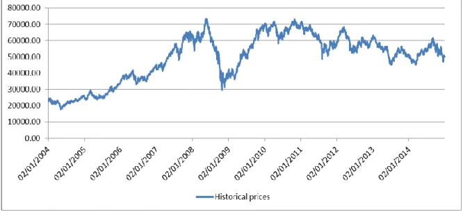
In order to proceed with the analysis of the results, it would be important to observe how the market, represented by the BOVESPA Index, behaved during the period under analysis, i.e. from January 2005 to December 2014. The Brazilian economy has grown during this period, ONU (2015). This growth is reflected on the behavior of its main stock index, as we can observe on the figure below.
FIGURE 1 – Historical prices (2005 – 2014) –BOVESPA Index
Source: BOVESPA (20015).
As observed on the figure, the Index has a steady growth between 2004 and 2008. Then, due to the existence of a high correlation between the performances of the stock markets worldwide with major North American markets and as a consequence of the global financial crisis, the Index suffered a steep declined. However the market’s reaction was very positive, and began its recovery right away, reaching a peak in 2010. From 2010 the
26
Index experienced a period of high volatility, plunged by the slowdown on GDP growth from 4.5% in 2006-10 to 2.1% over 2011-14 and 0.1% in 2014 (World Bank data), but also the devaluation of the Brazilian real against the major currencies and high level of inflation.
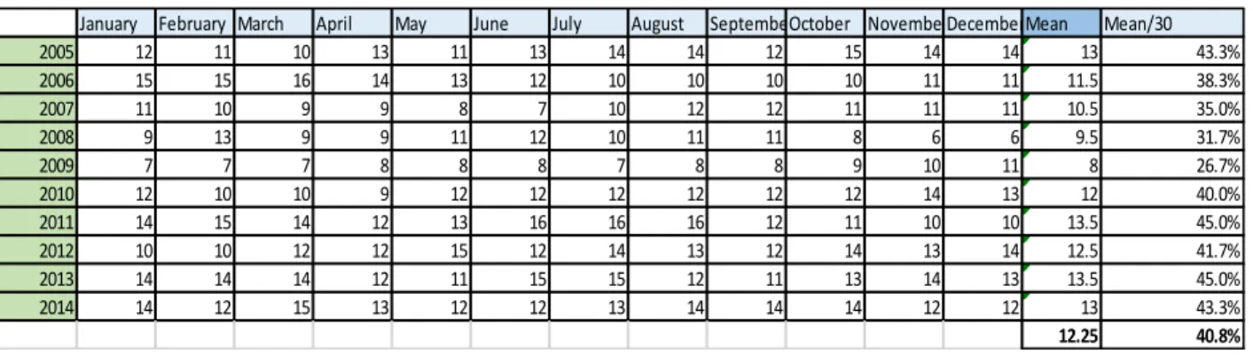
With respect to diversification, the results (tables 3-6) show some interesting outputs. For the mean variance model, the portfolio was composed, on average by 5.75 shares for both time horizon under analysis, representing 19.2% of the shares. We realized that the number of titles drop significantly in 2008, when the mean number of assets was 2, during the big hit the Brazilian equities markets suffered as a consequence of the financial crisis spread worldwide. This evidence contradicts some empirical studies made in the past, Gaumnitz (1969) and Statman (1987), which advocates that the losses are attenuated and the returns increase when the portfolio is diversified, i.e. the number of securities is higher. On the other hand, the minimum variance portfolio was composed, on average, by around 12.25 assets for both “data windows”, so 40.8% of the 30 shares we used on this dissertation. As happened to the mean variance portfolio, the number of assets for the minimum variance model decreased in 2008.
5.2. Hypothesis tests - Results
For both data windows (1 year and 2 years), we tested the hypothesis mentioned above, the results are announced on table 5 and 6. To this end, we resorted to the observation of historical data (10 years) of the BOVESPA Index and to find differences between the use of several models and the impact of these differences on the performance of the investment portfolio in terms of performance and Sharpe ratio. A significance level of 5% was use in
27
these tests. It would also be also useful to understand if the use of different data windows has a statistically significant impact on the study analysis.
Table 1– Hypotheses tests, with 1 year “data window”
Hypotheses Null Hypotheses Alternative Hypotheses tobs p-value Conclusion
HA1 H0:RA=RB H1:RA≠RB 39.09942741 1.11904E-41 Reject H0
HA2 H0:RA=RC H1:RA≠RC 20.91935118 1.11904E-41 Reject H0
HA3 H0:RB=RC H1:RB≠RC 1.318437799 0.189889093 Not Reject H0
HA4 H0:RA=RD H1:RA≠RD 29.58707 1.07335E-56 Reject H0
HA5 H0:RB=RD H1:RB≠RD -1.70539 0.090730206 Not Reject H0
HA6 H0:RC=RD H1:RC≠RD -5.45773 2.67092E-07 Reject H0
HA7 H0:RA=RE H1:RA≠RE 14.75020931 1.23087E-28 Reject H0
HA8 H0:RB=RE H1:RB≠RE -1.01968 0.309951 Not Reject H0
HA9 H0:RC=RE H1:RC≠RE -3.55387 0.000545 Reject H0
HA10 H0:RD=RE H1:RD≠RE -1.173 0.243139 Not Reject H0
HB11 H0:SHA=SHB H1:SHA≠SHB 36.44245083 2.12717E-66 Reject H0 HB12 H0:SHA=SHC H1:SHA≠SHC 23.14278807 7.09495E-46 Reject H0 HB13 H0:SHB=SHC H1:SHB≠SHC -2.384421853 0.018686361 Reject H0 HB14 H0:SHA=SHD H1:SHA≠SHD 26.28866 2.15945E-51 Reject H0 HB15 H0:SHB=SHD H1:SHB≠SHD 0.355748 0.722659033 Not Reject H0 HB16 H0:SHC=SHD H1:SHC≠SHD -0.83642 0.404596263 Not Reject H0 HB17 H0:SHA=SHE H1:SHA≠SHE 21.21921 2.93E-42 Reject H0 HB18 H0:SHB=SHE H1:SHB≠SHE -2.63321 0.009581 Reject H0 HB19 H0:SHC=SHE H1:SHC≠SHE 1.760643 0.080868 Not Reject H0 HB20 H0:SHE=SHD H1:SHR≠SHD -2.63321 0.009581 Reject H0
Regarding the first objective we conclude, based on the results (table 1), there are some statistically significant differences, using a significance level of 5%, in the use of different models presented for both return and Sharpe ratio, except for the minimum variance and naive portfolio, in which we cannot reject the null hypothesis for the returns of both models. For the mean variance adjusted model there are some statistically significant differences, using a significance level of 5%, in relation to the mean variance and minimum variance portfolios, the same is not true with regarding to the Naïve and BOVESPA Index portfolios.
28
For the passive management portfolio which replicates the BOVESPA Index, the results show there are not statistically significant differences in the use of the Index portfolio or the minimum variance based on both return and Sharpe ratio or Naïve portfolios based on the Sharpe ratio.
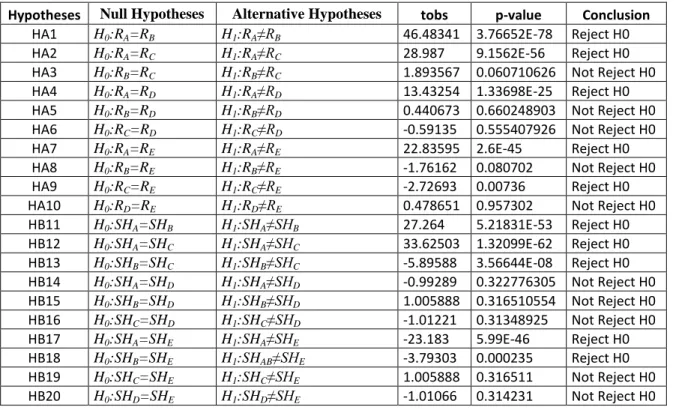
Table 2 – Hypotheses tests, with 2 year “data window”
Hypotheses Null Hypotheses Alternative Hypotheses tobs p-value Conclusion
HA1 H0:RA=RB H1:RA≠RB 46.48341 3.76652E-78 Reject H0
HA2 H0:RA=RC H1:RA≠RC 28.987 9.1562E-56 Reject H0
HA3 H0:RB=RC H1:RB≠RC 1.893567 0.060710626 Not Reject H0
HA4 H0:RA=RD H1:RA≠RD 13.43254 1.33698E-25 Reject H0
HA5 H0:RB=RD H1:RB≠RD 0.440673 0.660248903 Not Reject H0
HA6 H0:RC=RD H1:RC≠RD -0.59135 0.555407926 Not Reject H0
HA7 H0:RA=RE H1:RA≠RE 22.83595 2.6E-45 Reject H0
HA8 H0:RB=RE H1:RB≠RE -1.76162 0.080702 Not Reject H0
HA9 H0:RC=RE H1:RC≠RE -2.72693 0.00736 Reject H0
HA10 H0:RD=RE H1:RD≠RE 0.478651 0.957302 Not Reject H0
HB11 H0:SHA=SHB H1:SHA≠SHB 27.264 5.21831E-53 Reject H0 HB12 H0:SHA=SHC H1:SHA≠SHC 33.62503 1.32099E-62 Reject H0 HB13 H0:SHB=SHC H1:SHB≠SHC -5.89588 3.56644E-08 Reject H0 HB14 H0:SHA=SHD H1:SHA≠SHD -0.99289 0.322776305 Not Reject H0 HB15 H0:SHB=SHD H1:SHB≠SHD 1.005888 0.316510554 Not Reject H0 HB16 H0:SHC=SHD H1:SHC≠SHD -1.01221 0.31348925 Not Reject H0 HB17 H0:SHA=SHE H1:SHA≠SHE -23.183 5.99E-46 Reject H0 HB18 H0:SHB=SHE H1:SHAB≠SHE -3.79303 0.000235 Reject H0 HB19 H0:SHC=SHE H1:SHC≠SHE 1.005888 0.316511 Not Reject H0 HB20 H0:SHD=SHE H1:SHD≠SHE -1.01066 0.314231 Not Reject H0
Through the analysis of table 2, we reach broadly the same conclusions we obtained for the 1 year “data window”.
Therefore, for an investor interested in investing in a portfolio composed by BOVESPA assets, in most of the cases there are statistical evidences saying us that one model is better than the other ones.
29
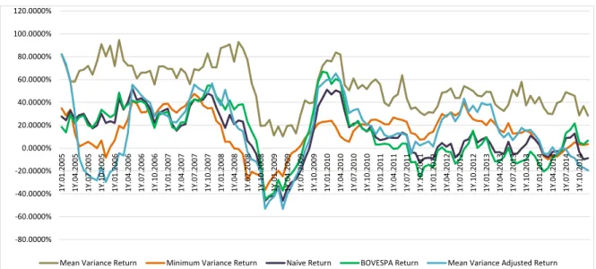
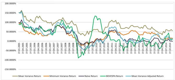
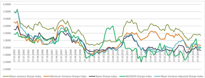
Analyzing the results (figures 2 and 3), we have noticed that the mean-variance model, for “1 year data window” as well as “2 years data window”, has outperformed in terms of returns the other portfolios. Considering Sharpe ratio (chart 4 and 5), the foregoing conclusions are identical. Thus, both Markowitz mean variance portfolio performed better than the other portfolios under analysis.
30
6 Conclusion
6.1. Main Conclusions
The main purpose of this dissertation, was to analyze some models underlying the active and passive portfolio management, by testing some hypothesis regarding the correlation between the mean variance, minimum variance and naive portfolios and what would be its impact on the choice of a certain portfolio. Further to the previous, we aimed to find possible advantages of an actively managed portfolio over a passively managed portfolio.
From the literature review we found De Miguel et. al. (2007) defends the superiority of the passively managed portfolios, while Kritzman et. al. (2010) states that the results from the actively managed portfolios improve when the time horizon increases. By analyzing figures 2-5, we can corroborate Kritzman et. al. (2010) conclusions.
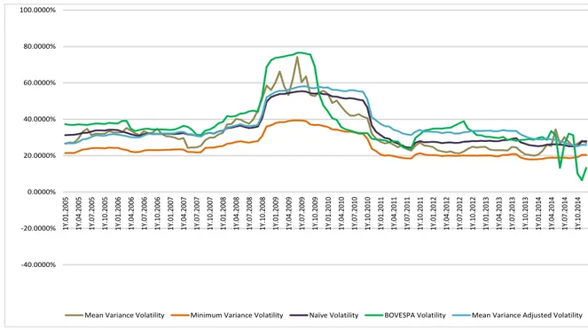
As mentioned in section 5, the main results obtained from the hypotheses tests confirm that there are some significant differences between the different models. Furthermore, the mean variance model had better results in terms of performance (both historical returns and Sharpe ratio) when compared to the other models, which is in line with Kritzman et. al. (2010) and Duchin and Levy (2010). However, the risk associated with this portfolio may be higher, compared to other models used, as the minimum variance and Naïve models, due to its characteristics, as we can confirmed by analyzing figures 6 and 7.
Concerning the portfolio which the aim is to track the index performance, the main conclusion is that the Index underperformed the mean variance portfolio. However we cannot perform any analysis in relation to the minimum variance and Naïve portfolio, as the
31
hypotheses tests revealed no significance statistical difference between the BOVESPA Index portfolio and the remaining model based portfolios.
In theory, strategies related with the minimum-variance portfolio aim to obtain a highest performance using the risk management during periods of financial crisis. Nevertheless, we verified that during the financial crisis (2008-2009), the mean variance model performed better than the minimum variance portfolio, as well.
In summary, based on the results, we can affirm that the mean variance portfolio should be chosen, as performed better both in terms of returns and , especially, in terms of Sharpe ratio when compared with the other two portfolios.
6.2. Limitations and Further Research
This study has some limitation concerning the time horizon. The use history of the securities prices of only 10 years does not allow us a deeper and more consistent analysis in comparison with other studies that have a longer historical record. We could have used other shorter time periods as well, to test whether we find different results.
Furthermore if we had used others optimization models, beside the mean variance model, the conclusions could be different. As it could be used other measure of performance than Sharpe index, such as indices or Treynor Jensen.
Regarding future research, it would be interesting to apply this study not only to stock portfolios, but also to bonds, real estate or derivatives, and to include other South America markets, as well, as the MERVAL (Argentina) or the BCS (Chile).
32
Finally one could extend the time horizon of the study, as well, making a thorough analysis of the events that may contribute to the existence of large fluctuations in returns and risk of securities.
33
7 References
1. Bawa V. (1976), “Admissible portfolios for all individuals”, Journal of Finance, Vol. 31, No 4, pp. 1169-1181.
2. Bodie, Z., Kane, A. and Markus, A. (2009), “Investments”, 8th edition, The MacGraw Hill Companies.
3. Chow, G., Jacquier, E., Kritzman, M. and Lowry, K. (1999), “Optimal Portfolio In Good Times and Bad”, Financial Analysis Journal, Vol. 55, No. 3, pp. 65-73.
4. Clarke, R., de Silva, H. and Thorley, S. (2006), “Minimum-Variance Portfolio in the U.S. Equity Market”, The Journal of Portfolio Management, Vol. 33, No. 1, pp. 10-24. 5. Cvitanic, J., Lazrak, A. and Wang, T. (2008), “Implications of the Sharpe Ratio as a performance measure in multi-period settings”, Journal of Economic Dynamics & Control, Vol. 32, No. 5, pp. 1622-1649.
6. De Miguel, V., Garlappi, L. and Uppal, R., (2007), “Optimal Versus Naïve Diversification: How Inefficient ir the 1/N Portfolio Strategy?” Review of Financial Studies, Vol. 22, No. 5, pp. 1915-1953.
7. Duchin, R. and Levy, H. (2009),”Markowitz Versus the Talmudic Portfolio Diversification Strategies”, The Journal of Portfolio Management, Vol. 35, No. 2, pp. 71-74.
8. Elton, E., Grubber, M., Brown, S. and Goetzmann, W. (2011), “Modern Portfolio Theory and Investment Analysis”, Eighth Edition, John Willey & Sons, New York.
9. Evans, J., and Archer, S. (1968), “Diversification and the Reduction of Dispersion”. Journal of Finance, 23(5), 761-767.
10. Fischer, Hans (2010), “A History of the Central Limit Theorem: From Classical to Modern Probability”, First Edition, Springer, New York.
11. Gaumnitz, J. E. (1969), “Risk, return and equilibrium”, unpublished paper, Graduate School of Business, The University of Chicago, March.
12. Grauer, R. R. September (1986). “Normality, solvency and portfolio choice”. Journal of Financial and Quantitative Analysis, 21:265-278.
13. Horasanli, M. and Fidan, N. (2007), “Portfolio Selection by Using Time Varying Covariance Matrices”, Journal of Economics & Social Research, Vol.9, No. 2, pp. 1-22.
34
14. Jensen, M. J. (1968), “The performance of mutual funds in the period 1945-1964”, Journal of Finance, Vol. 23, No. 2, pp. 389-416.
15. Kwan, C. C. Y. (2001), “Portfolio analysis using spreadsheets tools”, Journal of Applied Finance, Vol. 11, pp. 70-81.
16. Kritzman, M. Page, S. Turkington, D. (2010), “In Defense of Optimization: The Fallacy on 1/N”, Financial Analysts Journal, Vol. 66, No. 2, pp. 1-9.
17. Levy, H., and Markowitz, H. (1979), “Approximating Expected Utility by a Function of Mean and Variance,” American Economic Review, 69, 308–317.
18. Lo, A. (2002), “The statistics of Sharpe ratios”, Financial Analysts Journal, CFA Institute.
19. Markowitz, H. (1952), “Portfolio selection”, Journal of Finance, Vol. 7, No. 1, pp. 77-91.
20. Markowitz, H. (1959), ‘’Portfolio selection: efficient diversification of investment”, New York, John Wiley and Sons, Inc.
22. Markowitz, H. (2012), “Mean-variance approximation to expected utility”, European Journal of Operational Research, 234, pp. 346-355.
23. Pogue, G.A. (1970), “An extension of the Markowitz portfolio selection model to include variable transaction costs, short sales, leverage policies and taxes”, The Journal of Finance, Vol. 25, No. 5, pp. 1005-1027.
24. Pulley, L.B. 1983. “Mean-Variance Approximations to Expected Logarithmic Utility”, Operations Research, 3 1: 685-696.
25. Rubinstein, M. (2002), ‘’Markowitz’s “Portfolio Selection”: A Fifty-Year Retrospective’’, The Journal of Finance, Vol. 57, No. 3, pp. 1041-1045.
26. Scholz,H. and Wilkens, M. (2005), “Investor-specific performance measurement: a justification of Sharpe Ration and Treynor Ratio”, The International Journal of Finance, Vol. 17, No. 4, pp. 3671-3691.
27. Sharpe, W. F. (1966), “Mutual fund performance”, Journal of Business, Vol. 39, No.1, pp. 49-58.
28. Simaan, Youriff (1993), “Portfolio Selection and Asset Pricing—Three-Parameter
35
29. Statman, M. (1987), “How many stocks make a diversified portfolio?”, Journal of Finance and Quantitive Analysis, Vol. 22, No. 3, pp. 353-363.
30. Organization of United Nations, United Nations Statistics Division [Online], available
36
8 Appendix
Table 3 – Number of assets invested – mean variance portfolio for “1 year data window”.
Table 4 – Number of assets invested – mean variance portfolio for “2 year data window”.
Table 5 – Number of assets invested – minimum variance portfolio for “1 year data window”.
January February March April May June July August SeptemberOctober NovemberDecemberMean Mean/30 2005 3 3 4 4 5 3 3 3 3 6 4 5 3.5 11.7% 2006 5 7 7 7 10 7 9 6 5 4 4 6 6.5 21.7% 2007 6 5 3 6 5 6 5 7 8 6 6 5 6 20.0% 2008 2 2 3 3 2 3 2 2 2 2 1 1 2 6.7% 2009 1 2 1 2 1 1 1 2 3 3 7 8 2 6.7% 2010 6 6 6 9 8 5 5 6 5 5 7 5 6 20.0% 2011 6 7 7 7 7 7 7 7 4 3 5 4 7 23.3% 2012 5 6 5 6 5 4 5 6 6 6 5 7 5.5 18.3% 2013 7 6 7 7 6 9 6 6 4 6 7 7 6.5 21.7% 2014 4 3 3 2 4 2 3 5 5 3 2 4 3 10.0% 5.75 19.2%
January February March April May June July August SeptemberOctober NovemberDecemberMean Mean/30 2005 8 6 9 8 10 9 9 10 8 8 8 8 8 26.7% 2006 8 8 8 8 8 6 7 7 6 9 10 8 8 26.7% 2007 7 9 10 9 9 8 8 9 5 6 6 6 8 26.7% 2008 7 5 6 4 3 5 5 5 6 5 3 3 5 16.7% 2009 3 2 4 5 5 3 3 2 2 2 2 2 2.5 8.3% 2010 5 6 4 4 4 3 3 3 4 5 8 6 4 13.3% 2011 7 7 8 7 7 6 9 9 6 5 5 5 7 23.3% 2012 4 5 6 7 7 6 6 6 6 5 4 5 6 20.0% 2013 5 5 5 6 6 6 5 4 5 6 7 8 5.5 18.3% 2014 8 6 4 5 2 7 4 5 9 6 5 6 5.5 18.3% 5.75 19.2%
January February March April May June July August SeptemberOctober NovemberDecemberMean Mean/30
2005 12 11 10 13 11 13 14 14 12 15 14 14 13 43.3% 2006 15 15 16 14 13 12 10 10 10 10 11 11 11.5 38.3% 2007 11 10 9 9 8 7 10 12 12 11 11 11 10.5 35.0% 2008 9 13 9 9 11 12 10 11 11 8 6 6 9.5 31.7% 2009 7 7 7 8 8 8 7 8 8 9 10 11 8 26.7% 2010 12 10 10 9 12 12 12 12 12 12 14 13 12 40.0% 2011 14 15 14 12 13 16 16 16 12 11 10 10 13.5 45.0% 2012 10 10 12 12 15 12 14 13 12 14 13 14 12.5 41.7% 2013 14 14 14 12 11 15 15 12 11 13 14 13 13.5 45.0% 2014 14 12 15 13 12 12 13 14 14 14 12 12 13 43.3% 12.25 40.8%
37
Table 6 – Number of assets invested – minimum variance portfolio for “2 year data window”.
Figure 2 – Returns – Mean Variance, Minimum Variance, Mean Variance Adjusted, Naive and BOVESPA Index portfolios (1 year “data windows”)
January February March April May June July August SeptemberOctober NovemberDecemberMean Mean/30
2005 12 13 12 13 14 14 13 13 13 13 13 13 13 43.3% 2006 13 12 12 12 12 12 11 12 11 12 12 11 12 40.0% 2007 11 11 11 11 11 10 11 10 10 12 11 10 11 36.7% 2008 10 11 11 11 11 11 12 11 11 10 7 7 11 36.7% 2009 8 8 8 8 8 8 8 8 8 8 8 8 8 26.7% 2010 8 8 8 8 8 8 8 8 8 10 9 11 8 26.7% 2011 10 11 12 12 14 13 14 15 13 13 13 13 13 43.3% 2012 13 12 13 15 15 13 14 15 13 13 14 13 13 43.3% 2013 13 14 14 15 14 16 14 13 15 12 14 12 14 46.7% 2014 12 11 11 11 11 13 14 14 13 14 12 13 12.5 41.7% 12.25 40.8% -80.0000% -60.0000% -40.0000% -20.0000% 0.0000% 20.0000% 40.0000% 60.0000% 80.0000% 100.0000% 120.0000% 1Y .01.2005 1Y .04.2005 1Y .07.2005 1Y .10.2005 1Y .01.2006 1Y .04.2006 1Y .07.2006 1Y .10.2006 1Y .01.2007 1Y .04.2007 1Y .07.2007 1Y .10.2007 1Y .01 .200 8 1Y .04.2008 1Y .07.2008 1Y .10.2008 1Y .01.2009 1Y .04.2009 1Y .07.2009 1Y .10.2009 1Y .01.2010 1Y .04.2010 1Y .07.2010 1Y .10.2010 1Y .01.2011 1Y .04.2011 1Y .07.2011 1Y .10.2011 1Y .01 .201 2 1Y .04.2012 1Y .07.2012 1Y .10.2012 1Y .01.2013 1Y .04.2013 1Y .07.2013 1Y .10.2013 1Y .01.2014 1Y .04.2014 1Y .07.2014 1Y .10.2014
38
Figure 3 – Returns – Mean Variance, Minimum Variance, Mean Variance Adjusted, Naive and BOVESPA Index portfolios (2 years “data windows”)
Figure 4 – Sharpe Index – Mean Variance, Minimum Variance, Mean Variance Adjusted, Naive and BOVESPA Index portfolios (1 years “data windows”)
-150.0000% -100.0000% -50.0000% 0.0000% 50.0000% 100.0000% 150.0000% 200.0000% 1Y .01.2005 1Y .04.2005 1Y .07.2005 1Y .10.2005 1Y .01.2006 1Y .04.2006 1Y .07.2006 1Y .10.2006 1Y .01.2007 1Y .04.2007 1Y .07.2007 1Y .10.2007 1Y .01 .200 8 1Y .04.2008 1Y .07.2008 1Y .10.2008 1Y .01.2009 1Y .04.2009 1Y .07.2009 1Y .10.2009 1Y .01.2010 1Y .04.2010 1Y .07.2010 1Y .10.2010 1Y .01.2011 1Y .04.2011 1Y .07.2011 1Y .10.2011 1Y .01 .201 2 1Y .04.2012 1Y .07.2012 1Y .10.2012 1Y .01.2013 1Y .04.2013 1Y .07.2013 1Y .10.2013 1Y .01.2014 1Y .04.2014 1Y .07.2014 1Y .10.2014
Mean Variance Return Minimum Variance Return Naïve Return BOVESPA Return Mean Variance Adjusted Return
-3.0000 -2.0000 -1.0000 0.0000 1.0000 2.0000 3.0000 4.0000 1Y .01.2005 1Y .04.2005 1Y .07.2005 1Y .10.2005 1Y .01.2006 1Y .04.2006 1Y .07.2006 1Y .10.2006 1Y .01.2007 1Y .04.2007 1Y .07.2007 1Y .10.2007 1Y .01.2008 1Y .04.2008 1Y .07.2008 1Y .10.2008 1Y .01.2009 1Y .04.2009 1Y .07.2009 1Y .10.2009 1Y .01.2010 1Y .04.2010 1Y .07.2010 1Y .10.2010 1Y .01.2011 1Y .04.2011 1Y .07.2011 1Y .10.2011 1Y .01.2012 1Y .04.2012 1Y .07.2012 1Y .10.2012 1Y .01.2013 1Y .04.2013 1Y .07.2013 1Y .10.2013 1Y .01.2014 1Y .04.2014 1Y .07.2014 1Y .10.2014
39
Figure 5 - Sharpe Index – Mean Variance, Minimum Variance, Mean Variance Adjusted, Naive and BOVESPA Index portfolios (2 years “data windows”)
Figure 6 - Volatility – Mean Variance, Minimum Variance, Mean Variance Adjusted, Naive and BOVESPA Index portfolios (1 years “data windows”)
-3.0000 -2.0000 -1.0000 0.0000 1.0000 2.0000 3.0000 4.0000 5.0000 6.0000 1Y .01 .2 00 5 1Y .04 .2 00 5 1Y .07 .2 00 5 1Y .10 .2 00 5 1Y .01 .2 00 6 1Y .04 .2 00 6 1Y .07 .2 00 6 1Y .10.2 006 1Y .01 .2 00 7 1Y .04 .2 00 7 1Y .07 .2 00 7 1Y .10 .2 00 7 1Y .01 .2 00 8 1Y .04 .2 00 8 1Y .07 .2 00 8 1Y .10 .2 00 8 1Y .01 .2 00 9 1Y .04 .2 00 9 1Y .07 .2 00 9 1Y .10 .2 00 9 1Y .01 .2 01 0 1Y .04.2 010 1Y .07 .2 01 0 1Y .10 .2 01 0 1Y .01 .2 01 1 1Y .04 .2 01 1 1Y .07 .2 01 1 1Y .10 .2 01 1 1Y .01 .2 01 2 1Y .04 .2 01 2 1Y .07 .2 01 2 1Y .10 .2 01 2 1Y .01 .2 01 3 1Y .04 .2 01 3 1Y .07 .2 01 3 1Y .10 .2 01 3 1Y .01 .2 01 4 1Y .04 .2 01 4 1Y .07 .2 01 4 1Y .10 .2 01 4
Mean variance Sharpe Index Minimum Variance Sharpe Index Naïve Sharpe Index BOVESPA Sharpe Index Mean Variance Adjusted Sharpe Index
10.0000% 20.0000% 30.0000% 40.0000% 50.0000% 60.0000% 70.0000% 80.0000% 1Y .01.2005 1Y .04.2005 1Y .07.2005 1Y .10.2005 1Y .01.2006 1Y .04.2006 1Y .07.2006 1Y .10.2006 1Y .01.2007 1Y .04.2007 1Y .07.2007 1Y .10.2007 1Y .01.2008 1Y .04.2008 1Y .07.2008 1Y .10.2008 1Y .01.2009 1Y .04.2009 1Y .07.2009 1Y .10.2009 1Y .01.2010 1Y .04.2010 1Y .07.2010 1Y .10.2010 1Y .01.2011 1Y .04.2011 1Y .07.2011 1Y .10.2011 1Y .01.2012 1Y .04.2012 1Y .07.2012 1Y .10.2012 1Y .01.2013 1Y .04.2013 1Y .07.2013 1Y .10.2013 1Y .01.2014 1Y .04.2014 1Y .07.2014 1Y .10.2014
40
Figure 7 - Volatility – Mean Variance, Minimum Variance, Mean Variance Adjusted, Naive and BOVESPA Index portfolios (2 year “data windows”)
-40.0000% -20.0000% 0.0000% 20.0000% 40.0000% 60.0000% 80.0000% 100.0000% 1Y .01.2005 1Y .04.2005 1Y .07.2005 1Y .10.2005 1Y .01.2006 1Y .04.2006 1Y .07.2006 1Y .10.2006 1Y .01.2007 1Y .04.2007 1Y .07.2007 1Y .10.2007 1Y .01.2008 1Y .04.2008 1Y .07.2008 1Y .10.2008 1Y .01.2009 1Y .04.2009 1Y .07.2009 1Y .10.2009 1Y .01.2010 1Y .04.2010 1Y .07.2010 1Y .10.2010 1Y .01.2011 1Y .04.2011 1Y .07.2011 1Y .10.2011 1Y .01.2012 1Y .04.2012 1Y .07.2012 1Y .10.2012 1Y .01.2013 1Y .04.2013 1Y .07.2013 1Y .10.2013 1Y .01.2014 1Y .04.2014 1Y .07.2014 1Y .10.2014