MASTER in FINANCE MASTER’S FINAL WORK

MASTER in

FINANCE

MASTER’S FINAL WORK

DISSERTATION

Robust Mean Variance

João Nuno Martins Cardoso

MASTER in

FINANCE

MASTER’S FINAL WORK

DISSERTATION

ROBUST MEAN VARIANCE

João Nuno Martins Cardoso

Supervisor:

Raquel Medeiros Gaspar

Abstract

This empirical study’s objective is to evaluate the impact of robust estimation on mean variance portfolios. This was accomplished by doing a simulation on the behavior of 15

SP500 stocks. This simulation includes two scenarios: One with normally distributed

samples and another with contaminated non-normal samples. Each scenario includes

200 resamples. The performance of maximum likelihood (classical) estimated

portfolios and robustly estimated portfolios are compared, resulting in some

conclusions: On normally distributed samples, robust portfolios are marginally less

efficient than classical portfolios. However, on non-normal samples, robust portfolios

present a much higher performance than classical portfolios. This increase in

performance is positively correlated with the level of contamination present on the

sample. In summary, assuming that financial returns do not present a normal

distribution, we can state that robust estimators result in more stable mean variance

Resumo

Este estudo empírico tem como objectivo avaliar o impacto da estimação robusta nos

portefólios de média variância. Isto foi conseguido fazendo uma simulação do

comportamento de 15 acções do SP500. Esta simulação inclui dois cenários: um com

amostras que seguem uma distribuição normal e outro com amostras contaminadas

não normais. Cada cenário inclui 200 reamostragens. O performance dos portefólios

estimados usando a máxima verosimilhança (clássicos) e dos portefólios estimados de

forma robusta são comparados, resultando em algumas conclusões: Em amostras

normais, portefólios robustos são marginalmente menos eficientes que os portefólios

clássicos. Contudo, em amostras não normais, os portefólios robustos apresentam um

performance muito superior que os portefólios clássicos. Este acréscimo de

performance está positivamente correlacionado com o nível de contaminação da

amostra. Em suma, assumindo que os retornos financeiros têm uma distribuição não

normal, podemos afirmar que os estimadores robustos resultam em portefólios de

Table of Contents

Table of Contents...iv

List of Tables ... v

List of Figures ... v

1. Introduction ... 1

2. Literature Review ... 3

2.1 MVT Applications & Shortcomings ... 3

2.2 Estimation Risk ... 4

2.3 Mean Variance Theory extensions ... 5

2.4 Robust Statistics ... 7

3. Methodology ... 10

3.1 Data ... 11

3.2 Monte Carlo Simulation ... 13

3.2.1 Control scenario ... 13

3.2.2 Contamination scenario ... 15

3.3 Robust estimator ... 16

3.4 Portfolio creation process ... 17

4. Results ... 19

4.1 Control scenario ... 19

4.1.1 Tangent Portfolios ... 21

4.1.2 Average and naive portfolio ... 25

4.2 Contamination Scenario ... 27

4.2.1 Tangent portfolios ... 28

4.2.2 Average and naive portfolio ... 31

5. Conclusion ... 34

List of Tables

Table I - Stock description………...………...………...……..11

Table II - Control Scenario descriptive statistics………...………...………....……..14

Table III - Contamination Scenario descriptive statistics……….16

Table IV - Sharpe Ratio of tangent portfolios on the true efficient frontier……..………30

Table V - Sharpe Ratio of average portfolios………..33

List of Figures

Figure 2 - Tangent portfolios ………...……….………21

Figure 3 - Classical risk/return scatter ……….23

Figure 4 - Robust risk/return scatter ………..……….23 Figure 5 - Sharpe Ratio distribution……….……….….……..24

Figure 6 - Dispersion of tangent portfolios’ allocation……….……….………..25/26 Figure 7 - Average and Naive Portfolios.………..………...….26

Figure 8 - Dispersion of estimated tangent portfolios (5% contamination 2.5 magnitude)………28

Figure 9 - Dispersion of estimated tangent portfolios (5% contamination 5 magnitude)……...28

Figure 10 - Dispersion of estimated tangent portfolios (5% contamination 10 magnitude)…....29

1. Introduction

The purpose of this paper is to study the effect of estimation risk on the stability of

portfolios resulting from Mean Variance Theory (MVT), developed by the work of

Markowitz (1952, 1959). It is focused on problems on practical applications of MVT,

contrasting with the fact that in theory it produces optimal results and is the backbone

of modern portfolio theory. Nonetheless, its translation into real life is not perfect, as

the composition of the optimal portfolio1 is unstable over time and too sensitive to ill

estimations of parameters, resulting in it being unconsidered by many portfolio

managers, topic that was explored by Michaud (1989). How can a model like this be

considered the answer for portfolio allocation problems and then result in less than

efficient portfolios on its practical applications? See Jobson and Korkie (1981).

To answer this question, first we should start by looking in to MVT and understand

how it works. This theory takes a basket of n securities and allocates them in order to

maximize expected returns for each possible risk level, on a certain investment period.

Resulting in a curve in risk/expected return plan, representing the set of efficient

portfolios, called efficient frontier. One of the advantages of MVT is its simplicity, mainly because it relies on two inputs:, a vector composed with n securities’

expected returns and , a n n* variance-covariance matrix of the respective expected returns. In MVT the optimization problem is treated as a deterministic

problem, i.e. it is assumed that both  and  which are be applied to the investment period are known with certainty. In real life, of course, these two inputs have to be

estimated, and so they are subject to estimation error. The assumption that one knows for sure the future expected returns and future variance-covariance of expected

returns of the different assets is difficult to stand. In practice, investors have to

forecast those inputs, which inevitably results in estimation error. Estimation risk is

therefore the main source of risk in MVT. As Fabozzi et al (2014) defended, the

irrational relation between inputs and outputs and the great sensitivity of the portfolio

On this study, several questions have to be answered. First, why does MVT produce

sub-optimal portfolios in practice? How can robust estimators improve the stability of

the resulting portfolios? How robust estimators perform in comparison with classical

Maximum Likelihood estimators under different scenarios? And finally, how different

degrees of parameter deviation affect the stability of the final output of MVT?

We start by positioning this study with respect to what has already been done on this

subject on chapter 2, showing several studies about MVT risk mitigation, optimization

of the estimation process and portfolio optimization procedures. Additionally, in this

chapter we demonstrate how this work differs from those past studies. Then on

chapters 3 we present the methodology used. On chapter 4 a simulation study of 15

Standard and Poor’s stocks is presented, where the performance of classical Maximum Likelihood estimators and robust estimators is compared. On chapter 5 some

2. Literature Review

Mean Variance Theory developed by Markowitz (1952, 1959) has been the basis of

modern portfolio theory. Before him, the focus of investment selection was on

evaluating securities individually in order to decide which securities yielded the higher

returns. Not taking in account the risk associated with those securities. After

Markowitz the focus changed to diversification and the impact of each security on a

portfolio’s total risk-return.

This literature review starts by taking a look at the main breakthroughs that MVT

allowed, as well as the limitations of this theory on section 2.1. Subsequently, on

section 2.2, are presented the major developments related with estimation risk, which

is a very important topic through this paper. On the next section (2.3), are presented

some important improvements and alternatives to classical MVT. To conclude, section

2.4 presents a review on robust statistics.

2.1 MVT Applications & Shortcomings

Since its creation MVT has been widely used by researchers and practitioners. In the

academia it laid the ground for several equilibrium models, like CAPM, produced

through the work of Lintner (1965), Mossin (1966) and Sharpe (1966). It was also

important in defining and understanding the difference between systematic and

diversifiable risk. For practitioners it is important in many portfolio management

applications. However, despite the simplicity of the model created by Markowitz, the

powerful optimization theory supporting it and the existence of software able to easily

solve the optimization problem, it is still disregarded in practice due to its poor ability

to adapt to estimated inputs and due to the sensibility of optimal portfolios to small

changes in inputs, see Michaud (1989). If we divide MVT in two parts, first we have the

process of computing the inputs and secondly the optimization of those same inputs in

results, whereas on the second part, the process is flawless. Though, the second part

only results in solid portfolio allocations if the first part produced exact inputs, which

most of the times is not possible.

MVT is based on the assumption that the vector of expected returns

 

 

historical prices of those same securities. Therefore, the actual inputs of MVT are ˆ

and ˆ , which have some associated estimation error. This is a shortcoming of MVT,

which does not take in account the fact that inputs were estimated, and include

estimation error, treating them as the unbiased parameters. This is commonly referred

to as “certainty equivalence”, as those estimated parameters are considered equivalent to the known parameters through the whole optimization process.

2.2 Estimation Risk

Estimation risk is a fundamental factor for the inefficiency of Mean Variance efficient

portfolios. Merton (1980) has shown that expected returns are extremely sensitive to

estimation error, variance is slightly sensitive and covariance is the less sensitive of the

three. We also know that even small changes in input parameters may result in large

changes in the optimal portfolio composition, Chopra (1993). Additionally, Chopra and

Ziemba (1993) concluded that “errors in means are approximately 10 times as important as errors in variances and covariances considered together”. So, considering that investors have limited resources, they should focus their resources on finding the

best possible estimates of expected returns, as this parameter is the one which most

influences the quality of the estimated tangent portfolio.

Jobson and Korkie (1981) made a simulation study where they estimated the expected

return and risk of 20 securities from a simulated dataset of 60 monthly returns. The

estimated tangent portfolio had a Sharpe ratio of 0.08, compared with the Sharpe ratio

weighted portfolio of those same 20 securities, concluding that MV efficient portfolios

can even be dominated by naive portfolios of the same assets due to the effect of

estimation error.

Taking a different perspective, Michaud (1989) introduced the concept of “estimation

error maximizers”, defending that MVT behaves as a maximizer of estimation risk. Securities that have its expected return overestimated (underestimated), its standard

deviation underestimated (overestimated) or its covariance underestimated

(overestimated) will be overweighted (underweighted) on the resulting portfolio. This

acts as proof of the ill effect of estimation risk on the output of the optimal portfolio composition.

Best and Grauer (1991) made a computational simulation on the behavior of portfolios

of different sizes and reached the conclusion that when changing the expected return

of one asset, the composition, expected return and risk of the optimal portfolio

changed drastically. Although when a non-negativity constraint was present the

portfolio composition was still very sensitive to changes in one security expected

return, but the expected return and risk of the portfolio tended to remain almost

constant.

What all of those studies show is that estimation risk has a big impact on portfolio

allocation problems. More than changing the portfolio composition, it may also affect

deeply the portfolio’s expected return and risk. Hence, estimation risk has to be

mitigated as much as possible, something that researchers have been doing but is still

a work in progress, like we can see on the next section.

2.3 Mean Variance Theory extensions

The inability of MVT to cope with estimated parameters and the fact that it did not

acknowledge the existence of estimation error on its inputs has been criticized by

several authors like Barry (1974), Bawa and Klein (1979), Brown (1976).

According to Stein (1956) for an estimator to be admissible it must dominate all other

inadmissibility of sample means as estimators of expected returns. Based on this

development Jobson et al(1979) proposed a James-Stein estimator to improve the

efficiency of MVT, this estimator was put to the test on Jobson and Korkie (1981) and

consists on a Bayesian estimator which shrinks the individual means of each security to

a global mean, in a way that, the greater the volatility of each security, the greater the

shrinkage, Jorion (1986) proposed a similar estimator, but shrinking the expected

return estimates towards the minimum variance portfolio.

Black Litterman (1991) introduced a market based shrinkage approach which combines

equilibrium expected returns based on the weighted average market return from

CAPM with investor’s views on each asset or group of assets and with the investor’s

degree of confidence on each forecast. An important assumption of this model is that

the expected return of a security should be consistent with the market equilibrium

unless the investor has a particular view on that security. Therefore, an investor

without any views (unconstrained) should hold the market portfolio. Another possible

way to correct the ill effect of estimation error is to increase the risk aversion

parameter. That is exactly what Horst, Roon and Werker (2002) did, developing a risk

aversion correction to take estimation risk into account when estimating mean

variance tangent portfolios, this new risk aversion is higher than the standard one and

the increase depends on the sample size, number of securities on the portfolio and on

the curvature of the mean variance frontier. This way, considering that the estimated

efficient frontier is an overestimation of the true efficient frontier due to the error maximization effect, increasing the risk aversion parameter nullifies some of that

overestimation.

On 1998 Michaud presented a resampling methodology to mitigate estimation risk on

a mean variance framework. Through statistical resampling, several risk/return

estimates are created, from those estimates, tangent portfolios are created and by

averaging the weights of those tangent portfolios an investor can reach a solid

estimate of an optimal portfolio.

On the late 90’s, a method that considers estimation error as part of the optimization

introduced by El Ghaoui and Lebret (1997) and Ben-Tal and Nemirovski (1998). It

consists on finding a solution that is satisfactory to most possible realizations of the

uncertain parameters





the set, the more uncertain is the parameter (higher chance of estimation error) and

more robust is the solution. The problem is then solved by finding the portfolio that

maximizes utility on the worst-case scenario, from the possible values of the

uncertainty set. See for instance: Lobo and Boyd (2000) and Goldfarb and Iyengar

(2003). Even using any of these enhancements of MVT, and due to the stochastic

behavior of the asset return process, estimation error will always exist, even if it is

lower than the vanilla MVT.

2.4 Robust Statistics

What would be preferred by an investor: (i) make a solid estimation of expected

returns and covariances of a set of securities or (ii) make an estimation that considers

the infinitesimal probability of a sudden market crisis but isn’t as reliable as the first

one on a non-crisis scenario? Should investors give the same importance to extreme

returns as they do to more common returns? This results in a problem of statistical

robustness. Robust statistics, developed by Huber (1964) and Hampel (1968), consists

on procedures to deal with situations where the underlying distribution deviates

slightly from the assumed model, see Huber and Ronchetti (1981). On MVT, extreme

observations with a very few chance of happening have a great effect on the estimated

input parameters.

It is then important to clarify two concepts: efficiency and breakdown of estimators.

Efficiency is the capability of an estimator to yield close to optimal estimates, therefore

to minimize estimation errors. Breakdown is the amount of outlying observations that

an estimator can withstand before it produces unstable results, see Huber and

Ronchetti (1981). Usually, the more efficient an estimator is, the lower is its

breakdown point, and vice versa. For example, if we compare the classical mean and

as it tends to produce closer to optimal estimates. However, if we multiply the highest

observation on a given sample by one million, the mean of that sample would be

heavily biased by it, whereas its median would remain the same. Consequently robust

estimators, the ones with a considerable higher breakdown point have an implied loss

of efficiency associated with gains in stability, Huber and Ronchetti (1981).

An estimator is considered robust if it can withstand extreme observations and still

yield stable estimations. Classical estimators are known to result in dire results on the

presence of those observations as its breakdown point is or is close to zero. One way

to assess if an estimator is robust is to study its Influence Function. This function

resulted from the work of Hampel (1968, 1974) as it “allows us to assess the relative

influence of individual observations towards the value of an estimate or test statistic” and therefore “allows an immediate and simple heuristic assessment of the asymptotic

properties of an estimate” Huber and Ronchetti (1981). Furthermore, Hampel (1986) has stated that the only necessary condition for an estimator to be robust is for it to

have a bounded influence function, consequently the only condition necessary for

MVT to be robust is to have its parameters estimated through robust estimators with

bounded influence functions.

On this study we see how estimation error and the inclusion of “noise” on the sample, affect the quality of the estimated parameters. Studying the effect of different

magnitudes and frequencies of sample contamination and how robust estimators

perform in comparison to classical estimators on all those different scenarios. To do

this, we use a resampling method similar to the one developed by Michaud (1998).

Though, on our case, two different estimates are applied to each sample, one classical

and one robust and different kind of samples are used. In addition, we are able to see

3. Methodology

In order to compare the performance of tangent portfolios resulting from classically

and robustly estimated efficient frontiers, we simulate the returns of a set of stocks

through a resampling process. This is repeated to several different scenarios. On each

scenario, both types of estimations are applied to all samples, resulting in a number of

different estimated parameters. From there, MVT is applied on each different

scenario, for both estimation types and for all resamples, resulting in several estimated

tangent portfolios which are the main tools to study the advantages and disadvantages

of each estimator.

On this chapter this methodology is explained in detail. On section 3.1 we start by

presenting the data which served as base for this empirical study. Section 3.2 is where

the simulation methodology is presented, being then divided in subsection 3.2.1 and

3.2.2. On subsection 3.2.1 the control scenario, the one which does not contain any

contamination, is explained. In opposition, subsection 3.2.2 describes the different

contamination scenarios, and how the contamination process occurred. Section 3.3

shows in more detail the robust estimator which is used on this study. And finally

3.1 Data

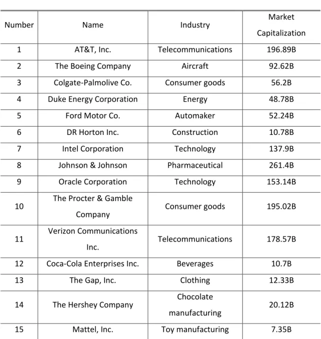
A set of 15 Standard & Poor’s stocks are the objects of the simulation, all of them having been in the index for more than 20 years. This set of stocks encompasses

companies from different industries and sizes.

Table I – Stock description

Number Name Industry

Market

Capitalization

1 AT&T, Inc. Telecommunications 196.89B

2 The Boeing Company Aircraft 92.62B

3 Colgate-Palmolive Co. Consumer goods 56.2B

4 Duke Energy Corporation Energy 48.78B

5 Ford Motor Co. Automaker 52.24B

6 DR Horton Inc. Construction 10.78B

7 Intel Corporation Technology 137.9B

8 Johnson & Johnson Pharmaceutical 261.4B

9 Oracle Corporation Technology 153.14B

10

The Procter & Gamble

Company Consumer goods 195.02B

11

Verizon Communications

Inc. Telecommunications 178.57B

12 Coca-Cola Enterprises Inc. Beverages 10.7B

13 The Gap, Inc. Clothing 12.33B

14 The Hershey Company

Chocolate

manufacturing 20.12B

15 Mattel, Inc. Toy manufacturing 7.35B

Since we want to mitigate idiosyncratic risk as much as possible, 15 stocks should be

enough to generate diversified portfolios. See, for instance, the comments about a

diversified portfolio of Reilly (1985): “In terms of overdiversification, several studies have shown that it is possible to derive most of the benefits of diversification with a portfolio consisting of from 12 to 18 stocks. To be adequately diversified does not

require 200 stocks in a portfolio” pp.(213).

Monthly observations from April 1995 to March 2015 were extracted for each stock.

To minimize estimation error as much as possible, a sample of 240 monthly returns

was used for each stock, given that according to Jobson and Korkie (1981) 60 to 100

monthly returns are not enough to eliminate estimation error. The authors also note

that a sample of at least 200 monthly returns would be needed in order to minimize

estimation error to a point that it would not bias our estimated tangent portfolio.

Through classical maximum likelihood estimation of those monthly returns, the

expected returns and variance-covariance matrix of each security was extracted.

From this point onwards, we focus our study only on the expected returns and

variance-covariance matrix estimated from the initial data. Creating a vector

composed with the annual return of each of the 15 stocks and a matrix  composed with the covariances between those same returns. These values are going

to be the inputs of the simulation process. Additionally, we assume  and  to be next year’s realized return and variance-covariance for each stock. It is important to understand that  and  are related to next year as the investment horizon of the developed portfolios will be equally of one year.

This data serves as benchmark through the whole study, being more than once

compared with the simulated data. Having this in to account, these parameters are

referred to as true expected returns

 

 





 

0.0581 0.0013 0.0007 0.0017 0.0030 0.0025 0.0016 0.0012 0.0015 0.0007 0.0033 0.0008 0.0018 0.0009 0.0018 0.0013 0.0731 0.0012 0.0006 0.0068 0.0047 0.0029 0.0012 0.0021 0.0009 0.0014 0.0037 0.0035 0.0009 0.0031 0.0007 0.0012 0.0400

 

0.0013 0.0021 0.0014 0.0008 0.0015 0.0007 0.0021 0.0009 0.0027 0.0015 0.0008 0.0020 0.0017 0.0006 0.0013 0.0555 0.0021 0.0018 0.0008 0.0017 0.0006 0.0015 0.0014 0.0016 0.0008 0.0013 0.0010 0.0030 0.0068 0.0021 0.0021 0.2344 0.0089 0.0052 0.0019 0.0034 0.0020 0.0031 0.0064 0.0073 0.0012 0.0045 0.0025 0.0047 0.0014 0.0018 0.0089 0.2208 0.0046 0.0016 0.0034 0.0010 0.0021 0.0054 0.0058 0.0019 0.0043 0.0016 0.0029 0.0008 0.0008 0.0052 0.0046 0.1418 0.0011 0.0067 0.0001 0.0013 0.0021 0.0048 0.0005 0.0025 0.0012 0.0012 0.0015 0.0017 0.0019 0.0016 0.0011 0.0339 0.0007 0.0016 0.0012 0.0019 0.0017 0.0010 0.0017 0.0015 0.0021 0.0007 0.0006 0.0034 0.0034 0.0067 0.0007 0.1751 0.0007 0.0022 0.0004 0.0037 0.0003 0.0014 0.0007 0.0009 0.0021 0.0015 0.0020 0.0010 0.0001 0.0016 0.0007 0.0512 0.0006 0.0026 0.0012 0.0005 0.0017 0.0033 0.0014 0.0009 0.0014 0.0031 0.0021 0.0013 0.0012 0.0022 0.0006 0.0489 0.0013 0.0017 0.0006 0.0017 0.0



 

008 0.0037 0.0027 0.0016 0.0064 0.0054 0.0021 0.0019 0.0004 0.0026 0.0013 0.1334 0.0043 0.0015 0.0034 0.0018 0.0035 0.0015 0.0008 0.0073 0.0058 0.0048 0.0017 0.0037 0.0012 0.0017 0.0043 0.1566 0.0007 0.0038 0.0009 0.0009 0.0008 0.0013 0.0012 0.0019 0.0005 0.0010 0.0003 0.0005 0.0006 0.0015 0.0007 0.0417 0.0014 0.0018 0.0031 0.0020 0.0010 0.0045 0.0043 0.0025 0.0017 0.0014 0.0017 0.0017 0.0034 0.0038 0.0014 0.1058

                           _      (2)

3.2 Monte Carlo Simulation

We use Monte Carlo simulation to set 200 resamples of 10 years of daily correlated

returns for the 15 securities. This process is repeated on all different scenarios. This

simulation method consists on a series of repeated random sampling developed by

Metropolis (1949). We assume each stock’s returns to follow a geometric Brownian

motion, and therefore, this method results in samples from a multivariate normal

distribution





for i1, , 200.

3.2.1 Control scenario

The first scenario is treated as the control scenario. In this case all samples were based

on a geometric Brownian motion which follows a multivariate normal distribution. This

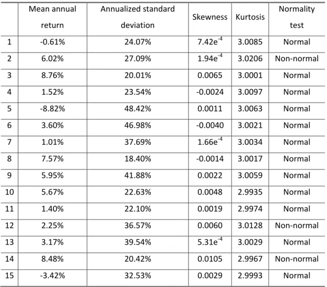
results in samples of normally distributed returns on all 15 securities. On Table II we

Table II – Control Scenario descriptive statistics

Mean annual

return

Annualized standard

deviation

Skewness Kurtosis Normality test

1 -0.61% 24.07% 7.42e-4 3.0085 Normal

2 6.02% 27.09% 1.94e-4 3.0206 Non-normal

3 8.76% 20.01% 0.0065 3.0001 Normal

4 1.52% 23.54% -0.0024 3.0097 Normal

5 -8.82% 48.42% 0.0011 3.0063 Normal

6 3.60% 46.98% -0.0040 3.0021 Normal

7 1.01% 37.69% 1.66e-4 3.0034 Normal

8 7.57% 18.40% -0.0014 3.0017 Normal

9 5.95% 41.88% 0.0022 3.0059 Normal

10 5.67% 22.63% 0.0048 2.9935 Normal

11 1.40% 22.10% 0.0019 2.9974 Normal

12 2.25% 36.57% 0.0060 3.0128 Non-normal

13 3.17% 39.54% 5.31e-4 3.0029 Normal

14 8.48% 20.42% 0.0105 2.9967 Non-normal

15 -3.42% 32.53% 0.0029 2.9993 Normal

As we can observe the majority of the stocks follow a normal distribution. Even the

ones which fail the normality test have skewness very close to 0 and kurtosis close to 3

which demonstrates that they behave in many ways like a normally distributed sample.

Consequently, this first simulation does not contain many outlier observations.

Therefore the main cause of estimation error are the sample size and the high

standard deviation of stock returns, which by themselves can be enough to cause

portfolio allocation inefficiencies. This control scenario allows, in particular, to see if

without extreme observations to bias the inputs of MVT, robust estimators are less

efficient than classical estimators, and if so, how significantly. It is also important to

realized risk/return of all securities on the following year, the true parameters  and

.

3.2.2 Contamination scenario

On the contamination scenario, various sets of 200 resamples are produced. However,

in this case the Monte Carlo simulation does not follow a geometric Brownian motion.

It includes a multiplicative contamination, which consists in randomly multiplying a

certain percentage of the standard normally distributed matrix that is on the base of

the geometric Brownian motion by a certain value, as proposed by Perret-Gentil and

Victoria-Feser (2005). Through this method, it is possible to test the stability of the

Mean Variance portfolios against outlier observations and small parameter

fluctuations. It artificially creates extreme observations typical of financial returns and

adding “noise” to the sample in order for the estimated parameters to fluctuate. This way, we are able to test if a small degree of deviation on the estimated parameters

seriously affects the composition and performance of the tangent portfolios, as well as

testing how both types of estimators behave on the presence of extreme observations.

Nine different contamination scenarios are used on this study, varying in percentage of

sample contamination and in magnitude of contamination. The percentages of

contamination are 2.5%, 5% and 10% and the magnitude of contamination, that is, the

value by which each contaminated return is multiplied, is 2.5, 5 and 10. Each

percentage of contamination is tested with each magnitude, allowing for nine different

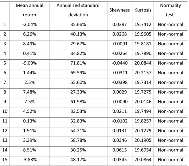
contamination degrees. On Table III we present the descriptive statistics for the

Table III – Contamination Scenario descriptive statistics

Mean annual

return

Annualized standard

deviation

Skewness Kurtosis Normality test3

1 -2.04% 35.66% 0.0387 19.7412 Non-normal

2 6.26% 40.13% 0.0268 19.9605 Non-normal

3 8.49% 29.67% -0.0091 19.8181 Non-normal

4 0.41% 34.82% -0.0264 19.7890 Non-normal

5 -9.09% 71.81% -0.0440 20.0844 Non-normal

6 1.44% 69.59% -0.0311 20.2157 Non-normal

7 2.5% 55.60% -0.0398 19.7314 Non-normal

8 7.48% 27.33% 0.0029 19.7275 Non-normal

9 7.5% 61.98% -0.0090 20.0146 Non-normal

10 4.52% 33.53% 0.0211 19.7494 Non-normal

11 0.13% 32.83% -0.0102 19.8257 Non-normal

12 1.91% 54.21% 0.0131 20.1279 Non-normal

13 3.39% 58.78% 0.0346 20.1905 Non-normal

14 8.51% 30.25% 0.0615 19.6054 Non-normal

15 -3.88% 48.17% 0.0345 20.0864 Non-normal

On opposition with the control scenario, this scenario is composed by 15 non-normally

distributed securities. All stocks present fat tails, as we can see by the high kurtosis.

That means that in this scenario there are many more outlier observations which may

have a great impact on the estimated parameters.

3.3 Robust estimator

On all scenarios, after creating the 200 resamples, there is a need to estimate the

inputs of MVT





multivariate M-estimator which looks into the

2

n h_ _

  observations (out of ) whose

classical covariance matrix has the lowest possible determinant, see Rousseeuw

(1984). The location estimate is then computed by taking the average of those h

points and the scatter estimate is the covariance matrix of those h points. These

estimates can resist





n

  . In extreme cases, in order to achieve the highest

resistance against outliers an  of 0.5 could be used. However, in less extreme

scenarios,  should be set higher than 0.5 in order to improve finite-sample efficiency.

In our case,  was set to 0.75 on all estimations. That means that the estimations

produce stable results if the sample contains up to 25% outliers. Moreover, we have

finite samples and so, in order to achieve a good enough efficiency, an  higher than

0.5 would be needed.

3.4 Portfolio creation process

On this study we work with three different types of portfolios: Tangent portfolios,

average portfolios and, in a lesser extent, naive portfolios. All those portfolios are used

to compare the performance of both estimation styles.

First and foremost, it is important to mention that on each scenario, we have two sets

of portfolios, a set of classically and another of robustly estimated portfolios. After

computing ˆ_i and ˆ_i for n1, , 200 for each estimation type, MVT results in two groups of 200 efficient frontiers. An efficient frontier is a set of efficient portfolios

resulting from MVT. However, we need to find the tangent portfolio for each efficient

frontier. That portfolio is the most efficient portfolio of a given efficient frontier on the

presence of a risk free rate. Having a defined efficient frontier and risk free rate are the

necessary tools to reach the tangent portfolio. The risk-free rate used on this study is

the 12-month Euribor rate at the date of 25/2/15, 0.24%. Euribor is the rate that is

assumed risk-free, following the assumption that the European Central Bank has no

risk of default. The maturity of 12-months is also the one that makes more sense since

as we know the parameters  and  for the next year and the investment horizon of this simulation is one year. Other assumption of this study was the non-inclusion of

short selling on the portfolio creation process. This is consistent with many other

studies on MVT, with the majority of portfolios on the market and it makes the study

simpler and easier to understand. See for example, Chopra and Ziemba (1993) and

Goldfarb and Iyengar (2003).

The second portfolio type is the “average portfolio”. That portfolio is born from the

average weights of all resamples, following the process developed by Michaud (98),

like mentioned on section 2.3. This portfolio will then be compared with the so called

naive portfolio, the portfolio which allocates equal weights for all possible assets.

All those portfolios may differ greatly in risk and return. That is why we need a

performance measure to compare any of them with one another. The instrument used

is the Sharpe Ratio. Developed by William Sharpe, it is a measure of excess return per

unit of risk. It is commonly used in finance and in this study is the major instrument for

4. Results

This chapter starts by presenting a broad view in to the control scenario on section 4.1. Subsequently, it presents the results for the different types of portfolios tested on that scenario, on subsection 4.1.1 we study the behavior of tangent portfolios and on subsection 4.1.2 average and naive portfolios. On section 4.2 the focus is on the contaminated scenario, with a major focus on the 5% contamination. Again, on subsection 4.2.1 we take a look at how tangent portfolios perform on contaminated samples and on subsection 4.2.2 we test how average and naive portfolios perform.

4.1 Control scenario

We build 200 classically estimated efficient frontiers and 200 robustly estimated

efficient frontiers. The resulting efficient frontiers can be observed below, with the

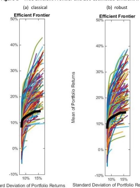
Figure 1 – True Efficient Frontier and 200 estimated efficient frontiers

Figure 1 shows the great variety of estimated efficient frontiers that MVT created,

both by classical and robust estimation. As we could observe on Table II of chapter 3,

the resample process created a huge dispersion of returns on all securities. This, of

course, led to a great dispersion of efficient frontiers. We can also notice that a great

part of the frontiers are above the true efficient frontier, which may be an evidence of the “estimation error maximizer” effect. By overweighing securities with overestimated returns, there is a much greater chance to create efficient frontiers

Visual representation of estimated efficient frontiers and True efficient frontier, represented by the thicker black curve. On (a) 200 classically estimated efficient frontiers and on (b) 200 robustly estimated efficient frontiers

Figure 2 – Tangent Portfolios

4.1.1 Tangent Portfolios

The next step is to look at the composition of the classically estimated and robustly

estimated tangent portfolios on each different sample. On Figure 2 we can see the

distribution of the estimated tangent portfolios’ risk and return, the red line represents the median, the point with the exact number of higher and lower

observations, the edges of the box represent the

25% and 75% percentiles and the upper and lower black lines represent the highest

and lowest observations, respectively. The red crosses represent observations

considered outliers. Additionally, the true tangent risk and return are represented by blue circles. As we can see, classical and robust portfolios present roughly the same

dispersion of observations, both on risk and return. Moreover, approximately 75% of

estimated tangent returns are above the true tangent return of 10.71% and range from around 2% to almost 25%. The estimated tangent risk level is higher than the true risk

level of 14.2% on around 90% of the observations, though it has a much smaller range

of observations, going from 13% to 22%. The great dispersion of tangent returns is

Dispersion of estimated tangent portfolios’ return and risk, both for classical estimation and robust estimation. True optimal return and risk represented by the blue circles.

associated with the already discussed sampling variability associated with the high

standard deviations of the 15 securities. The fact that estimated tangent returns

happen to be much higher than the true tangent return is a reflection of the

“estimation error maximizer” effect of MVT which causes MVT to allocate a greater part of the budget on assets with returns positively affected by estimation error and

less on assets negatively affected with estimation error. Therefore, these assets with

higher estimation error have a higher weight on the estimated portfolio than on the

true tangent portfolio. This results in estimated tangent portfolios with higher return and slightly higher risk than the true tangent portfolio’s risk and return. Concluding, as estimation error on returns has a higher effect on tangent portfolio composition, those

securities with overestimated returns will have more weight on the tangent portfolio

and consequently its tangent return will be overestimated and to a lesser extent its risk

will also be overestimated.

Up to this point, we have been looking at the behavior of the tangent portfolios on

their own simulated samples. Now we study their performance in “reality”. On this

empirical study “reality” is represented by the parameters   _{as in equations (1)}

and (2). By collecting the weights of the estimated tangent portfolios and applying

Figure 3 – Classical risk/return scatter

Figure 4 - Robust risk/return scatter

Figures 3 and 4 show the true position of all tangent portfolios with respect to the

efficient frontier, using both classical and robust estimation. On both cases the true tangent portfolio is represented by an orange circle on the efficient frontier. Looking at

Scatter of the risk/return of 200 classically estimated tangent portfolios, on the true efficient frontier plus the true tangent

portfolio, represented by an orange circle.

Scatter of the risk/return of 200 robustly estimated tangent portfolios, on the true efficient frontier plus the true tangent portfolio,

the scatter we can notice that all estimated tangent portfolios result in less than

optimal portfolios on practice. This happens due to the fact that the estimated

parameters (ˆi ˆi j j

  ),i(classical robust, ), j(1, , 200)) which served has base for its computation had an associated estimation error. Combining this with the

“estimation error maximizer” effect of MVT referred to on section 2.2, lead to tangent portfolios which overweighted securities with overestimated returns and

underestimated standard deviations, and vice versa. As estimation error is positively

correlated with standard deviation and in this study all 15 securities present high

standard deviations is easy to understand the cause of the large range of risk/returns

and consequent inefficiency presented by these estimated portfolios.

Even if Figure 3 and 4 give us an idea about how estimated tangent portfolios behave

on the following year, visual inspection is not enough to reach solid conclusions.

Therefore, there is a need to measure the performance of each portfolio through the

Sharpe ratio. The true tangent portfolio has a Sharpe Ratio of 0.7373. That portfolio is the point of the efficient frontier that maximizes the Sharpe Ratio for the defined risk

free rate. All the estimated portfolios are under that same efficient frontier. Thus, it

can be instantly affirmed that all estimated portfolios have a lower Sharpe Ratio than

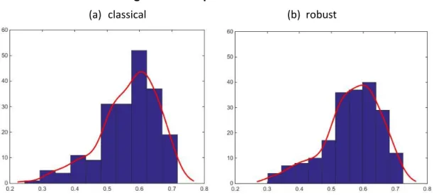
the true tangent portfolio. This statement was then confirmed by computing each portfolio Sharpe Ratio, see Figure 5. In order to compare both estimation methods

with each other and with the true tangent portfolio an average of each of the 200 portfolios Sharpe Ratio was taken.

Figure 5 – Sharpe Ratio distribution

The results show that on average a classically estimated tangent portfolio has a

Sharpe of 0.5654 and a robustly estimated tangent portfolio has a Sharpe of 0.5643.

The classical estimation leads to a marginally higher performance measure. This

confirms the theory of robust statistics, which defines robust estimators as less

efficient estimators on a well distributed sample, that is, a sample without outlying

observations as is the case on this first scenario, see Table II. Additionally, classically

estimated portfolios have a standard deviation of its Sharpe ratio of 0.0852 against

0.0929 of robustly estimated portfolios. This adds to the point that robustly estimated

portfolios are less efficient than classically estimated ones. What can be concluded

from these results is that when building a portfolio through MVT, on a sample without

any outlying observations, classical estimation is marginally more efficient than robust

estimation.

4.1.2 Average and naive portfolio

On this study we have the opportunity of creating portfolios through the resampling

method developed in Michaud (1998). Doing an average of the weight each security

has on the 200 tangent portfolios, both for the classical and robust case, results in two

average weighted portfolios, one for the classical estimation and another for the

robust estimation, see Figure 6.

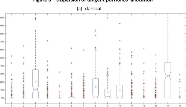
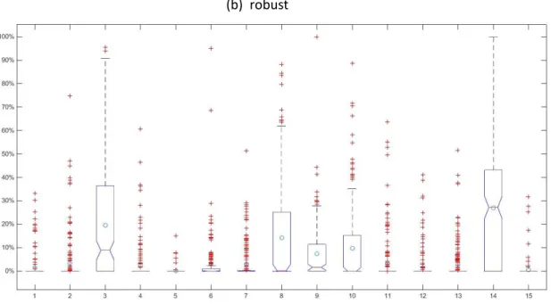
Figure 6 –Dispersion of tangent portfolios’ allocation

If we apply those two portfolios to the true efficient frontier we can see how those average weighted portfolios behave on practice and compare it with the behavior of a

naively created portfolio. That behavior can be observed below on Figure 7:

Figure 7 – Average and Naive Portfolios

Average weighted, naive and true tangent portfolios on the true efficient frontier. The green circle represents the true tangent portfolio. The red cross represents the average robust portfolio. The orange Dispersion of the tangent portfolio weights of each asset on the 200 resamples, both for classical estimation (a) and robust

The orange diamond represents the average weighted classical portfolio and the red

cross inside it represents the average weighted robust portfolio. Additionally, the

green circle on top of the true efficient frontier is the true tangent portfolio and the blue dot on the bottom is the naive portfolio, with an equally weighted allocation

between the 15 securities. As we can see, both classical and robust portfolios are

below the efficient frontier, though having a higher return and lower risk than the

naive portfolio. Also, they present roughly the same risk and return, which shows that

robust estimators are as good as classical estimators in an environment where they

were expected to be less efficient. Looking at each portfolio’s Sharpe ratio, we can confirm that both estimators result in equally efficient portfolios as they have exactly

the same Sharpe ratio of 0.6848, not too far from the Sharpe ratio of the true tangent portfolio of 0.7373. Another fact worth considering is that a Sharpe ratio of 0.6848 is way higher than the average Sharpe calculated beforehand for the 200 classically

estimated portfolios (0.5403) and 200 robustly estimated portfolios (0.5354). This

happens because by doing the average of the weights of the 200 portfolios, we are

mitigating the error maximization effect caused by estimation error. If in some

portfolios certain assets’ weights were overestimated, on other portfolios the same

assets’ weights might have been underestimated, assuming that there is the same chance of happening positive and negative estimation errors. So, by doing the average

of those weights we are nullifying the overestimations with the underestimations and

reaching closer to the true tangent portfolio performance.

4.2 Contamination Scenario

On a second stage, the resampling process was repeated for the contamination

scenario. Again, two methods of evaluating the performance of both estimators are

developed. Firstly we put each of the 400 estimated tangent portfolios (200 classical

portfolios, apply those portfolios on the true efficient frontier and then look at its Sharpe ratio. In this part the focus is on the contaminations of 5% of observations by

the three magnitudes of contamination of 2.5, 5 and 10. On annex the same results for

the 2.5% and 10% contaminations can be observed.

4.2.1 Tangent portfolios

Let’s start by looking at the distribution of risk/return of both classical and robust estimated tangent portfolios for the three magnitudes of contamination on Figures 8,

9 and 10:

Figure 8 - Dispersion of estimated tangent portfolios (5% contamination 2.5 magnitude)

Figure 9 - Dispersion of estimated tangent portfolios (5% contamination 5 magnitude)

Dispersion of tangent portfolios’ return (a) and risk (b) on the 5% contamination, 2.5 magnitude scenario. The blue circles represent the true tangent portfolio return and risk, respectively

(a) return (b) risk

Figure 10 - Dispersion of estimated tangent portfolios (5% contamination 10

magnitude)

The red line represents the median, which is the observation that has the same

number of higher and lower observations, the top and bottom blue lines represent the

75% and 25% percentiles, respectively. The black line on top represents the higher

observation and the bottom black line the lower observation. Additionally the red

crosses are observations treated as outliers and the blue circle represents the

expected return and risk of the true tangent portfolio. Identically to the base scenario the estimated expected returns of the three contaminations are around 75% to 80% of

the times higher than the true expected return and the risk almost always higher than the true risk. On the 2.5 magnitude contamination there are no noticeable differences between the classical and the robust estimator, which tells us that a magnitude of 2.5

is not enough to produce extreme enough observations on these samples. However, as

the magnitude of contamination increases we can identify a pattern of growth and

dispersion of the classically estimated portfolios, both on expected return and risk. In

opposition robustly estimated portfolios maintain roughly the same distribution of

risk/return on all magnitudes. This is a proof of the ability of robust estimators to

produce stable results even in situations where the sample is not a good source of

information for the parameters needed due to the presence of outlying observations

or in situations when some securities parameters fluctuate.

(a) return (b) risk

Dispersion of tangent portfolios’ return (a) and risk (b) on the 5% contamination, 10 magnitude scenario.

Now it is important to apply the weights of each portfolio to the true efficient frontier

in order to observe how they will perform on the next year. On the following table we

can see the average of the Sharpe ratios of the classically and robustly estimated

portfolios with 2.5%, 5% and 10% contamination under the three different

magnitudes.

Table IV – Sharpe Ratio of tangent portfolios on the true efficient frontier

Sharpe Ratio

–

2.5% contamination

Magnitude

Classical Robust

Mean Standard

deviation

Mean Standard

deviation

2.5 0.5566 0.0963 0.5499 0.1058

5 0.5342 0.0919 0.5494 0.0851

10 0.5055 0.1055 0.5338 0.0966

Sharpe Ratio

–

5% contamination

Magnitude

Classical Robust

Mean

Standard

deviation Mean

Standard

deviation

2.5 0.5587 0.0881 0.5525 0.0864

5 0.5217 0.1152 0.5370 0.1047

10 0.4823 0.1061 0.5262 0.1078

Sharpe Ratio

–

10% contamination

Magnitude

Classical Robust

Mean Standard

deviation

Mean Standard

deviation

2.5 0.5395 0.0965 0.5337 0.1025

5 0.4958 0.1025 0.5034 0.1042

10 0.4520 0.1058 0.4823 0.1068

To start, is important to note that again all the estimated portfolios are below the true efficient frontier and so, none of them presents a Sharpe ratio equal or higher than the ratio of the true tangent portfolio (0.7373). Looking at Table IV, we can see that for the lower magnitude classically estimated portfolios present a higher Sharpe ratio than

robustly estimated portfolios. That difference is marginal and confirms that this lower

magnitude is not enough to create extreme enough observations in order for robust

estimators to perform better than classical estimators. However, as the magnitude

increases we can see that the average Sharpe ratio of classically estimated portfolios

decreases much more than the Sharpe of robustly estimated portfolios which proves

that on the 5 and 10 magnitudes of contamination robust estimation is a much more

viable tool to create mean variance portfolios on an environment without a well

distributed sample. On the 2.5% contamination the pattern of decline of Sharpe ratio

as the magnitude increases is common with the 5% contamination. Again, on the 2.5

magnitude classically estimated portfolios present a slightly higher Sharpe ratio but on

the two higher magnitudes robustly estimated portfolios have a higher Sharpe ratio,

which remains stable as the magnitude increases. On the 10% contamination we can

observe that once more on the 2.5 magnitude classically estimated portfolios have a

marginally higher Sharpe ratio but on the other two magnitudes robustly estimated

portfolios have a higher Sharpe. However, on this higher percentage of contamination

we can see that the robustly estimated portfolios’ average Sharpe ratio is not stable. As the magnitude of contamination increases, the average Sharpe ratio decreases

considerably, perhaps due to the inability of the robust estimator to deal with the total

amount of outlying observations present on that extreme scenario of contamination.

4.2.2 Average and naive portfolio

Repeating the same process of averaging the weights of the various estimated

portfolios on the 5% contaminated samples and for all three magnitudes, we produce

one average weighted classical portfolio and one average weighted robust portfolio for

each magnitude. Once more, on Figure 11 we have the true efficient frontier, the true tangent portfolio represented by a green circle, the average weighted classical portfolio represented by an orange diamond, the average weighted robust portfolio

Figure 11 - Average and Naive Portfolios

(a)

(b)

(c)

On the 2.5 magnitude the two average weighted portfolios seem to have roughtly the

same risk/return, though the classically estimated portfolio has a Sharpe ratio of 0.673

compared with a Sharpe ratio of 0.6693 of the robustly estimated portfolio. This fact is

consistent with the previous considerations taken, namely that a magnitude of 2.5 is

not enough to create significant outlying observations which would create “noise” on the sample. On the opposite side, the 5 and 10 magnitudes displays a decrease in

performance by the average weighted classical portfolio. As the magnitude increases

the classical portfolio’s Sharpe ratio decreases considerably, as can be observed on Table V:

Table V – Sharpe Ratio of average portfolios

Sharpe Ratio

Magnitude

2.5% contamination 5% contamination 10% contamination

Classical Robust Classical Robust Classical Robust

2.5 0.679 0.6726 0.673 0.6693 0.6585 0.6533

5 0.6499 0.6743 0.6329 0.6475 0.5995 0.6061

10 0.6017 0.6483 0.5713 0.6553 0.5382 0.5728

Once again, averaging the weights of the different estimated portfolios provides

portfolios with a much higher performance than the average Sharpe of each estimated

portfolio. Additionally the average weighted robust portfolio remains stable with an

increase in magnitude, as opposed to the average weighted classical portfolio. Another

proof of the stability of robust methods of estimation to outlying observations and

distancing of the sample from the realized risk/return. On the 2.5% and 10%

contaminations the pattern remains. On the 2.5% contamination, average weighted

classical portfolios decrease as the magnitude increases, when average weighted

robust portfolios remain stable. On 10% contamination both classes of portfolios

decrease as the magnitude increases, though the decline on average weighted classical

portfolios Sharpe ratio is higher than the decline on average weighted robust

portfolios.

5. Conclusion

Mean Variance Theory is based on the assumption that expected returns and

covariances between securities are the only necessary inputs in to create efficient

portfolios. These inputs are not known, have to be estimated and are therefore subject

to estimation error. This puts a great importance on the estimation process. This study tests the ability that two possible estimators (classical maximum likelihood estimators

and robust estimators) have to withstand outlying observations which may have a

higher than desired effect on the parameter estimation, and to withstand small

parameter deviations and still remain stable. With the meaning of stable being: to

produce close to efficient portfolios on majority of the possible scenarios. It can be

stated that on scenarios of uncertainty, where the sample may not be a perfect source

of information for the estimation of the parameters needed for MVT, robust

estimators produce closer to optimal results than classical estimators. Only on the

scenarios where the sample is a close to perfect reflection of the true parameters do classical estimators produce better results than robust estimators. However, the

results that classical estimators produce on these situations are only marginally

superior, whereas on the extreme contamination scenarios, where the sample doesn’t exactly represent the true parameters and contains many outlying observations, robust estimators have a much higher performance. Which makes robust estimation a

good tool of risk mitigation, as it produces close to efficient results even on the worst

case scenario. In comparison, classical estimation produces slightly more efficient

results but only on the best case scenario. Future research might study the

performance of different types of robust estimators against on another, try to study

which contamination percentage and magnitude would be a better reflection of the

uncertainty observable on financial data. Other possible developments would be to

repeat the simulation process with another distribution or apply a different weight to

References

Barry, C. B. (1974). Portfolio analysis under uncertain means, variances, and covariances. The

Journal of Finance, 29(2), 515-522.

Bawa, V. S., Brown, S. J., & Klein, R. W. (1979). Estimation risk and optimal portfolio

choice. NORTH-HOLLAND PUBL. CO., N. Y., 190 pp.

Ben-Tal, A., & Nemirovski, A. (1998). Robust convex optimization.Mathematics of Operations

Research, 23(4), 769-805.

Best, M. J., & Grauer, R. R. (1991). On the sensitivity of mean-variance-efficient portfolios to

changes in asset means: some analytical and computational results. Review of Financial

Studies, 4(2), 315-342.

Black, F., & Litterman, R. B. (1991). Asset allocation: combining investor views with market

equilibrium. The Journal of Fixed Income, 1(2), 7-18.

Brown, S. J. (1976). Optimal portfolio choice under uncertainty: A Bayesian approach (Doctoral

dissertation, University of Chicago, Graduate School of Business).

Chopra, V. K. (1993). Improving optimization. The Journal of Investing, 2(3), 51-59.

Chopra, V. K., & Ziemba, W. T. (1993). The effect of errors in means, variances, and

covariances on optimal portfolio choice.

El Ghaoui, L., & Lebret, H. (1997). Robust solutions to least-squares problems with uncertain

data. SIAM Journal on Matrix Analysis and Applications, 18(4), 1035-1064.

Goldfarb, D., & Iyengar, G. (2003). Robust portfolio selection problems.Mathematics of

Operations Research, 28(1), 1-38.

Hampel, F. R. (1968). Contributions to the theory of robust estimation. University of California.

Hampel, F. R. (1974). The influence curve and its role in robust estimation.Journal of the

American Statistical Association, 69(346), 383-393.

Hampel, F. R. (1986). Ronchetti, EM, Rousseeuw, PJ, and Stahel.

Huber, P. J. (1964). Robust estimation of a location parameter. The Annals of Mathematical

Statistics, 35(1), 73-101.

Huber, P. J., & Ronchetti, E. M. (1981). Robust StatisticsWiley. New York.

Jobson, J. D., Korkie, B., & Ratti, V. (1979). Improved estimation for Markowitz portfolios using

and Economics Statistics Section(Vol. 41, pp. 279-284). American Statistical Association

Washington DC.

Jobson, J. D., & Korkie, R. M. (1981). Putting Markowitz theory to work. The Journal of Portfolio

Management, 7(4), 70-74.

Jorion, P. (1986). Bayes-Stein estimation for portfolio analysis. Journal of Financial and

Quantitative Analysis, 21(03), 279-292.

Kolm, P. N., Tütüncü, R., & Fabozzi, F. J. (2014). 60 Years of portfolio optimization: Practical

challenges and current trends. European Journal of Operational Research, 234(2), 356-371.

Lobo, M. S., & Boyd, S. (2000). The worst-case risk of a portfolio. Unpublished manuscript.

Available from http://faculty. fuqua. duke. edu/% 7Emlobo/bio/researchfiles/rsk-bnd. pdf.

Lintner, J. (1965). The valuation of risk assets and the selection of risky investments in stock

portfolios and capital budgets. The review of economics and statistics, 13-37.

Markowitz, H. (1952). Portfolio selection*. The journal of finance, 7(1), 77-91.

Markowitz, H. (1959). Portfolio selection: efficient diversification of investments. Cowies Foundation Monograph, (16).

Merton, R. C. (1980). On estimating the expected return on the market: An exploratory

investigation. Journal of Financial Economics, 8(4), 323-361.

Metropolis, N., & Ulam, S. (1949). The monte carlo method. Journal of the American statistical

association, 44(247), 335-341.

Michaud, R. O. (1989). The Markowitz optimization enigma: is' optimized'optimal?. Financial

Analysts Journal, 45(1), 31-42.

Michaud, R. O., & Michaud, R. (1998). Efficient asset management. Harvard Business School

Press, Boston.

Mossin, J. (1966). Equilibrium in a capital asset market. Econometrica: Journal of the

econometric society, 768-783.

Perret-Gentil, C., & Victoria-Feser, M. P. (2005). Robust mean-variance portfolio

selection. Available at SSRN 721509.

Reilly, F. K. (1985). Investments Analysis and Portfolio Management. Dryden Press, San

Francisco.

Rousseeuw, P. J. (1984). Least median of squares regression. Journal of the American

Sharpe, W. F. (1966). Mutual fund performance. Journal of business, 119-138.

Stein, C. (1956). Inadmissibility of the usual estimator for the mean of a multivariate normal

distribution. In Proceedings of the Third Berkeley symposium on mathematical statistics and

probability (Vol. 1, No. 399, pp. 197-206).

Ter Horst, J., De Roon, F., & Werker, B. J. (2002). Incorporating estimation risk in portfolio