INANCE 20152016 MASTER ’ S FINAL WORK

MASTERS

FINANCE 2015/2016

MASTER

’

S FINAL WORK

D

ISSERTATION

T

HE

V

ALUE OF

I

NFORMATION

:

T

HE

I

MPACT OF

EBA

S

TRESS

T

ESTS

IN

S

TOCK

M

ARKETS

A

NDRÉ

A

LEXANDRE

G

ALHETO

P

EREIRA

S

:

P

.

D

.

J

M

Z

M

C

-S

:

D

.

G

A

BANCO DE PORTUGAL,DEPUTY DIRECTOR, RISK MANAGEMENT DEPARTAMENT

2

THE VALUE OF INFORMATION: THE IMPACT OF EBA

STRESS TESTS IN STOCK MARKETS

3

Acknowledgement

I would like to express my gratefulness to my supervisor, Prof. José Manuel

Zorro Mendes, for his help in the process of this dissertation.

I also thank to Dr. Gabriel Andrade from Banco de Portugal for his remarkable

and insightful comments. Additionally, to Prof.ª Isabel Proença for her assistance.

I also thank my girlfriend for her support and encouragement along the way.

In a special note, I dedicate this work to my parents and grandparents, to

4

"Stress testing is a key tool to ensure that financial companies have enough

capital to weather a severe economic downturn without posing a risk to their

communities, other financial institutions, or the general economy."

5

List of abbreviations

Abbreviation

Name

CDS

Credit Default Swap

CEBS

Committee of European Banking Supervisors

EBA

European Banking Authority

EC

European Commission

ESRB

European Systemic Risk Board

6

Index

1. Introduction ... 9

2. Literature Review... 13

3. Data and Methodology ... 17

4. Results ... 21

4.1 Announcement Event ... 21

4.2 Methodology Event ... 22

4.3 Results Event ... 23

4.4 The 2014 Stress Test ... 23

4.4.1 Banks above the minimum requirement ... 24

4.4.2 Banks below the minimum requirement ... 24

4.5 Additional Insights ... 25

5. Conclusion... 27

References ... 29

7

Table Index

Table I –Events’ dates ... 19

Table II – Sample of Banks ... 32

Table III – Descriptive Statistics for all Samples ... 32

Table IV – Announcement Event for entire sample ... 33

Table V – Methodology Event for entire sample ... 34

Table VI – Results Event for entire sample ... 35

Table VII – All Events for sample above the threshold in 2014 ... 36

Table VIII - All Events for sample below the threshold in 2014 ... 37

Table IX – Announcement Event for entire sample without temporary effect ... 38

Table X – Methodology Event for entire sample without temporary effect ... 38

Table XI – Results Event for entire sample without temporary effect ... 39

Table XII – All Events for sample above the threshold in 2014 without temporary effect ... 39

8

Abstract

This dissertation focus in testing if the 2010, 2011 and 2014 European Stress

Tests performed under CEBS and EBA supervision produced useful and real

information to the market.

Using an augmented CAPM model, I found that the most significant event to

the stock markets is the Methodology release, in terms of risk and returns. In

contrast, the Results event did not have much impact in the same market when

considering the entire sample as one. Yet treating the sample in two different

groups, on one hand the banks that passed and on the other hand the banks that

failed, we can observe a significant reaction of the stock markets in the last group.

These findings are consistent with the literature available which conclude that

the stress tests provide real and valuable to the markets about the banking

9

1. Introduction

The year of 2008 was the key moment for banking regulation.

The financial crisis increased the exposure and scrutiny to the banking system

due to the collapse of the well-known American banks such as Lehman Brothers

and Bear Stearns but also due to the sovereign debt crisis in Europe. Was this

financial crisis triggered by a lack of regulation?

In response, central banks improved an already existing tool: the stress tests.

These tests are based on a simulation methodology like, for example, Monte

Carlo’s simulations, a technique to predict the future and use that scenario to

forecast results. The stress tests are also made under unfavourable economic

scenarios in order to determine if a bank has (or not) sufficient capital to

accommodate the impact on their balance sheet.

The main objectives of a stress test are preventing the undercapitalization of

the banking sector, valuating the bank’s loss absorbing capacity, identifying

vulnerabilities in bank’s risk management strategy, providing valuable

information to regulators and at the same time increase the confidence,

predictability and security in the financial markets.

The construction of the scenarios does not take into account historical data

and does not expect past observations to remain valid in the future. The correct

approach is forecasting possible developments in the economy and try to predict

10

One of the main targets of the European regulators was to restore the

confidence on Europe’s economy and banking sector, signalizing to the market

that they are aware of the problems that can happen in the future of the banking

industry.

The European institutions introduced widespread stress tests in 2010 led by

the Committee of European Banking Supervisors (CEBS) and since 2011

performed by the European Banking Authority (EBA) replacing CEBS.

The 2010 exercise was conducted in 91 European banks, covering at least 50%

of the evaluated countries banking sector and also representing 65% of the

European banking industry total assets.

The minimum threshold adopted to pass in the test was 6% of Core Tier 1 ratio

for the adverse scenario. A value that 7 banks failed to achieve. The general

perception was that this test was relatively poorly received giving the wrong

insight to the market. The reason for this scepticism was the release of limited

information contributing to increase the already existent uncertainty at that time

in the markets. It was unanimous from the financial institutions to the general

society that the adverse scenario adopted was not reasonable or even considered

“adverse” since it only assumed a 0.6% decrease in GDP (Gross Domestic

Product). This led to a subjective result where banks not well capitalized and not

11

these banks a few months after were asking for public intervention to support

their business.

The 2011 stress test, the first performed by EBA, was seen as a successful

reinforcement and upgrade to the 2010 test, namely by increasing the severity of

the adverse scenario – assuming now a drop of 4% in GDP – as well as the

disclosure and transparency of the methodology and data used which

contributed to an improvement of the results reliability. The sample was

composed by 91 banks (however, only 90 were disclosed) and the threshold was

changed to 5% of Core Tier 1 ratio which caused 20 banks to fall below this level

and consequently fail the test.

A lesson to bear in mind with these tests is when the data and methodology

used is public the market can conduct their own tests and methodologies

contributing to eliminate the doubt among the investors.

In 2014, EBA added an additional tool - the Asset Quality Review (AQR) - to

complement the stress tests and improve the information provided to the market

therefore reducing the systemic risk. The baseline and adverse scenarios were

developed by European Systemic Risk Board (ESRB) and the European

Commission (EC). The sample had increased to 123 banks and the threshold for

the adverse scenario was set at 5.5% of Core Tier 1 ratio. In total, 24 banks had

failed to reach the minimum required. The latest tests were considered by the

12

Although they were the best tests they were still referred as "a walk in the park

on a Sunday morning" by Saxo Bank's Chief Economist when comparing with the

American stress tests which are far more developed.

However, are these tests really helping the regulators? Are they real enough

to warn the system about damaging banks? Are they contributing to reduce the

risk in the market or on the other hand is it helping to increase the distrust in the

system? If the probability of the worst scenario is extremely low would be this

best scenario to test and would it increase the confidence on the markets?

This dissertation aims to test the impact of the 2010, 2011 and 2014 Europe’s

Stress Tests events – Announcement, Methodology and Results release events -

on the stock markets, measuring their impact to reduce or increase the risk and

also testing for the presence of abnormal returns.

The main objective is to answer the following questions:

I. Is the short term risk of the bank’s stocks impacted by any of these events?

II. Is the long term risk of the bank’s stocks impacted by any of these events?

III. Is there any abnormal stock’s return evidence on any of these events?

We will also compare the results to the same questions on the 2014 stress test

but dividing the sample in 2 groups – the banks that passed and the ones that did

13

With this work we aim to contribute to the discussion about the effectiveness

and real impact of these tests on the European banking system. Are they

contributing to increase the efficiency of the market? Are they helping to improve

the information for the investor?

This dissertation is organized as follows. Section 2 presents a review of the

literature that studied this topic regarding the Stress Test in last years but with

other different approaches, methodologies and geographically diversified. Those

works also cover different geographies. Section 3 shows how the data for this

work was defined and which methodology was followed. In this section we also

describe the methodology used. The Section 4 contains the results of this work

showing how the banking system was impacted by the stress tests analysed and

also gives additional and important insights with analysis in different viewpoints.

Section 5 gives concluding remarks, further points to work and limitations of this

14

2. Literature Review

The literature in this area is increasing due to the recent developments in this

topic by regulators and the banks. The literature mainly focuses on the American

and European stress tests but there is some works with local supervisors. This

thesis tries to contribute a little more to improve the currently information

available on this subject.

The market in general but specially “…the banking system needs indicators

that can serve as warning systems to identify potential bank failures in an efficient

and accurate matter (Apergis, N. et al 2013)”.

One of the tools chosen to produce those important warnings signals were the

stress tests, identified as an essential component on the design of an optimal

disclosure of information between the banking authorities (the regulators) and

the investors (the market) (Gick & Pausch, 2012).

The main technique used to evaluate the impact of certain events such as

mergers, stock splits, etc. is the event study methodology. Peristian et al. (2010)

and Neretina et al. (2014) studied different topics using this technique.

This methodology divides the sample in two windows – the estimation

window and the event window – and then following a model such as a CAPM the

authors try to observe abnormal returns that are defined as the actual return

15

The 2009 US Stress tests were the first widespread exam performed in the

world and as Peristian et al. (2010) found that test provided crucial information

to the market and reduce the opaqueness in banks. The conclusions reached that

the banks facing larger capital gaps on their results are the ones experiencing

higher negative abnormal returns. As a consequence, contributing to increase the

flowing of capital from the riskier to the safer banks as a result of the stress tests

outcomes.

Neretina et al. (2014) studied the impact of 2009 US Stress Test on systematic

risk, equity returns and CDS spreads on 2009-2013 period, reaching the

conclusions of a statistically weak suggestion of impact on equity returns, but a

significant evidence regarding the decline of CDS spreads after the results

disclosure and the decrease of systematic risk in the following years after the

stress test.

Apergis & Payne (2013) with 2011 EBA Stress test as the relevant event

indicated that both credit risk and macroeconomic factors such as lower GDP

growth, higher CDS spreads or higher LIBOR spreads are significant determinants

of bank failures, which can serve as an alert system to the market regulators and

banks itself.

Ellahie (2013) states that “announcement of forthcoming public disclosure and

the eventual disclosure can induce changes in the information environment”.

16

distinct feels: the information asymmetry declined and the information

uncertainty increased. Overall, the author emphasizes the transparency and

credibility as the most important factors of a successful stress test, contributing

to maximize the value of information and the confidence given to the market by

the regulatory institutions.

Alves et al. (2014) concluded that the 2010 and 2011 stress tests brought new

information to the market environment and the outcomes were not anticipated

by the stock market but were partially anticipated by the CDS market. Both

markets had a stronger reaction in riskier financial institutions than in the safer

ones and a positive and immediate influence on the aggregate behaviour of the

sector. The share prices of the banks that passed the tests experienced higher

positive cumulative abnormal returns, leading to a conclusion that investors

attributed value to the information provided in these tests, which is consistent

with what Gick & Pausch (2012) defended 2 years before: “…stress tests create

value as they will generally improve information disclosure between supervisor

and investors”.

Petrella & Resti (2012) defend that the 2011 EBA Stress Test results event was

considered relevant by investors, impacting the stock prices. The authors also

argue that the market is not able to anticipate the test’s results which is

17

shown again the importance of a stress test in producing valuable information to

the market.

Nijskens & Wagner (2008) studied the impact of a CLO and CDS issuance

events on the banks’ risk. This study found a relationship between these events

and the increase of the banks’ beta share price. The increase on banks’ risk was

due to the increase in correlation across banks and not the volatility of the

individual banks, which decreases instead. Overall, these events found an

increase in risk on the financial system but a decrease on the banks’ individual

risk.

Cardinali & Nordmark (2011) concluded that the banks are opaque to an

intermediate degree, sustaining this idea with the fact that 2010 Results and 2011

Clarification events were uninformative to the stocks market but in contrast the

2011 Methodology release event was very informative. In addition, the authors

performed tests distinguish between the PIIGS and Non-PIIGS countries,

18

3. Data and Methodology

The purpose of this thesis is to analyse the impact of the Stress Tests

performed by European institutions on stock market’s indicators, such as the risk

and stock’s return. By comparing the results across different moments and years

we will confirm or refuse the hypothesis that the information given to the market

is reducing the risk and not creating abnormal returns since the stress tests are

supposedly getting more realistic.

With the purpose of explaining the impact of Stress Tests on the stock markets

the main econometric technique that will be used in this dissertation will be the

regression analysis computed with dummies in order to signalize the events

window as well as the interaction between the market return and the applied

dummies, to measure the risk associated to the events considered.

In order to compute the regressions, we collected 2 samples on the banks’

stocks1– one from 18/06/2009 to 26/10/2015 and another one from 18/12/2009

to 26/04/2015, 6 months and 1 year before and after the first and last event being

studied in this dissertation, respectively. All the share prices were collected from

the Bloomberg platform. In the case of some prices being unavailable we filled it

1_{The initial idea for this dissertation was also to study the impact of these events on the Credit Default Swaps}

markets along with stock markets. The absence of historical prices on an appropriate index to be use as proxy of the

19

with the last available stock price. We dropped all banks for which no (or

incomplete) data was available and we considered only the banks that were

involved the three stress tests to give consistent results since the entities

analysed are the same, avoiding to compare different samples for each stress test

and also doing the analysis for banks that are not currently existing since they

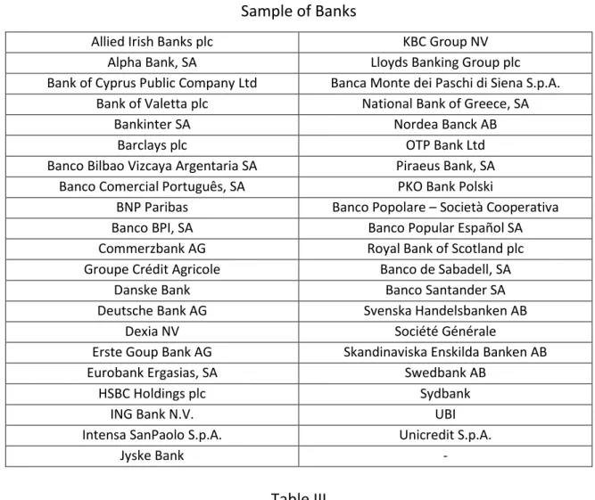
merged or were purchased. This left us with a final sample of 41 banks (Table II).

The descriptive statistics are presented in Table III.

To calculate the stock returns across all data we used the

constant-mean-return model, taking the logarithm as below:

_{𝑅𝑖,𝑡 = ln⁡(} 𝑃𝑖,𝑡

𝑃𝑖,𝑡−1) (1)

Where Ri,t is the log-return for firm i at time t, Pi,t is the current closing price

and Pi,t is last day’s closing price.

The continuous compounded returns were used in order to avoid issues with

nonstationary in the data because it can lead to some severe unreliable test

statistics.

To measure the impact of the events and following Nijskens and Wagner

(2008) we estimated the relationship between the stress tests events and the

bank’s beta in stock markets using the below augmented CAPM model:

20

In the model above, αi is the bank fixed effect and Ri,t and RM,t are the returns

on an individual bank and the market used as a proxy, respectively. The market

return used is measured by the Stoxx Europe Banks 600 Index, an index

containing the majority of the banks in the sample of this study since this index

includes the 600 banks with the largest market capitalization in Europe. Apart

from a significant weight of UBS (a Swiss bank not used in this work) on this index,

all the rest of significant banks (above 3.5% of the index) were part of this

analysis, leading me to choose it as the better one to use as proxy. Dabn _{is a dummy}

variable that takes the value of one 22 business days before and after the event

date and value zero otherwise, measuring any abnormal return associated with

the event. We considered 22 business days in order to have a short time period

to test the impact of the stress test events. However, an interesting work would

also be testing the presence of abnormal returns with less days considered. That

could lead to different results and conclusions. With less days, the impact of the

stress tests should have a bigger importance than the one that will be noticed in

this dissertation. This can lead us to talk about market efficiency: if the markets

are efficient, the adjustment of the security’s price will be almost automatic.

21 Table I

Events’ Dates

Event Date

2010 Announcement 18/06/2010

2010 Methodology 07/07/2010

2010 Results 23/07/2010

2011 Announcement 13/01/2011

2011 Methodology 18/05/2011

2011 Results 15/07/2011

2014 Announcement 31/01/2014

2014 Methodology 29/04/2014

2014 Results 26/10/2014

Dtemp _{is another dummy which takes the value of one in the 66 business days}

before and after the event window. This dummy was used to measure any

temporary beta effect of the event in a short time perspective. On this case we

picked 66 business days to try to capture the temporary effect on risk but with

also with a sufficient range to measure that impact correctly. Dperm _{is the last}

dummy to measure the permanent beta effect, whose value is one from the

event’s date until the end of the period in this work.

The most relevant variables in this regression are the coefficients of the

interaction terms Dtemp_{*RM,t and D}perm_{*RM,t whose measures} the change in a bank’s

22

in comparison to the market, respectively. The beta share price stands for a

measure of a security’s volatility, meaning that a higher beta indicates a higher

volatility, so a higher risk associated with that security. In this model these are

critical variables since we will try to verify an increase or decrease of the risk

associated on the groups of banks analysed. It is expected that the banks who

failed the test experienced an increase on their risk and for the banks who passed

is expected a decrease or neutral effect in their risk.

Denote that these dummies are overlapped (permanent effect and temporary

effect dummies have the same sample in the first 66 business days), meaning that

the permanent effect will take into account the temporary effect. Therefore, we

should exclude the last one from the permanent so that we eliminate the

influence of the temporary on the permanent.

To test the impact of the tests on risk and abnormal return variables we

considered as hypotheses the following:

(Abnormal Return) H0: _{𝛿 = 0} H1: _{𝛿⁡ ≠ 0}

(Temporary Effect on Risk) H0: _𝛽3𝐷𝑡𝑒𝑚𝑝_{= 0 H1: 𝛽}

3𝐷𝑡𝑒𝑚𝑝≠ 0

23

Throughout the dissertation, I will compare all the moments across the three

tests and the impacts on the stock markets as an alternative proxy of the

24

4. Results

The results are present in tables IV, V and VI for the Announcement,

Methodology and Results events, respectively.

In all regressions the market daily return coefficient is statistically significant

at 1% level indicating a high linearity, as expected, between the market used as

proxy – Stoxx Europe Banks 600 Index - and the daily return of the sample used

on this dissertation. The market return coefficient is always above 1

demonstrating that the sample of banks used in this work outperformed the

market. As a curiosity, the constant term is statistically significant at least at 10%

significance in all events on 2014 stress test.

In addition, we verify a probability F-statistic of zero, confirming that the

variables are all jointly significant and the regressions used fits the data well.

4.1 Announcement Event

Regarding the Announcement’s events (Table IV), we verify very small but

statistically significant abnormal returns in 2011 at 10% significance level and in

2014 at 5% level. This confirms the better reaction of the market to the 2014’s

Stress Test comparing to the ones performed in 2011 and 2010.

The temporary effect on beta share price is statistically significant at 10% in

2011 with 6 months’ data, having an impact of approximately -0.0557 on it. Even

25

of signal after the 2010 stress test from an increase to a decrease on its risk, in

the 2011 and 2014 tests.

4.2 Methodology Event

In Methodology events (Table V) we found statistically significant abnormal

returns in all regressions except one, the 6 months’ data in 2010 test. Yet they

have different interpretations between them. The evidence shows that the

Methodology release had a higher influence on the stock markets in comparison

to the Announcement event. The 2010 test outputs a small positive abnormal

return below 0.1% at 10% significance level. The market did not find the tests as

being a real inspection on the banks. In 2011 and 2014 these methodologies

releases were differently assumed by the market, turning to small negative

abnormal returns statistically significant at level of 5%. This negative impact on

the returns of the bank’s stocks occurred because the market’s fear the scrutiny

the banks suffered, causing irreparable reputational damages to some of the

most vulnerable banks. Neither a temporary nor a permanent effect were found

statistically significant indicating that the methodology release does not cause

26

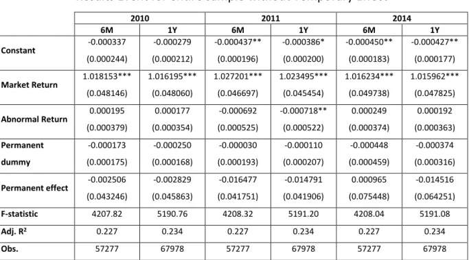
4.3 Results Event

The Results events (Table VI) demonstrate important differences in relation to

the other two events already analysed. The most relevant outcome is the absence

of abnormal returns associated with all the three European stress tests at any

range of data. This leads us to conclude that the results were already expected

and incorporated by the market participants in the bank’s shares prices. This

finding was already expected in this study since the investors have their own

methodologies. Also, after the official methodology release the market

participants can forecast the output results that will come few months after with

a good confidence interval.

4.4 The 2014 Stress Test

The tables VII and VIII compare the impact of 2014 tests between 2 groups –

the eight banks that failed the test against the others 33 banks in the entire

sample. This comparison is only done for 2014 stress test because this is the only

year with a significant sample for both groups.

As in the analysis with the entire sample, all regressions present a market daily

return coefficient statistically significant at 1% and a probability F-statistic equal

27

4.4.1 Banks above the minimum requirement

The banks which passed the 2014 test (Table VII) experienced a small positive

abnormal return of approximately 0.1% following the announcement date,

demonstrating that the market incorporated this press release believing the

banks were well prepared to pass the tests. In the Methodology and Results

events with 1 year data this group of banks had experienced a decline of their

permanent risk at 10% significance level of -0.10 on their beta share price,

revealing that their risk took in account the good results in this test.

4.4.2 Banks below the minimum requirement

In contrast, the banks who failed the test (Table VIII) had experienced a

negative abnormal return of 0.36% at 1% significance level after the Methodology

release and a positive abnormal return of 0.1% after the Results event. This show

us that the test impacted negatively the stock’s returns at the first moment but

after better results than expected led to an increase in stock’s returns.

The stock markets in the expectation of some banks to fail the test

incorporated previously the higher risk associated to these banks in the stocks’

price increasing their permanent risk (beta) on 0.37 since the first event.

In addition, this group had a temporary effect on its beta share price

28

overlapped with a permanent effect of 0.37 leaving us with an actual increase of

0.08 in the associated risk of those banks.

4.5 Additional Insights

In order to produce additional information and preventing distorted results

due to the overlapped dummies variables, we took the temporary dummy and its

interaction with the market from the regression.

The results are quite fascinating.

The sample of all banks considered in this dissertation and independently of

the amount of data used (Tables IX, X and XI) demonstrates a negative abnormal

return following the 2011 Methodology release and a positive abnormal return

after the 2014 Announcement event. Any regressions with this sample found the

statistically presence of a permanent effect on the beta share price for all the nine

events. This demonstrates that the banking system was poorly satisfied with 2011

Methodology confirming the empirical perception of that stress test and was

quite positive about the Announcement of 2014 stress test, derived from the

developments made.

In the comparison between the banks who failed and passed the 2014 stress

test (Tables XII and XIII) we observed a positive abnormal return above 1% in the

29

the test experienced this effect with the two range of data and the banks who

failed with only the 6 months’ range.

It was also detected an increase of permanent risk in all three events with 1

year data and only in the announcement event with 6 months’ data. In addition,

the Results event reduced the beta share price for the group of banks who passed

the test.

This is a strong evidence of the impact that these stress tests can provoke in

30

5. Conclusions

The main conclusions are that the Announcement event along with the

Methodology are the ones with a major impact on stock markets. That evidence

is namely shown in form of abnormal returns and not in terms of temporary or

permanent effect on banks’ risk. The Results event did not reveal any relevant

impact on the variables regarding the 3 European stress tests.

Yet the split of 2014 stress test in two groups shown an interesting different

impact of the test.

The group of banks that passed the test experienced a positive abnormal

return after the Announcement event and a decrease of their permanent risk

after the methodology and results event. In this case, the stress test was an

important and credible tool to inform the market about the security of these

banks.

The group of banks that did not achieve the minimum threshold was the

mostly impacted by the stock markets. They experienced a negative abnormal

return, first following the methodology event and a positive abnormal return

after the results release, giving the idea that the market was expecting worst

results. Although this group saw a decrease on its temporary risk followed by the

announcement, the permanent effect overrides the temporary leaving us with an

increase of the risk after all. This increase in risk was also experienced after the

31

processed the information given by the stress test and, as expected, penalized

the banks who failed the test increasing their risk and reducing their stock’s

returns.

In the overall, the begin of stress tests in 2010 were surrounded by distrust

and uncertainty. By not releasing the methodology used it contributed to increase

that feelings in the markets. After that, the methodology began to be released

and that was the key moment to the credibility of the EBA’s stress tests which

helped to gain some trust from the investors.

Since 2010 the stress tests improved a lot. At the beginning of the period

market focus seems to be concentrated on methodology’s fragility, in part, due

to its lack of maturity. With the course of time, improvements in the whole

process and a growing adherence to (actual or potential) loss events, the

attention of the markets turned to the specific potential bank’s results on the

stress tests.

We conclude that the stress tests are becoming relevant from year to year as

they become more realistic and giving real information to the markets, enabling

them to proceed with the necessary adjustments on their market valuations and

on stock’s risk.

Also, they helped to mitigate the risk in some cases, warning in other cases

32

EBA’s stress tests would be to increase the reality of the tests adding more

complexity to the simulation.

Nowadays, regulation is really becoming part of the system and can be one of

33

References

Alves, Mendes, V. and Silva, P., (2014). Do Stress Tests Matter? A Study on the

Impact of the Disclosure of Stress Test Results on European Financial Stocks and

CDS Markets. Portuguese Finance Network 2014.

Apergis, N. and Payne, J., (2013). European Banking Authority Stress Tests and

Bank Failure: Evidence from Credit Risk and Macroeconomic Factors. Banking and

Finance Review.

Bischof, J. and Daske, H., (2013). Mandatory Disclosure, Voluntary Disclosure, and

Stock Market Liquidity: Evidence from the EU Bank Stress Tests. Journal of

Accounting Research

Cardinali, A. and Nordmark, J., (2011). How informative are bank stress tests? -

Bank opacity in the European Union. Lund University.

Ellahie, A., (2013). Capital Market Consequences of EU Bank Stress Tests.

Research Paper.

Available at: https://a1papers.ssrn.com/sol3/papers.cfm?abstract_id=2157715

European Banking Authority (2010). EU-wide stress testing 2010

Available at:

https://www.eba.europa.eu/risk-analysis-and-data/eu-wide-stress-testing/2010

European Banking Authority (2011). EU-wide stress testing 2011

Available at:

34

European Banking Authority (2014). EU-wide stress testing 2014

Available at:

https://www.eba.europa.eu/risk-analysis-and-data/eu-wide-stress-testing/2014

Gick, W. and Pausch, T., (2012). Optimal Disclosure of Supervisory Information in

the Banking Sector.

Available at: https://a1papers.ssrn.com/sol3/papers.cfm?abstract_id=2006852

Jones, Lee, W. and Yeager, T. (2011). Opaque Banks, Price Discovery, and Financial

Instability. Journal of Financial Intermediation, Volume 21, Issue 3, July 2012,

Pages 383–408

Dowd, K. (2015). Central Bank Stress Tests: Mad, Bad, and Dangerous. Cato

Journal, Vol. 35, No. 3

Llorent, J., Melgar, M., Ordaz, J. and Guerrer, F., (2013). Stress Tests and Liquidity

Crisis in the Banking System. Quarterly Journal of Economics and Economic Policy,

Volume 8, Issue 2

Crisan, L., (2014). The stress test - A new challenge for the banking union.

International Journal of Business and Management Vol. II (4)

Nijskens, R. and Wagner, W., (2008). Credit Risk Transfer Activities and Systemic

Risk: How Banks Became Less Risky Individually But Posed Greater Risks to the

Financial System at the Same Time. Journal of Banking & Finance, Volume 35,

Issue 6, June 2011, Pages 1391–1398.

Neretina, Sahin, C. and de Haan, J., (2014). Banking Stress Test Effects on Returns

35

Peristian, Morgan, D. and Savino, V. (2010). The Information Value of the Stress

Test and Bank Opacity. FRB of New York Staff Report No. 460.

Petrella, G. and Resti, A., (2012). Supervisors as Information Producers: Do Stress

Tests Reduce Bank Opaqueness? Journal of Banking & FinanceVolume 37, Issue

36

Appendix

Table II Sample of Banks

Allied Irish Banks plc KBC Group NV Alpha Bank, SA Lloyds Banking Group plc Bank of Cyprus Public Company Ltd Banca Monte dei Paschi di Siena S.p.A.

Bank of Valetta plc National Bank of Greece, SA Bankinter SA Nordea Banck AB

Barclays plc OTP Bank Ltd Banco Bilbao Vizcaya Argentaria SA Piraeus Bank, SA

Banco Comercial Português, SA PKO Bank Polski

BNP Paribas Banco Popolare – Società Cooperativa Banco BPI, SA Banco Popular Español SA Commerzbank AG Royal Bank of Scotland plc Groupe Crédit Agricole Banco de Sabadell, SA

Danske Bank Banco Santander SA Deutsche Bank AG Svenska Handelsbanken AB

Dexia NV Société Générale

Erste Goup Bank AG Skandinaviska Enskilda Banken AB Eurobank Ergasias, SA Swedbank AB

HSBC Holdings plc Sydbank

ING Bank N.V. UBI

Intensa SanPaolo S.p.A. Unicredit S.p.A.

Jyske Bank -

Table III

Descriptive Statistics for all Samples

Entire Sample 2014 Failed banks 2014 Passed banks 6 months 1 year 6 months 1 year 6 months 1 year

Sample (Banks) 41 41 8 8 33 33

Sample (Share price) 57277 67978 11176 13264 46101 54714

Mean (Return %) -0.0469 -0.0413 -0.2368 -0.2313 -0.0008 0.0048

Median (Return %) 0 0 0 0 0 0

Std. Dev. (Return %) 3.4466 3.4759 5.7501 5.6307 2.6428 2.6575

Minimum (Return %) -45.0586 -45.0586 -45.0586 -45.0586 -43.8255 -43.8255

37 Table IV

Announcement Event for entire sample

2010 2011 2014

6M 1Y 6M 1Y 6M 1Y

Constant -0.000239 (0.000338) - 0.000226 (0.000219) -0.000496** (0.000227) -0.000402* (0.000220) -0.000564*** (0.000206) -0.000525*** (0.000199)

Market Return 1.019622***

(0.052596) 1.015052*** (0.051666) 1.024171*** (0.046449) 1.020604*** (0.046396) 1.011407*** (0.049936) 1.011473*** (0.048041) Abnormal Return 0.000400 (0.000507) 0.000404 (0.000528) -0.000796* (0.000458) -0.000797* (0.000456) 0.000968** (0.000399) 0.000976** (0.00098) Temporary dummy -0.000578** (0.000294) -0.000575** (0.000281) 0.000419** (0.000206) 0.000382* (0.000213) 0.000582** (0.000285) 0.000567** (0.000284) Temporary effect 0.016120 (0.029008) 0.019922 (0.027864) -0.055700* (0.029481) -0.052609 (0.034667) -0.029327 (0.042093) -0.013294 (0.047971) Permanent dummy -0.000223 (0.000261) -0.000261* (0.000155) -0.00000521 (0.000176) -0.000119 (0.000191) -0.0000405 (0.000188) -0.0000985 (0.000193) Permanent effect -0.007505 (0.036893) -0.005014 (0.047305) -0.006282 (0.041759) -0.005512 (0.043671) 0.047220 (0.059029) 0.016971 (0.058569)

F-statistic 2805.51 3460.84 2805.89 3461.09 2086.99 3461.63

Adj. R2 _{0.227 0.234 0.227 0.234 0.227 0.234}

Obs. 57277 67978 57277 67978 57277 67978

38 Table V

Methodology Event for entire sample

2010 2011 2014

6M 1Y 6M 1Y 6M 1Y

Constant -0.000357

(0.000307) -0.000281 (0.000210) -0.000321 (0.000203) -0.000288 (0.000205) -0.000495** (0.000197) -0.000465** (0.000191) Market Return 1.024748*** (0.052958) 1.017165*** (0.051800) 1.007791*** (0.047214) 1.009230*** (0.046110) 1.010662*** (0.049814) 1.010824*** (0.047943) Abnormal Return 0.000845 (0.000520) 0.000834* (0.000494) -0.000843** (0.000375) -0.000842** (0.000376) -0.001114** (0.000472) -0.001117** (0.000472) Temporary dummy -0.000346 (0.000285) -0.000374 (0.000244) 0.000172 (0.000361) 0.000165 (0.000356) 0.000786** (0.000388) 0.000773** (0.000368) Temporary effect 0.002926 (0.026933) 0.009346 (0.027497) 0.025145 (0.031462) 0.026816 (0.032171) 0.067763 (0.054728) 0.078742 (0.060767) Permanent dummy -0.000134 (0.000224) -0.000230 (0.000144) -0.000197 (0.000173) -0.000251 (0.000193) -0.000161 (0.000264) -0.000202 (0.000232) Permanent effect -0.011621 (0.041690) -0.006332 (0.049095) 0.007865 (0.042850) 0.003697 (0.043679) 0.031768 (0.065394) 0.006803 (0.061788)

F-statistic 2805.38 3460.69 2805.61 3460.92 2806.59 3461.64

Adj. R2 _{0.227 0.234 0.227 0.234 0.227 0.234}

Obs. 57277 67978 57277 67978 57277 67978

39 Table VI

Results Event for entire sample

2010 2011 2014

6M 1Y 6M 1Y 6M 1Y

Constant -0.000332

(0.000283) -0.000268 (0.000194) -0.000227 (0.000179) -0.000229 (0.000190) -0.000441** (0.000183) -0.000416** (0.000177)

Market Return 1.004848***

(0.051436) 1.009384*** (0.051320) 1.025209*** (0.047023) 1.021642*** (0.045274) 1.017872*** (0.049836) 1.016696*** (0.047709) Abnormal Return 0.000190 (0.000401) 0.000188 (0.000403) 0.001059 (0.000793) 0.001058 (0.000789) 0.000416 (0.000450) 0.000454 (0.000439) Temporary dummy 0.00000355 (0.000383) -0.0000179 (0.000303) -0.001873*** (0.000585) -0.001853*** (0.000578) -0.000243 (0.000331) -0.000316 (0.000276)

Temporary effect 0.0179201

(0.025989) 0.014762 (0.028670) 0.008535 (0.038021) 0.010806 (0.038141) -0.056572 (0.049237) -0.028115 (0.043033) Permanent dummy -0.000177 (0.000223) -0.000260* (0.000153) -0.000151 (0.000209) -0.000190 (0.000221) -0.000404 (0.000515) -0.000327 (0.000314)

Permanent effect 0.010034

(0.040137) 0.003416 (0.048727) -0.017491 (0.043485) -0.016029 (0.044163) 0.038181 (0.087669) -0.007858 (0.065480)

F-statistic 2805.20 3460.49 2808.22 3463.60 2085.74 3460.86

Adj. R2 _{0.227 0.234 0.227 0.234 0.227 0.234}

Obs. 57277 67978 57277 67978 57277 67978

40 Table VII

All Events for sample above the threshold in 2014

Announcement Methodology Results

6M 1Y 6M 1Y 6M 1Y

Constant -0.0000482

(0.000116) -0.0000446 (0.000128) -0.0000129 (0.000101) 0.00000386 (0.000111) -0.00000626 (0.0000959) -0.00000454 (0.000105)

Market Return 1.028789***

(0.059444) 1.029512*** (0.057405) 1.029201*** (0.059164) 1.030545*** (0.056809) 1.032064*** (0.058986) 1.031962*** (0.056678) Abnormal Return 0.000901** (0.000362) 0.000912** (0.000365) -0.000504 (0.000417) -0.000500 (0.000418) 0.000282 (0.000543) 0.000321 (0.000529) Temporary dummy 0.000135 (0.000225) 0.000113 (0.000220) 0.000142 (0.000337) 0.000119 (0.000304) 0.0000476 (0.000321) -0.0000339 (0.000278)

Temporary effect 0.033816

(0.034255) 0.053853 (0.039741) 0.058078 (0.045287) 0.034903 (0.059022) -0.037953 (0.046435) -0.009721 (0.041983) Permanent dummy -0.0000677 (0.000122) -0.0000419 (0.000131) -0.0000248 (0.000157) -0.000126 (0.000187) -0.000274 (0.000303) -0.000136 (0.000190)

Permanent effect -0.031443

(0.047596) -0.070379 (0.049566) -0.048734 (0.047698) -0.102483* (0.054129) -0.053877 (0.058419) -0.101373* (0.054193)

F-statistic 5142.18 6017.90 5142.47 6021.69 5143.68 6021.34

Adj. R2 _{0.40 0.40 0.40 0.40 0.40 0.40}

Obs. 46101 54714 46101 54714 46101 54714

41 Table VIII

All Events for sample below the threshold in 2014

Announcement Methodology Results

6M 1Y 6M 1Y 6M 1Y

Constant -0.002694***

(0.000432) -0.002507*** (0.000396) -0.002485*** (0.000484) -0.002325*** (0.000446) -0.002232*** (0.000472) -0.002114*** (0.000436)

Market Return 0.939707***

(0.067645) 0.937064*** (0.060732) 0.934186*** (0.068637) 0.932152*** (0.061735) 0.9593331*** (0.074185) 0.953725*** (0.067158) Abnormal Return 0.001244 (0.001389) 0.001238 (0.001375) -0.003634*** (0.001375) -0.003635*** (0.001377) 0.000968* (0.000502) 0.001001** (0.000488) Temporary dummy 0.002423*** (0.000861) 0.002440*** (0.000867) 0.003446*** (0.000958) 0.003391*** (0.000836) -0.001439 (0.000955) -0.001479** (0.000688)

Temporary effect -0.289789**

(0.126661) -0.290275** (0.147187) 0.107715 (0.208677) 0.104571 (0.225390) -0.133375 (0.161507) -0.103990 (0.133272) Permanent dummy 0.0000719 (0.000820) -0.000332 (0.000823) -0.000724 (0.001170) -0.000932 (0.000978) -0.000941 (0.002314) -0.001114 (0.001370)

Permanent effect 0.371707*

(0.191417) 0.377294** (0.167756) 0.363840 (0.237719) 0.374676** (0.190384) 0.417921 (0.348520) 0.377892* (0.198872)

F-statistic 156.54 208.53 156.31 208.36 154.88 206.83

Adj. R2 _{0.078 0.086 0.077 0.086 0.077 0.086}

Obs. 11176 13264 11176 13264 11176 13264

42 Table IX

Announcement Event for entire sample without Temporary Effect

2010 2011 2014

6M 1Y 6M 1Y 6M 1Y

Constant -0.000459

(0.000342) -0.000340 (0.000246) -0.000421* (0.000221) -0.000354 (0.000215) -0.000540*** (0.000201) -0.000504*** (0.000194)

Market Return 1.032515***

(0.050239) 1.024457*** (0.049773) 1.016838*** (0.047222) 1.015765*** (0.046489) 1.010886*** (0.049955) 1.011267*** (0.048135)

Abnormal Return -0.000061

(0.000453) -0.000107 (0.000404) -0.000501 (0.000373) -0.000521 (0.000363) 0.001473*** (0.000454) 0.001493*** (0.000461) Permanent dummy -0.000024 (0.000259) -0.000164 (0.000176) -0.000058 (0.000171) -0.000150 (0.000188) 0.000020 (0.000179) -0.000063 (0.000187)

Permanent effect -0.019456

(0.046084) -0.013342 (0.047792) -0.000859 (0.042132) -0.002270 (0.043411) 0.042659 (0.057341) 0.015905 (0.057313)

F-statistic 4207.99 5190.79 4207.88 5190.75 4210.11 5192.17

Adj. R2 _{0.227 0.234 0.227 0.234 0.227 0.234}

Obs. 57277 67978 57277 67978 57277 67978

Robust standard errors are in brackets. ***, ** and * signal the statistically significance at 1%, 5% and 10%, respectively.

Table X

Methodology Event for entire sample without temporary effect

2010 2011 2014

6M 1Y 6M 1Y 6M 1Y

Constant -0.000475 (0.000304) -0.000354 (0.000236) -0.000304 (0.000201) -0.000278 (0.000204) -0.000463** (0.000191) -0.000437** (0.000185)

Market Return 1.027747***

(0.049346) 1.022146*** (0.048969) 1.009771*** (0.047181) 1.010719*** (0.046170) 1.012136*** (0.049985) 1.012325*** (0.048119)

Abnormal Return 0.000572

(0.000472) 0.000534 (0.000431) -0.000722** (0.000312) -0.000727** (0.000309) -0.000362 (0.000281) -0.000346 (0.000288) Permanent dummy -0.000029 (0.000209) -0.000170 (0.000164) -0.000213 (0.000179) -0.000262 (0.000195) -0.000066 (0.000231) -0.000146 (0.000215)

Permanent effect -0.014422

(0.045893) -0.010815 (0.047537) 0.008674 (0.042494) 0.004864 (0.043315) 0.040290 (0.065938) 0.011633 (0.061898)

F-statistic 4208.09 5190.95 4208.25 5191.16 4208.59 5190.80

Adj. R2 _{0.227 0.234 0.227 0.234 0.227 0.234}

Obs. 57277 67978 57277 67978 57277 67978

43 Table XI

Results Event for entire sample without Temporary Effect

2010 2011 2014

6M 1Y 6M 1Y 6M 1Y

Constant -0.000337

(0.000244) -0.000279 (0.000212) -0.000437** (0.000196) -0.000386* (0.000200) -0.000450** (0.000183) -0.000427** (0.000177)

Market Return 1.018153***

(0.048146) 1.016195*** (0.048060) 1.027201*** (0.046697) 1.023495*** (0.045454) 1.016234*** (0.049738) 1.015962*** (0.047825) Abnormal Return 0.000195 (0.000379) 0.000177 (0.000354) -0.000692 (0.000525) -0.000718** (0.000522) 0.000249 (0.000374) 0.000192 (0.000363) Permanent dummy -0.000173 (0.000175) -0.000250 (0.000168) -0.000030 (0.000193) -0.000110 (0.000207) -0.000448 (0.000459) -0.000374 (0.000316)

Permanent effect -0.002506

(0.043246) -0.002829 (0.045863) -0.016477 (0.041751) -0.014791 (0.041906) 0.000965 (0.075448) -0.014516 (0.064251)

F-statistic 4207.82 5190.76 4208.32 5191.20 4208.04 5191.08

Adj. R2 _{0.227 0.234 0.227 0.234 0.227 0.234}

Obs. 57277 67978 57277 67978 57277 67978

Robust standard errors are in brackets. ***, ** and * signal the statistically significance at 1%, 5% and 10%, respectively.

Table XII

All Events for sample above the threshold in 2014 without temporary effect

Announcement Methodology Results

6M 1Y 6M 1Y 6M 1Y

Constant 0.0000421

(0.000110) -0.000040 (0.000122) -0.0000068 (0.0000962) -0.0000086 (0.000110) -0.00000450 (0.0000901) -0.00000568 (0.000101)

Market Return 1.029440***

(0.059346) 1.030421*** (0.057411) 1.030464*** (0.059181) 1.031291*** (0.057233) 1.030979*** (0.058601) 1.031712*** (0.056663)

Abnormal Return 0.001051**

(0.000447) 0.001062** (0.000454) -0.000333 (0.000253) -0.000327 (0.000258) 0.000337 (0.000374) 0.000298 (0.000357) Permanent dummy -0.0000567 (0.000116) -0.0000352 (0.000129) -0.0000172 (0.000134) -0.0000194 (0.000140) -0.000233 (0.000260) -0.000141 (0.000193)

Permanent effect -0.026715

(0.047298) -0.066407 (0.049013) -0.040821 (0.049918) -0.077773 (0.050875) -0.079447 (0.053200) -0.103693* (0.053294)

F-statistic 7713.11 9025.97 7712.65 9027.14 7715.19 9032.28

Adj. R2 _{0.40 0.398 0.40 0.398 0.40 0.398}

Obs. 46101 54714 46101 54714 46101 54714

44 Table XIII

All Events for sample below the threshold in 2014 without temporary effect

Announcement Methodology Results

6M 1Y 6M 1Y 6M 1Y

Constant -0.002593***

(0.000450) -0.002417*** (0.000557) -0.002344*** (0.000498) -0.002202*** (0.000454) -0.002287*** (0.000461) -0.002164*** (0.000425)

Market Return 0.934351***

(0.068632) 0.932261*** (0.030690) 0.936533*** (0.071724) 0.934091*** (0.064277) 0.955410*** (0.077298) 0.950995*** (0.069201) Abnormal Return 0.003212*** (0.001244) 0.003273 (0.002939) -0.000480 (0.000990) -0.000427 (0.001021) -0.000115 (0.001123) -0.000246 (0.001119) Permanent dummy 0.000338 (0.000772) -0.000175 (0.001030) -0.000269 (0.001044) -0.000666 (0.000914) -0.001334 (0.002063) -0.001333 (0.001360)

Permanent effect 0.328827*

(0.188651) 0.355445*** (0.083959) 0.374871 (0.233305) 0.380429** (0.188358) 0.332667 (0.290340) 0.353338* (0.197727)

F-statistic 233.80 311.68 233.76 311.78 232.07 309.99

Adj. R2 _{0.077 0.086 0.077 0.086 0.076 0.085}

Obs. 11176 13264 11176 13264 11176 13264