Counterparty and Liquidity Risk: an analysis of the negative basis

(1)

ISEG – Instituto Superior de Economia e Gestão

Master in Finance

Masters Final Assignment

Year: 2010 / 2011

PROJECT

Counterparty and Liquidity Risk: an analysis of the negative basis

Vladimir João de Oliveira Lopes Dias da Fonseca

Supervision: Raquel M. Gaspar

(2)

Abstract

In this study we analyse the equivalence between credit default swap (CDS) spreads and corporate bond yield spreads from March 2007 to March 2011 for investment graded corporate entities in the eurozone. We find evidence of cointegration between the two markets and that CDS prices tends to lead corporate yield spreads. We find support for significant effects of counterparty and funding risks in the basis, measured as the difference between CDS and corporate yield spreads, with negative impact, and that liquidity also matters in this context.

(3)

Resumo

No contexto da relação teórica de equilíbrio entre os preços dos CDS e as yield spreads

das obrigações das empresas face a taxas de juro sem risco, este trabalho conclui que existe cointegração entre estas duas variáveis para entidades de referência na zona euro no período que decorre entre Março de 2007 e Março de 2011. A análise efectuada revelou que o risco de contraparte e o risco de liquidez em ambos os mercados tiveram um impacto significativo na base, entre os CDS e os referidos spreads, e que os preços dos CDS tenderam a liderar as yield spreads das obrigações no período em análise.

(4)

Acknowledgments

(5)

List of Tables

Table 1 - Basket of France Telecom bonds for the corporate yield spread calculation ... 7

Table 2 - Bond spread and credit spread computation procedure ... 8

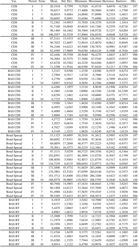
Table 3 - Descriptive Statistics... 13

Table 4 - Unit root testing ... 16

Table 5 - Stationarity testing ... 17

Table 6 - Estimated potentially cointegrating equations and residual tests for France Telecom 18 Table 7 - Estimated error correction model for France Telecom ... 19

Table 8 - Regression of basis spreads on counterparty and funding risks, liquidity and broad market conditions proxies for France Telecom ... 24

Table 9 - Dataset summary... 26

Table 10 - Average spreads of main variables for 5 year maturity ... 27

Table 11 - Cointegration analysis and Lead-Lag relationship between CDS and bond markets for the reference entities in analysis ... 29

(6)

List of Figures

Figure 1 - Time series plot of France Telecom CDS premium mid quotations at 3, 5, 7 and 10

years maturity... 6

Figure 2 - Computed yields on equivalent riskless bonds... 9

Figure 3 - Individual bond spreads (ECB yield curve as benchmark) for each France Telecom selected bonds, from March 2007 to March 2011... 10

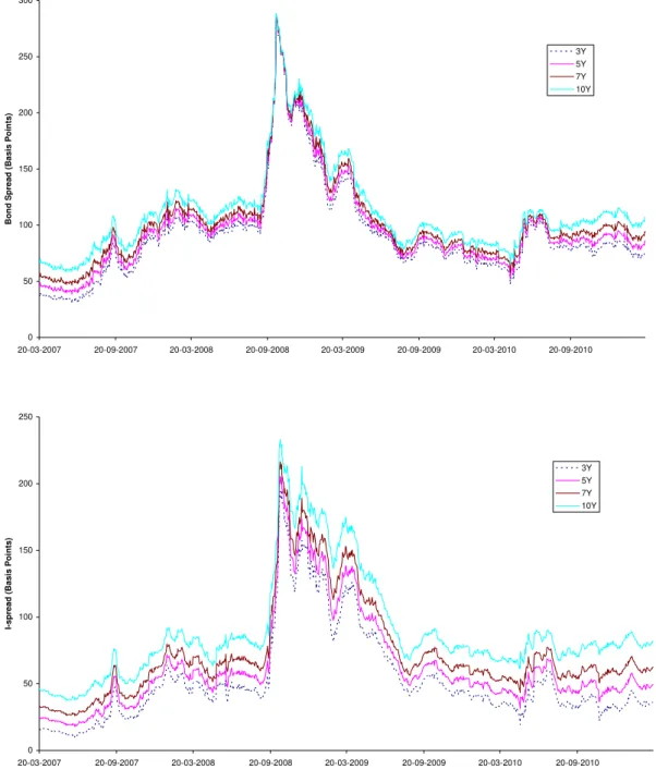
Figure 4 - Corporate spread measures, bond spread on top and i-spread bellow, for France Telecom from March 2007 to March 2011 ... 11

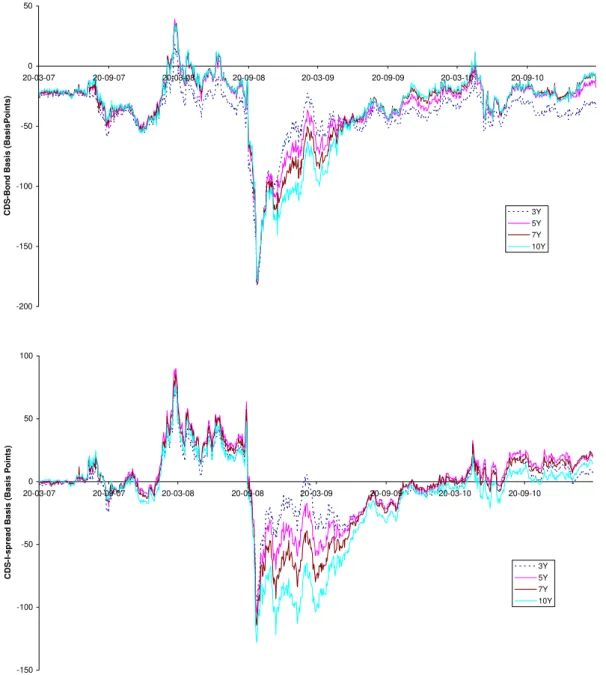
Figure 5 - Corporate basis measures, CDS-Bond basis on top and CDS-i-Spread basis bellow, for France Telecom from March 2007 to March 2011... 12

Figure 6 - Euribor-EONIA spread evolution in 2007-2011 period ... 22

Figure 7 - Bid-Ask spreads for France Telecom CDS (on top) and bond yields (bellow) ... 23

(7)

Chapter 1 Introduction

IN THE PAST SEVERAL YEARS, the importance of credit derivative markets has been growing rapidly. The single most important instrument in this market is the credit default swap (CDS). A CDS is a bilateral agreement to exchange the credit risk of a reference entity. In this agreement, one party (the protection buyer) pays a periodic fee (CDS premium) to another party (the protection seller) in exchange for compensation in case of a credit event (bankruptcy, failure to pay, default, restructuring, repudiation or moratorium, among others) of a given reference entity. In theory, this CDS premium is expected to reflect the perceived credit risk of the reference entity in a pure way.

Therefore, these CDS contracts provides a new way to measure the size of the default component in corporate spreads and many authors argue that an arbitrage relationship exists between CDS prices and corporate yield spreads for a given reference entity, as first discussed by Duffie (1999)1 and then pointed out by Blanco, Brennan et al. (2005) in their empirical analysis of the dynamic relations between bond and CDS markets.

Blanco, Brennan et al. (2005) argue that if an investor buys a T year par bond with yield to maturity y and at the same time buys credit protection in CDS market on the same reference entity for T years at a cost of pCDS (annually), she has eliminated most of the

default risk associated with the bond at an annual return of y - pCDS. By arbitrage, this

net return should be approximately equal to the T year risk free rate, x. For example, if y - pCDS is less than x, then shorting the bond, selling protection in CDS market and

buying the risk free instrument would be a profitable arbitrage opportunity2.

In this context, an equilibrium theoretical condition is expected to hold in the long run between the corporate yield spreads and the CDS prices, even though, significant deviations are documented in many empirical studies, especially in the short term.

Why this basis, between CDS prices and corporate yield spreads, deviates from zero? If in one hand, a liquidity premium may be included in the corporate yield spreads, driving this basis negative, in the other hand, other factors affecting the CDS premium also contribute to obscure this relationship, namely the counterparty risk (as CDS are OTC

1

Duffie (1999) has demonstrated that the CDS price should be equal to the spread between a par risky floating rate note over a risk free floating rate note.

2

Likewise, the same authors explain that, if y - pCDS is more than x, buying the bond, buying protection in

(9)

products, this risk tend to lower the CDS premium because protection buyers face greater uncertainty in receiving the asset value should the default occur, and therefore are only willing to pay a lower premium as agued by De Wit (2006)) and the liquidity risk of the CDS itself, which would tend to turn the basis positive.

The notion that liquidity is priced in corporate yield spreads started with Amihud and Mendelson (1986). They studied the effect of bid-ask spreads in asset pricing and returns. Among other relevant articles, Ericsson and Renault (2006) provides a comprehensive insight on the impact of the liquidity risk in the corporate yield spreads, developing a structural model that simultaneously captures liquidity and credit risk. This study documents positive correlation between illiquidity and default component and supports a downward-sloping term structure for liquidity spreads. Chen, Lesmond et al. (2007) provides an extensive analysis on how “more illiquid bonds earn higher yield spreads” using several liquidity measures and covering more than 4,000 corporate bonds, over different categories.

The recent financial crisis has stressed out the importance of the liquidity risk in the financial markets. In this period, the CDS premium has experienced a tremendous increase, as much as many studies documented the basis (between CDS and corporate yield spreads) to be strongly negative. This fact sparked new questions about the possibility of CDS prices to include significant risks other then credit risk, namely the counterparty and CDS own liquidity as stated before, not pricing correctly the reference entity default risk, which also has increased tremendously in this period with great impact in the corporate bond yields.

In this context, the present study proposes, under the non-arbitrage condition above discussed, an empirical assessment in to what extend the equilibrium between the CDS prices and the corporate yield spreads has hold in the last few years and what were the determinants of the basis spread changes for corporate investment graded reference entities in the eurozone, including the role of counterparty and liquidity risk.

(10)

Chapter 2 Conceptual Framework

At this point, it is useful to clarify some of the concepts and terminology that will be used throughout this text. The CDS premium (or sometimes referred to as CDS price, or CDS spread, or just CDS) is the premium paid by the protection buyer to the protection seller, quoted in basis points per annum (usually paid quarterly) and it is a very straightforward measure that tends to reflect the credit risk of a given reference entity.

However, different concepts of corporate yield spreads exist, depending on the riskless benchmark choice and the calculation procedures. For the purpose of this study, the term bond spread will be used to denote the difference between the yield on a corporate bond and the yield on a riskless bond with identical promised cash flows, as defined in Longstaff, Mithal et al. (2005), with the riskless benchmark being the European Central Bank (ECB) spot yield curve3.

A second approach to the corporate yield spread will also be used as alternative to the bond spread above defined, as many authors, including Blanco, Brennan et al. (2005), now argue that government bonds are no longer the ideal proxy for the risk free rate, naming factors like taxation treatment, repo specialness, scarcity premium, impacting its behaviour. Also, Longstaff, Mithal et al. (2005) use three different alternatives of risk-free rate to generate their riskless discount function in order to robust check their findings.

Therefore an alternative proxy of the risk-free rate, very much used nowadays, is the interest rate swap curve, although some may argue that swaps contain a credit premium because there is some counterparty risk. The differential between the yield on a corporate bond and interpolated swap rates4 is called i-spread and will be used as an alternative measure of corporate yield spread and be denoted as i-spread.

Both spread measures above will be expressed in basis points per annum, in order to compare with the CDS spread, originating two more measures: the CDS-bond basis, as the difference between the CDS spread and the bond spread (using government bonds as

3

This (spot) yield curve is estimated from a sample of “AAA-rated” euro area central government bonds, using the Svensson model. The selection criteria and additional information are available in the ECB website.

4

(11)

the benchmark) and the CDS-i-spread basis as the differential between the CDS spread and the i-spread (using the swap curve as the benchmark).

With the purpose to access (1) the equilibrium condition between the CDS prices and the corporate yield spreads and (2) the determinants of the basis spread changes, and considering that the data to be processed will consist in time series observations for each variable, it is necessary to evaluate and select an appropriate estimation method. The fist approach would be to use a standard ordinary least square (OLS) method to estimate a regression model with selected explanatory variables but, since the use of non stationary variables can lead to spurious regression the evaluation of that condition and the estimation model to be applied will have to take this into consideration.

A stationary series can be defined as one with a constant mean, constant variance and constant autocovariances for each given lag, Brooks (2008). For a stationary series, the “shocks” will gradually die away and the series will cross its mean value frequently. In a non stationary series, shocks to the system will persist in time and the series can drift long time away form their mean, which they cross rarely.

A standard way to cope with this problem (of regressing non stationary variables) is to differentiate the series instead of using the levels. If a non stationary series have to be differentiated one time before becoming stationary it is said to contain one unit root, or to be integrated of order one, I(1). If it has to be differentiated d times before it becomes stationary, it is said to be integrated of order d, I(d).

Still according to Brooks (2008), most financial time series contains one unit root, so testing this hypotheses will be the first step before any estimation procedure5. For the purpose of this study, and among others available methods, the augmented Dickey-Fuller test6 (ADF test) will be used for unit root testing and, in other to test the robustness of the results, the KPSS7 test, Kwiatkowski, Phillips et al. (1992), will be performed, following the confirmatory data analysis proposed in Brooks (2008).

In order to evaluate the equilibrium condition between CDS and bond markets, an error correction model will be used. Considering that pure first difference models have no

5

This is an important issue as differentiating more than necessary to achieve stationarity will introduce an MA (moving average) structure to the errors, and not differentiating enough times will still lead to a non stationary series, both undesirable situations.

6

Developed by Fuller (1976) and Dickey and Fuller (1979), this test has unit root under the null hypothesis.

7

(12)

long term solution8, error correction models (or equilibrium correction models) can overcome the non stationarity issue by combining first differences and lagged levels of cointegrated9 variables. These models are in the base of the modelling strategy called the Engle-Granger 2-step method, in which, using a residual based approach, in the first step, a cointegrating equation is estimated.

If a cointegrating relationship is found in step 1, the appropriate modelling strategy in this framework is to use this stationary linear combination of the variables in hand in a general equilibrium model for the analysis. If not, the appropriate strategy for econometric modelling would be than to use first differences specifications only. This strategy will be detailed in the next section case study of France Telecom to analyse cointegration and lead-lag relationship between CDS and bond markets.

8

As pointed out in Brooks (2008) , if we consider two series yt and xt, both I(1), the model one may

consider estimating is Δyt = βΔxt + εt. For the model to have a long run solution, the variables must

converge to some long term value and so, no longer changing, meaning yt = yt-1 = y and xt = xt-1 = x, i.e.

Δy = 0 and Δx = 0, cancelling everything in the equation. Therefore this model has little to say about any equilibrium condition between yt and xt.

9

(13)

Chapter 3 Methodology Illustration: France Telecom Case Study

In order to address the investigation problem in hand, it is useful to illustrate first the above discussed methodology via a case study, France Telecom, during the period from 2007, i.e. before the 2008 financial crisis, to the present (March 2011). This timeframe comprises both pre-crisis and post-crisis scenarios, as well as the great financial markets turmoil period of 2008.

3.1 The Basis

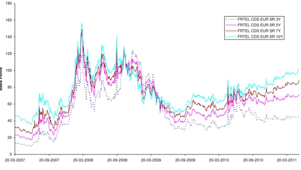
The CDS data consists of daily mid, bid and ask quotations for credit default swaps on senior France Telecom debt, with maturities of 3, 5, 7 and 10 years, obtained from Bloomberg financial terminal covering the period from March 2007 to March 2011. Figure 1 plots the evolution of the CDS spreads over the analysis period. As shown, the premium increases with the maturity in most of the time, as expected, and an enormous enlargement occurred during the 2008 crisis period from around 20 basis points in the 5 year tenor to more than 100 basis points. The after crisis period, in 2009, is characterized by a steady upward trend in all maturities, except for the 3 year tenor, after the decrease from the extremely high 2008 values.

Figure 1 - Time series plot of France Telecom CDS premium mid quotations at 3, 5, 7 and 10 years maturity

0 20 40 60 80 100 120 140 160 180

20-03-2007 20-09-2007 20-03-2008 20-09-2008 20-03-2009 20-09-2009 20-03-2010 20-09-2010 20-03-2011

Basis P

o

in

ts

(14)

Since all the CDS in the sample have constant maturities, the problem now is to find the appropriate corporate spread measure to compare with. While it is not possible to always find a bond with an exact maturity to match with the CDS premium, and then compare the spreads, it is necessary to find an appropriate approach to this maturity matching problem. Many approaches are available in the related literature, including Gaspar and Pereira (2010), but in this regard, a quite robust one is presented in Longstaff, Mithal et al. (2005). Rather then focusing in a specific bond to compute the corporate yield spread, those authors prefer to apply a disjoint method, in which they propose to select a basket of bonds with maturities that bracket the desired horizon (5 year in their case) to compute the corporate yield spread.

To compute the corporate yield spread, they use the following procedure: for each bond in the basket set, they solve for the yield on a riskless bond with the same maturity and coupon rate, using three different riskless benchmark curves. Subtracting this riskless yield to the respective corporate bond yield, they find the yield spread for that particular bond. To obtain the desired 5-year maturity, they regress the yield spreads obtained for each bond in the basket set on their maturity and use fitted value at 5-year as the estimate for the corporate yield spread. They also present in the appendix B of their paper a very useful list of criteria for the bonds selection process.

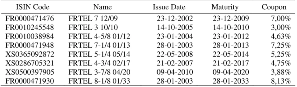
Following this procedure, a set of eight bonds were selected for the France Telecom case study, with maturities ranging from less than 3-years to 25-years, to cover all maturities in analysis and with a “term structure” the most homogeneous as possible. The bond selection criteria included only large issued senior debt, denominated in euro and with fixed coupon rate.

Table 1 - Basket of France Telecom bonds for the corporate yield spread calculation

ISIN Code Name Issue Date Maturity Coupon

FR0000471476 FRTEL 7 12/09 23-12-2002 23-12-2009 7,00%

FR0010245548 FRTEL 3 10/10 14-10-2005 14-10-2010 3,00%

FR0010038984 FRTEL 4-5/8 01/12 23-01-2004 23-01-2012 4,63%

FR0000471948 FRTEL 7-1/4 01/13 28-01-2003 28-01-2013 7,25%

XS0365092872 FRTEL 5-1/4 05/14 22-05-2008 22-05-2014 5,25%

XS0286705321 FRTEL 4-3/4 02/17 21-02-2007 21-02-2017 4,75%

XS0500397905 FRTEL 3-7/8 04/20 09-04-2010 09-04-2020 3,88%

FR0000471930 FRTEL 8-1/8 01/33 28-01-2003 28-01-2033 8,13%

(15)

Full description of the bonds, including ISIN code, name, coupon rate, maturity, rating and daily series of bid, ask and mid quotations for prices and yields to maturity were obtained from a from a Bloomberg financial terminal covering the period in analysis. The ECB yield curve is based in the Svensson model and the spot rate, z, for any desired maturity can be obtained using the following equation:

⎥ ⎥ ⎥ ⎥ ⎥ ⎦ ⎤ ⎢ ⎢ ⎢ ⎢ ⎢ ⎣ ⎡ − ⎟⎟ ⎠ ⎞ ⎜⎜ ⎝ ⎛ − + ⎥ ⎥ ⎥ ⎥ ⎥ ⎦ ⎤ ⎢ ⎢ ⎢ ⎢ ⎢ ⎣ ⎡ − ⎟⎟ ⎠ ⎞ ⎜⎜ ⎝ ⎛ − + ⎥ ⎥ ⎥ ⎥ ⎥ ⎦ ⎤ ⎢ ⎢ ⎢ ⎢ ⎢ ⎣ ⎡ ⎟⎟ ⎠ ⎞ ⎜⎜ ⎝ ⎛ − + = ⎟⎟⎠ ⎞ ⎜⎜ ⎝ ⎛ − ⎟⎟ ⎠ ⎞ ⎜⎜ ⎝ ⎛ − ⎟⎟ ⎠ ⎞ ⎜⎜ ⎝ ⎛ − ⎟⎟ ⎠ ⎞ ⎜⎜ ⎝ ⎛ − ⎟⎟ ⎠ ⎞ ⎜⎜ ⎝ ⎛ − 2 2 1 1 1 2 3 1 2 1 1 0 1 1 1 ) ( τ τ τ τ τ τ β τ β τ β β TTM TTM TTM TTM TTM e TTM e e TTM e TTM e TTM z ₍₁₎

Where TTM is the term to maturity and βi and τi are the model parameters to be

estimated. The ECB provides daily series for the parameters above, so daily discount factors for our riskless bond with the same maturity and coupon rate can be computed. In this case, for each bond in the basket set and in a daily basis, an identical bond with the same promised cash flows was considered and each cash flow was discounted at its own riskless rate to obtain the riskless yield for that particular bond.

For the alternative measure, i-spread, the difference between the yield to maturity of each bond in the basket set and the interpolated swap rate was computed. Table 2 details the calculations for the first bond of France Telecom case study in reference to the 20th of March 2007 (the first day of the analysis period).

Table 2 - Bond spread and credit spread computation procedure

This table reports the computation procedure for bond spread and i-spread measures for the

bond FR0000471476 FRTEL 7 12/09. For each day in the sample, the 20th of March 2007

in this example, the Svensson model parameters for the AAA-rated eurozone government bonds yield curve were retrieved from the ECB in order to compute the discount factors to apply to the promised cash flows of an equivalent bond and to determine its theoretical risk free price and then its yield (yRF, that was 3,93% in this case). The SWAP interest rates

were downloaded from Bloomberg financial terminal, and interpolated for the maturity of the bond in analysis in the 20th of March 2007, 2,76 years. The basis were computed as the respective differences in basis points to the bond yield to maturity in that date, 4,36%.

Date: 20-03-2007

ECB Svensson Model Parameters Swap Interest Rate

β0 4,2429 2-years 4,1545

β1 -0,7780 3-years 4,1265

β2 0,3560

β3 -1,3269

τ1 0,4377

τ2 3,0657

Bond Price: 101,1410

(16)

Table 2 (Continued)

23-12-2007 23-12-2008 23-12-2009

Cash Flows 7% 7% 107%

TTM (D) 278 644 1009

TTM (Y) 0,7616 1,7596 2,7644

z(TTM)=r(t,T) 3,8405 3,8712 3,8398

B(t,T) (discount factors) 0,9712 0,9342 0,8993

Gross PriceRF Settl. Date Int. Accr. Date Accr. Int. Clean PriceRF

109,5615 23-03-2007 23-12-2006 1,7260 107,8355

yRF (%) 3,9322 Bond Spread (bp) 33,4655

i-swap rate (%) 4,1331 I-Spread (bp) 13,3719

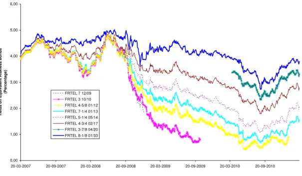
The above procedure was repeated for the remaining bonds in the basket set and for the period in analysis. Figure 2 pictures the evolution of the riskless yield obtained for each bond in the set. As expected the riskless bonds with high maturity presented higher yields during most of the period, especially after the 2008 period. It is remarkable the flattening of the yields that has occurred in June 2008, few months before the Lehman Brothers collapse and great turmoil in financial markets. The short term interest rates were very high.

Figure 2 - Computed yields on equivalent riskless bonds

The pre-crisis period was characterized by the flattening of the yield curve, namely in June 2008.

0,00 1,00 2,00 3,00 4,00 5,00 6,00

20-03-2007 20-09-2007 20-03-2008 20-09-2008 20-03-2009 20-09-2009 20-03-2010 20-09-2010

Y

ie

lds o

n

E

quiv

a

lent

R

iskless Bo

nds

(P

er

cen

tage

)

FRTEL 7 12/09 FRTEL 3 10/10 FRTEL 4-5/8 01/12 FRTEL 7-1/4 01/13 FRTEL 5-1/4 05/14 FRTEL 4-3/4 02/17 FRTEL 3-7/8 04/20 FRTEL 8-1/8 01/33

(17)

At this point, after some intervention of the authorities lowering the short term interest rates, the shape of the yield curves began to normalize.

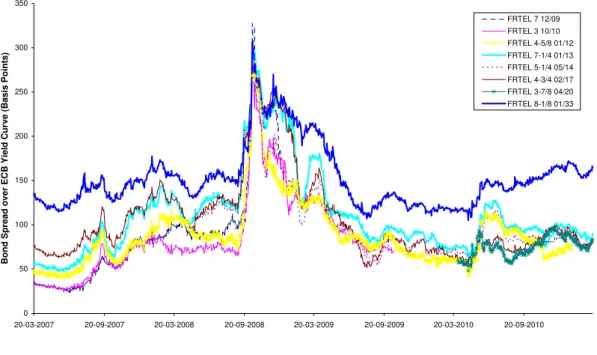
Following Longstaff, Mithal et al. (2005) procedure, Figure 3 presents the corporate yield spread over ECB spot yield curve obtained for each France Telecom bond in the set for the period in analysis. These spreads contained the desired maturities of the CDS.

Figure 3 - Individual bond spreads (ECB yield curve as benchmark) for each France Telecom selected bonds, from March 2007 to March 2011.

0 50 100 150 200 250 300 350

20-03-2007 20-09-2007 20-03-2008 20-09-2008 20-03-2009 20-09-2009 20-03-2010 20-09-2010

Bo

nd

S

p

re

ad

over

E

C

B Y

ield

Cur

ve (Basi

s P

o

ints)

FRTEL 7 12/09 FRTEL 3 10/10 FRTEL 4-5/8 01/12 FRTEL 7-1/4 01/13 FRTEL 5-1/4 05/14 FRTEL 4-3/4 02/17 FRTEL 3-7/8 04/20 FRTEL 8-1/8 01/33

(18)

Figure 4 - Corporate spread measures, bond spread on top and i-spread bellow, for France Telecom from March 2007 to March 2011

0 50 100 150 200 250 300

20-03-2007 20-09-2007 20-03-2008 20-09-2008 20-03-2009 20-09-2009 20-03-2010 20-09-2010

Bon

d

S

p

read (

B

asis P

o

in

ts)

3Y 5Y 7Y 10Y

0 50 100 150 200 250

20-03-2007 20-09-2007 20-03-2008 20-09-2008 20-03-2009 20-09-2009 20-03-2010 20-09-2010

I-spr

ead

(Basis P

o

in

ts)

3Y 5Y 7Y 10Y

(19)

Figure 5 - Corporate basis measures, CDS-Bond basis on top and CDS-i-Spread basis bellow, for France Telecom from March 2007 to March 2011

-200 -150 -100 -50 0 50

20-03-07 20-09-07 20-03-08 20-09-08 20-03-09 20-09-09 20-03-10 20-09-10

CD

S

-B

o

n

d

Bas

is

(B

a

s

is

P

o

in

ts

)

3Y 5Y 7Y 10Y

-150 -100 -50 0 50 100

20-03-07 20-09-07 20-03-08 20-09-08 20-03-09 20-09-09 20-03-10 20-09-10

CD

S

-I-sp

re

a

d

B

a

sis (Bas

is P

o

in

ts

)

3Y 5Y 7Y 10Y

(20)

It is possible then to split the analysis period in four, a pre crisis period in 2007 (up to the end of the year), a crisis period before Lehman Brothers collapse and another after this event in September 2008 and a post crisis period with the markets recovery that began in March 2009. Table 3 presents descriptive statistics for the above discussed variables obtained for France Telecom.

Table 3 - Descriptive Statistics

(21)

Table 3 (continued)

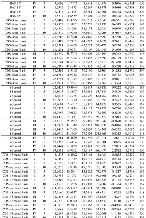
BAS BY IV 3 9,3608 2,7752 3,9648 15,4879 0,3996 -0,8301 506 BAS BY IV 5 8,5542 2,4373 4,2267 13,9471 0,4656 -0,7598 506 BAS BY IV 7 7,7476 2,1105 3,8762 12,4701 0,5372 -0,6531 506 BAS BY IV 10 6,5377 1,6559 3,3504 10,4753 0,6408 -0,4524 506 CDS-Bond Basis I 3 -32,9407 11,4245 -59,0772 -17,5645 -0,6531 -0,9349 197 CDS-Bond Basis I 5 -29,9575 10,3162 -52,7770 -11,8185 -0,6348 -0,8171 197 CDS-Bond Basis I 7 -29,4840 10,3266 -54,7175 -12,3080 -0,6999 -0,5802 197 CDS-Bond Basis I 10 -28,4319 10,9260 -56,1031 -7,2968 -0,7667 -0,1649 197 CDS-Bond Basis II 3 -25,0766 12,7240 -49,4040 17,9999 0,7230 1,3384 167 CDS-Bond Basis II 5 -11,1482 16,2165 -44,9282 39,0674 0,2621 0,8488 167 CDS-Bond Basis II 7 -10,2581 16,4460 -45,5235 35,6476 0,0230 0,5208 167 CDS-Bond Basis II 10 -10,4281 17,0571 -49,7109 34,1647 -0,1696 0,4193 167 CDS-Bond Basis III 3 -74,0749 38,7744 -181,9206 -22,4193 -0,9362 0,2602 148 CDS-Bond Basis III 5 -79,6149 35,7294 -181,5497 -12,5599 -0,6199 0,5300 148 CDS-Bond Basis III 7 -87,1544 34,3803 -180,6653 -10,7718 -0,1420 0,6437 148 CDS-Bond Basis III 10 -96,3989 34,4348 -179,3332 -9,5043 0,5220 0,8322 148 CDS-Bond Basis IV 3 -38,3502 8,3108 -59,2190 -6,0300 0,1832 0,1839 506 CDS-Bond Basis IV 5 -29,8784 11,9332 -69,8379 6,4446 -0,5433 0,4095 506 CDS-Bond Basis IV 7 -27,6751 14,1999 -80,9007 10,7972 -0,9871 1,4808 506 CDS-Bond Basis IV 10 -27,9971 16,2682 -90,5962 12,4362 -1,3354 2,5830 506 i-Spread I 3 22,6453 10,4684 9,8413 48,0182 0,9222 -0,2068 197 i-Spread I 5 30,8013 10,5107 17,9056 55,7649 0,8800 -0,2616 197 i-Spread I 7 38,9574 10,5785 25,9699 63,8259 0,8311 -0,3228 197 i-Spread I 10 51,1915 10,7270 37,6362 76,3656 0,7492 -0,4244 197 i-Spread II 3 47,8684 5,6237 35,2871 64,0272 0,3525 0,2445 167 i-Spread II 5 57,2325 5,5156 43,3122 71,9282 0,0710 0,2982 167 i-Spread II 7 66,5967 5,6125 51,3374 79,8292 -0,2800 0,3724 167 i-Spread II 10 80,6430 6,1151 63,3751 92,3579 -0,7043 0,4217 167 i-Spread III 3 120,6170 35,5567 39,2980 195,2847 -0,3670 0,0117 148 i-Spread III 5 133,7812 35,1049 50,2817 205,3036 -0,4936 0,1779 148 i-Spread III 7 146,9455 34,7400 61,2653 216,4207 -0,6272 0,3693 148 i-Spread III 10 166,6919 34,3609 77,7408 233,0963 -0,8343 0,6942 148 i-Spread IV 3 46,8261 18,4879 19,2293 126,3211 1,8631 3,7007 506 i-Spread IV 5 57,4353 18,4164 31,2591 138,2601 2,0655 4,4044 506 i-Spread IV 7 68,0444 18,5138 43,2889 150,1990 2,2065 4,9304 506 i-Spread IV 10 83,9582 18,9702 61,3189 168,1074 2,2882 5,2772 506 CDS-i-Spread Basis I 3 -2,4535 6,2092 -24,5164 14,8086 -0,8025 2,2427 197 CDS-i-Spread Basis I 5 -0,1497 6,4459 -19,6141 21,0218 0,3412 1,4373 197 CDS-i-Spread Basis I 7 -0,3555 6,4133 -16,1118 21,0976 0,3632 1,2329 197 CDS-i-Spread Basis I 10 -0,3223 7,8016 -17,5716 25,1500 0,3360 1,1419 197 CDS-i-Spread Basis II 3 24,3682 16,2641 -12,1822 73,2778 0,1847 1,1738 167 CDS-i-Spread Basis II 5 34,4783 19,1973 -9,3846 90,0461 -0,0315 1,0274 167 CDS-i-Spread Basis II 7 31,5502 18,8023 -12,6698 85,3723 -0,1173 0,8735 167 CDS-i-Spread Basis II 10 25,6528 18,3556 -17,2900 76,4087 -0,1324 0,8156 167 CDS-i-Spread Basis III 3 -23,3028 26,3342 -94,7673 52,1188 -0,0930 1,2535 148 CDS-i-Spread Basis III 5 -37,0160 30,9157 -105,2046 63,6214 1,0262 1,6218 148 CDS-i-Spread Basis III 7 -52,7288 34,2627 -114,4307 57,6139 1,4227 1,7707 148 CDS-i-Spread Basis III 10 -74,2330 39,0970 -128,2483 47,6533 1,6140 1,7395 148 CDS-i-Spread Basis IV 3 -4,3815 15,2003 -38,8567 27,3837 -0,4956 -0,6435 506 CDS-i-Spread Basis IV 5 -1,1668 19,5958 -55,7566 32,8559 -0,7384 -0,2973 506 CDS-i-Spread Basis IV 7 -4,2207 21,4726 -71,7360 30,2061 -1,1180 0,6374 506 CDS-i-Spread Basis IV 10 -12,4285 23,2986 -90,8504 21,3415 -1,4472 1,6094 506

In the period I, the CDS premium and the bond spreads were relatively low and the basis measures were at their equilibrium point. The CDS-i-spread basis was near zero, suggesting that the theoretical non arbitrage condition was holding relatively well during this period. The CDS-bond basis was 30bp negative, but this difference may be related to liquidity and other factors as above discussed.

(22)

to occur in the CDS market, that leads to some extend corporate spreads in the short term. As a result, the basis, measured with swap benchmark turned into positive territory. Other possible factors that could drive the basis positive is discussed by De Wit (2006), and may include CDS cheapest to deliver option, as in case of default, protection buyers hold a delivery option and are free to choose the cheapest from a basket of deliverable bonds. Protection sellers will tend receive the less favourable option and therefore to increase the CDS premium if this risk increases. He also appoints other factors like bonds trading bellow par and profit realization among others.

Period III documents a large increase in the corporate yield spread measures reflecting in parte the great increase of the default risk that occurred in this period, after the Lehman Brothers collapsed. The level of CDS spreads were not increasing as much as the corporate spreads and the basis became highly negative. Some authors, like De Wit (2006), could argue that the CDS premium was reflecting some of the high counterparty risk that CDS market was experiencing in that period, when banks were not lending to each other on generalized bankruptcy fears, lowering the CDS premium as protection buyers were facing great uncertainty in receiving the defaulted bond value from CDS sellers. Others may find that liquidity scarcity was the major issue driving the basis negative. Probably both factors played a significant role in this case, as well as other factors also pointed out by De Wit (2006) like funding issues and technical factors.

In the period IV it was possible to see some normalization returning to the markets. CDS spreads decreased significantly as a result of strong interventions from the authorities in both providing liquidity and implementing measures to restore confidence on the financial system. One set of measures to reduce systemic risk and improve market transparency was the introduction of the central counterparties (CCP) in securities lending.

3.2 Lead-Lag and Long Term Relationship Between CDS and Bond Markets

The present section will concentrate on the cointegration analysis between the CDS and corporate yield spreads and will evaluate to what extend the lead-lag relationship argued by Blanco, Brennan et al. (2005) held in the period in analysis for France Telecom. This analysis will be conducted within the Engle-Granger 2 step method procedure above mentioned and, in the first step, it will be possible to assess weather a cointegrating relationship exists between the two variables.

(23)

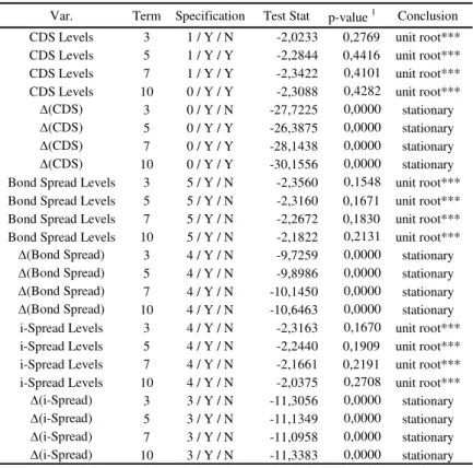
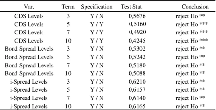
the existence of a unit root using ADF test10. To make sure the order of integration of the variables is I(1), first differences are also tested and, finally, confirmatory analysis is conducted on the variables in levels using KPSS11 test as above discussed. Table 4 summarises the results of ADF tests and, as one might anticipate, all series contained one unit root. Null hypothesis of a unit root could not be rejected for all variables in levels at 10% level, and was strongly rejected for all variables in first differences. KPSS test confirmed these results, as shown Table 5 for all variables in level.

Table 4 - Unit root testing

This table reports the results of ADF test conducted in CDS premium at 3, 5, 7 and 10 years maturities and the correspondent bond spreads and i-spreads. It included up to 1018 observations (sample adjusted from 20/03/2007 to 18/03/2011, depending on the number of lags selected) and the number of lags was selected according to Schwarz Info Criterion. Test regression included a constant for all variables and, because a trend could be identified in the data series under the null hypothesis, a trend for CDS premium at 5, 7 and 10 years, as indicated in specification column [Lags / Intercept (Y/N) / Trend (Y/N)]. * denotes null hypothesis cannot be rejected at 1% level, ** denotes null hypothesis cannot be rejected at

5% level, *** denotes null hypothesis cannot be rejected at 10% level. 1 denotes

MacKinnon, Haug et al. (1999) one-sided p-values.

Var. Term Specification Test Stat p-value 1 Conclusion CDS Levels 3 1 / Y / N -2,0233 0,2769 unit root*** CDS Levels 5 1 / Y / Y -2,2844 0,4416 unit root*** CDS Levels 7 1 / Y / Y -2,3422 0,4101 unit root*** CDS Levels 10 0 / Y / Y -2,3088 0,4282 unit root***

Δ(CDS) 3 0 / Y / N -27,7225 0,0000 stationary

Δ(CDS) 5 0 / Y / Y -26,3875 0,0000 stationary

Δ(CDS) 7 0 / Y / Y -28,1438 0,0000 stationary

Δ(CDS) 10 0 / Y / Y -30,1556 0,0000 stationary Bond Spread Levels 3 5 / Y / N -2,3560 0,1548 unit root*** Bond Spread Levels 5 5 / Y / N -2,3160 0,1671 unit root*** Bond Spread Levels 7 5 / Y / N -2,2672 0,1830 unit root*** Bond Spread Levels 10 5 / Y / N -2,1822 0,2131 unit root***

Δ(Bond Spread) 3 4 / Y / N -9,7259 0,0000 stationary

Δ(Bond Spread) 10 4 / Y / N -10,6463 0,0000 stationary i-Spread Levels 3 4 / Y / N -2,3163 0,1670 unit root*** i-Spread Levels 5 4 / Y / N -2,2440 0,1909 unit root*** i-Spread Levels 7 4 / Y / N -2,1661 0,2191 unit root*** i-Spread Levels 10 4 / Y / N -2,0375 0,2708 unit root***

Δ(i-Spread) 3 3 / Y / N -11,3056 0,0000 stationary

Δ(i-Spread) 10 3 / Y / N -11,3383 0,0000 stationary Augmented Dickey-Fuller Unit Root Test

10

H0: Series contains a unit root. Critical values for intercept / no trend: -3,4366 at 1% level; -2,8642 at

5% level and 2,5682 at 10% level. Critical values for intercept / linear trend: 3,9671 at 1% level; -3,4142 at 5% level and -3,1292 at 10% level; Fuller (1976).

11

H0: The series is stationary. Asymptotic critical values for intercept / no trend: 0,739 at 1% level; 0,463

(24)

Table 5 - Stationarity testing

This table reports the results of KPSS test for the same variables in levels. It included 1018 observations (sample from 20/03/2007 to 18/03/2011). Specification column indicates the inclusion of intercept and trend in the test [Intercept (Y/N) / Trend (Y/N)]. * denotes null hypothesis is rejected at 10% level, ** denotes null hypothesis is rejected at 5% level, *** denotes null hypothesis is rejected at 1% level.

Var. Term Specification Test Stat Conclusion

CDS Levels 3 Y / N 0,5676 reject Ho ** CDS Levels 5 Y / Y 0,5160 reject Ho *** CDS Levels 7 Y / Y 0,4920 reject Ho *** CDS Levels 10 Y / Y 0,4245 reject Ho *** Bond Spread Levels 3 Y / N 0,5302 reject Ho ** Bond Spread Levels 5 Y / N 0,5242 reject Ho ** Bond Spread Levels 7 Y / N 0,5180 reject Ho ** Bond Spread Levels 10 Y / N 0,5088 reject Ho ** i-Spread Levels 3 Y / N 0,6210 reject Ho ** i-Spread Levels 5 Y / N 0,6157 reject Ho ** i-Spread Levels 7 Y / N 0,6140 reject Ho ** i-Spread Levels 10 Y / N 0,6165 reject Ho **

KPSS Unit Root Test

Therefore, in order to avoid regressing non stationary series, a statistically valid model would be in first differences and, for this model to have a long run solution, a cointegrating relationship (suggested by the theory) should be found first and then it is valid to include this cointegrating term (which is also stationary), along with first differenced terms, in an error correction model in a second step.

Engle-Granger 2 step method

Step 1: Estimation of cointegrating equation

This method tests for cointegration in a regression using a residual based approach. For each maturity, the residuals of a standard OLS regression between the corporate yield spread and the CDS spread should be tested for the existence of a unit root. If this residual series can be considered stationary, one can conclude that the two variables are cointegrated. Therefore, the residuals (ut) of the following potential cointegrating

equation should be tested:

Bondspread t = γ 0 + γ 1 CDS t + ut (2)

If the residuals ut can be considered stationary, one can conclude for the existence of a cointegrating relationship between the two variables. In this case, the estimated

(25)

is know as the cointegrating term. In this case the cointegrating vector would be [1 -γˆ1].

The results for France Telecom are given in Table 6.

Table 6 - Estimated potentially cointegrating equations and residual tests for France Telecom

This table reports the results of standard OLS regression between corporate yield spreads and CDS prices and the correspondent residual tests using ADF and KPSS tests. The cointegrating equations are bondspreadt = γ 0 + γ 1CDSt + ut and i-spreadt = γ 0 + γ 1CDSt +

ut Included observations: 1018, from 20/03/2007 to 18/03/2011 for OLS regression and

KPSS test (and adjusted for ADF test depending of number of lags included). In ADF tests * denotes null hypothesis is rejected at 10% level, ** denotes null hypothesis is rejected at 5% level, *** denotes null hypothesis is rejected at 1% level. In KPSS tests * denotes null hypothesis cannot be rejected at 1% level, ** denotes null hypothesis cannot be rejected at 5% level, *** denotes null hypothesis cannot be rejected at 10% level.

Var. Term γ0 γ1 Test Stat. p-value 1 Conclusion Test Stat. Conclusion

Bond Spread 3 23,6597 1,3266 -3,4143 0,0107 Stationary ** 0,1151 Stationary *** Cointegrated Bond Spread 5 20,4752 1,2155 -2,6997 0,0744 Stationary * 0,2928 Stationary *** Cointegrated Bond Spread 7 23,0305 1,1563 -2,3801 0,1477 unit root*** 0,3891 Stationary ** Not Cointegrated Bond Spread 10 36,5349 0,9818 -2,0787 0,2535 unit root*** 0,4486 Stationary ** Not Cointegrated i-Spread 3 0,2585 1,0350 -3,2346 0,0184 Stationary ** 0,3639 Stationary ** Cointegrated i-Spread 5 7,0384 0,8936 -2,4160 0,1375 unit root*** 0,4639 Stationary * Not Cointegrated i-Spread 7 15,8963 0,8371 -2,0514 0,2649 unit root*** 0,5043 Stationary * Not Cointegrated i-Spread 10 37,6447 0,6746 -1,6841 0,4391 unit root*** 0,5507 Stationary * Not Cointegrated

esiduals KPSS Unit Root Te Residuals ADF Unit Root Test

Using the confirmatory data analysis, the conclusion from Table 6 is that bond spreads and CDS were cointegrated in the 3-year and 5-year maturity for France Telecom in the period in analysis. The cointegration between i-spreads and CDS only held for the 3-year term. The estimated slope coefficient in the cointegrating equation is close to unity, as expected from theory.

Step 2: Error correction model

The final step in this framework is to use a lag of the first step residuals, ût-1, in levels,

as the equilibrium correction term in the general equation when the cointegrating relation holds (the error correction model), or estimate a model with just differences if not. In the last case it will be a short term model. The overall model is:

Δ(bondspread)t = β 0 + β 1 Δ(bondspread)t-1 + α 1Δ(CDS)t-1 +δ ut-1 + εt (3)

(26)

number of models and found that lagged changes in future prices can help to predict spot price changes.

Table 7 reports the coefficient estimates for this model in the case of France Telecom. It is valid to analyse the signals and the significance of the coefficient estimates because

all variables in the equation are stationary. Considering first the Δ(CDS)t-1, the estimate

for α 1 is positive and highly significant for the four analysed maturities. This indicates

that CDS do indeed lead corporate yield spreads (both bond and i-spreads as above defined), since lagged changes in CDS prices lead to a positive change in the subsequent corporate yield spread.

Table 7 - Estimated error correction model for France Telecom

This table reports the results of standard OLS regression between corporate yield spread changes and lagged CDS changes, including an error correction term when cointegration holds. The equations are Δ(bondspread)t = β 0 + β 1 Δ(bondspread)t-1 + α 1Δ(CDS)t-1 +δ ut-1

+ εt and Δ(i-spread)t = β 0 + β 1 Δ(i-spread)t-1 + α 1Δ(CDS)t-1 +δ ut-1 + εt.. Included

observations: 1016 after adjustments, from 22/03/2011 to 18/03/2011.

Var. Term β0 p-value β1 p-value α1 p-value δ p-value Adj R-Square

Δ(Bond Spread) 3 0,0387 0,7369 -0,0959 0,0029 0,1886 0,0000 -0,0045 0,4131 0,0197

Δ(Bond Spread) 5 0,0363 0,7462 -0,0868 0,0060 0,1668 0,0001 -0,0099 0,0208 0,0242

Δ(i-Spread) 3 0,0135 0,8809 0,1505 0,0000 0,1175 0,0007 -0,0114 0,0078 0,0396

Δ(i-Spread) 5 0,0150 0,8618 0,1706 0,0000 0,1182 0,0002 - - 0,0408

β1 is the coefficient on lagged corporate yield spread. It is also highly significant,

indicating autocorrelation in corporate spreads (positive auto correlation in the case of

credit spread at 3 year maturity). Finally, δ, the coefficient on the error correction term, is negative and significant for bond spread at 5 year maturity and i-spread at 3 year maturity. This means that if the difference between corporate yield spreads and CDS is positive in one period, the corporate yield spreads will fall in the next to restore equilibrium, and vice versa. This dynamic could not be proved for the bond spread at 3

year maturity, as δ revealed not significant.

3.3 The Determinants of Basis Spread Changes

(27)

proxies of explanatory variables, namely Collin-Dufresne, Goldstein et al. (2001), Blanco, Brennan et al. (2005), Ericsson and Renault (2006), among others.

Longstaff, Mithal et al. (2005), in line with Elton, Gruber et al. (2001), argue that asymmetry in taxation between corporate bonds and treasuries may explain a portion of the basis, as treasures are exempted from local and state taxes and corporate bonds are not. Therefore, being CDS purely contractual in nature, CDS premium should not include a tax related component and reflect only the credit risk of the underlying entities. Another possible determinant of non default component appointed by Longstaff, Mithal et al. (2005) is the illiquidity of corporate bonds. Therefore these authors test for tax effects, using coupon rate as proxy and liquidity factors using the following proxies: average bid-ask spread, notional amount (to measure the overall availability), age, time to maturity of selected bonds, among others. They also perform a time series analysis against market liquidity measures. They report to have found evidence that the non default component is strongly related to liquidity measures, while for the taxation issues the results were not conclusive.

Zhu (2006) uses panel data techniques to explain the determinants of basis spread movements, and explanatory variables included lagged basis spreads, changes in CDS spreads, ratings and rating events, contractual arrangements (using dummy variables) liquidity factors (using bid-ask spreads in CDS and bond markets) and proxies for broad market conditions (including equity indexes).

The approach followed by Blanco, Brennan et al. (2005) in this respect has its roots in the work of Collin-Dufresne, Goldstein et al. (2001). They argue that yield spreads on corporate bonds occur for mainly two reasons: the possibility of default and the recovery rate (as the bond holder receives only a portion of the contracted payments, should the default occur). As such, they consider several variables as proxies for default component (namely changes in the spot interest rate, changes in the slope of the yield curve, changes in equity prices, changes in implied volatility) and for recovery rate (which they relate with overall business conditions). Additionally, they also refer to changes in liquidity affecting both changes in corporate spreads and CDS prices (and proxy it with on-the-run/off-the-run spread of long-dated US treasury yields). They use OLS regression individually for each reference entity and cross sectional regressions and pooled estimates.

(28)

liquidity, associated with general market characteristics, which include measures like conventional bid-ask spread, percentage quoted spread and other spread measures; and endogenous liquidity, connected with specific positions and exposure of one participant due to its own actions. In this respect, a study by Gaspar and Sousa (2010) provides an application of Bangia, Diebold et al. (1998) model to the insurance sector in Portugal, computing the liquidity risk using the percentage quoted spread.

Specific approaches to liquidity in corporate yield spreads include the works of Ericsson and Renault (2006) and Chen, Lesmond et al. (2007), as above discussed. They refer to different proxies for liquidity including bid-ask spreads of corporate bonds.

The above authors mainly focus on the effects of liquidity in bond markets, except for Zhu (2006), which specifically used CDS bid-ask spreads in his analysis. In this respect, another set of recent researches explore in more detail the effects of liquidity in CDS pricing, for example Yan and Tang (2007), that estimated a 20% liquidity premium in CDS prices, Bühler and Trapp (2009) and Fontana (2010), that explored the issue of counterparty risk in CDS markets and included as proxy the Libor-OIS spread (LOIS), arguing that if Libor 3 months is the rate which banks are willing to lend to each other and OIS the overnight rate on a derivative contract generally fixed by central bank and considered risk free in the US, the (widening of) gap between can be considered a measure of risk in the inter-bank lending market, because it reflects what the banks believes is the risk of default in lending to other banks.

Based upon the literature, it is now proposed the following variables to analyse the determinants of basis changes:

1. Lagged basis changes. With this variable it will be possible to evaluate the autocorrelation on the basis changes, specifically, and as stressed in Zhu (2006), being average basis a mean reverting process, a coefficient between 0 and 1 confirms the mean reverting feature (the smaller the faster the speed of adjustment to the long run equilibrium).

(29)

Figure 6 - Euribor-EONIA spread evolution in 2007-2011 period

0,0 1,0 2,0 3,0 4,0 5,0 6,0

02-01-07 02-07-07 02-01-08 02-07-08 02-01-09 02-07-09 02-01-10 02-07-10 02-01-11

Pe

rc

e

n

ta

g

e

Euribor 3M EONIA (EUSWEC)

(30)

Figure 7 - Bid-Ask spreads for France Telecom CDS (on top) and bond yields (bellow) 0 2 4 6 8 10 12 14 16 18 20

20-03-07 20-09-07 20-03-08 20-09-08 20-03-09 20-09-09 20-03-10 20-09-10 20-03-11

B a si s P o in ts 3Y 5Y 7Y 10Y 0 2 4 6 8 10 12 14 16 18

20-03-07 20-09-07 20-03-08 20-09-08 20-03-09 20-09-09 20-03-10 20-09-10

Ba s is P o in ts 3Y 5Y 7Y 10Y

4. Market conditions. In order to assess the effects of general market conditions, three variables are included: a volatility index, which tend to be associated with instability in the markets and with the risk of default (VDAX), an equity index (CAC 40 in this case) and one proxy for the country risk of default (France sovereign CDS at 5 year maturity in this case). After ensuring that all variables are I(1), the following model is applied:

(31)

Where EES denotes Euribor 3 months - EONIA spread and εt is an error term. Table 8

present the results for France Telecom.

Table 8 - Regression of basis spreads on counterparty and funding risks, liquidity and broad market conditions proxies for France Telecom

This table reports the results form regressing the CDS-Bond basis and CDS-i-Spread changes, in basis points, for maturities ranging from 3 years to 10 years, against the proxies of counterparty and funding risks, liquidity and broad market conditions. Included observations: 916 after adjustments, from 22/03/2007 to 18/03/2011.

Δ(CDS-Bond_Basis)t = β1Δ(CDS-Bond_Basis)t-1 + β2Δ(EES)t + β3Δ(BASCDS)t +

+ β4Δ(BASBond)t + β5Δ(VDAX)t + β6Δlog(CAC40)t +

+ β7Δ(CDSFrance)t + εt

Var. Term β1 β2 β3 β4 β5 β6 β7 Adj R-Squared N Δ(CDS-Bond Basis) 3 -0,0509 -0,0928 -0,0888 -0,0578 -0,0964 -58,8411 0,1517 0,0654 916

(0,1265) (0,0521) (0,354) (0,7737) (0,2940) (0,0000) (0,0049)

Δ(CDS-Bond Basis) 5 -0,0085 -0,1628 0,0547 -0,1162 -0,0677 -72,4846 0,1561 0,0996 916 (0,7918) (0,0008) (0,6446) (0,6154) (0,4680) (0,0000) (0,0044)

Δ(CDS-Bond Basis) 7 -0,0109 -0,1774 0,0311 -0,0566 -0,0103 -66,0059 0,1815 0,0944 916 (0,7349) (0,0003) (0,7864) (0,8323) (0,9140) (0,0000) (0,0011)

Δ(CDS-Bond Basis) 10 0,0159 -0,2162 0,4235 -0,2392 0,0051 -67,7470 0,1741 0,1272 916 (0,6145) (0,0000) (0,0000) (0,4574) (0,9569) (0,0000) (0,0019)

Δ(CDS-i-Spread Basis) 3 0,0842 0,0222 0,0009 0,3289 -0,0475 -58,2748 0,0847 0,0926 916 (0,0090) (0,6148) (0,9923) (0,0776) (0,5767) (0,0000) (0,0907)

Δ(CDS-i-Spread Basis) 5 0,1267 -0,0511 0,3975 0,3668 -0,0552 -69,4907 0,0890 0,1433 916 (0,0000) (0,2485) (0,0003) (0,0818) (0,5178) (0,0000) (0,0757)

Several findings emerge from Table 8. First, broad market conditions, except for the volatility index in this case, were highly significant in the period in analysis. The equity index had a negative impact on the basis across all maturities and its magnitude was stable. The perceived country risk of default had a positive impact on the basis but its magnitude was much greater in the CDS-Bond basis than in CDS-i-Spread Basis. Some authors may argue that in equilibrium these factors should be equally priced in both CDS and bond markets and therefore these variables should not be significant. Nevertheless, considering the crisis period, these findings supports the idea that in this period credit conditions was not efficiently priced in the two markets (or at least equally).

(32)

spreads, especially when using government bonds as benchmark, is less sensitive to this risk. This result did not hold entirely for the CDS-i-Spread basis. One possible explanation is that i-spreads uses swap curve as benchmark and swaps, being OTC products, may be more sensitive to counterparty risk than government risk free instruments, as above mentioned.

(33)

Chapter 4 Full Data Set

Having illustrated the general approach with France Telecom, it is now time to extend the analysis to a sample of investment graded firms in the eurozone using an extensive set of data from Bloomberg. This dataset includes CDS mid, bid and ask quotations for 3, 5, 7 and 10 years contracts and a full set of corporate bonds to cover the procedure above described, for the time period from 20th of March 2007 to the 18th of March 2011. The starting point was the reference entities included in the i-Traxx Europe index, published by Markit. The i-Traxx Europe is a CDS index covering reference entities from Financial, Auto & Industrial, Consumers, Energy and TMT (Telecommunications, Media and Technology), with maturities ranging from 3 to 10 years and with composition reviewed every 6 months. Table 9 summarizes the included data.

Table 9 - Dataset summary

This table summarizes the reference entities included in this project. The data covers investment graded reference entities from France, Germany, Italy, Portugal and Spain, and maturities from 3 years to 10 years.

Sector Country

Ratings S&P

(Jun 2011) Maturities Bonds Obs.

Allianz SE Financials Germany AA 5Y 7 847

Bay Motoren Werke AG Autos & Industrials Germany A - 3Y 5Y 6 1.017

Bertelsmann AG TMT Germany BBB + 3Y 5Y 5 1.024

Carrefour Consumers France BBB + 5Y 7Y 6 1.024

Cie de St Gobain Autos & Industrials France BBB 3Y 5Y 6 1.022

Deutsche Telekom AG TMT Germany BBB + 3Y 5Y 7Y 6 1.017

E.ON AG Energy Germany A 5Y 7Y 7 1.024

EDP Energias de Portugal Energy Portugal BBB 3Y 5Y 7Y 6 1.017

EDF Electricite de France Energy France A + 5Y 7Y 10Y 8 1.013

ENEL SpA Energy Italy A - 5Y 7Y 10Y 7 1.001

France Telecom TMT France A - 3Y 5Y 7Y 10Y 8 1.018

Iberdrola SA Energy Spain A - 5Y 7Y 4 1.023

Portugal Telecom TMT Portugal BBB - 5Y 7Y 10Y 5 1.012

Repsol YPF SA Energy Spain BBB 5Y 4 1.022

Telecom Italia SpA TMT Italy BBB 5Y 7Y 6 1.019

Telefonica SA TMT Spain A - 5Y 5 1.004

Veolia Environnement Energy France BBB + 5Y 7Y 10Y 5 1.024

101 17.128

The averages of the main project variables are detailed in Table 10, grouped by period12, sector, country and rating for the 5 year term. CDS-Bond basis is reported to be negative, -21,8 bp, for the period in analysis, and the CDS-i-Spread basis positive, 6,49

12

(34)

bp, and in line with previous studies. Blanco, Brennan et al. (2005) reported the basis at 5 year maturity to be 6 bp between 02/01/2001 and 20/06/2002, Zhu (2006) reported 13,25 bp between 01/01/1999 to 31/12/2002 and De Wit (2006) 16 bp between 01/01/2004 to 30/12/2005.

Table 10 - Average spreads of main variables for 5 year maturity

I II III IV All

CDS 34,17 88,81 182,16 114,33 105,06

Bond Spread 60,08 111,56 233,54 125,72 126,86

i-Spread 26,38 62,27 175,49 93,75 87,89

CDS-Bond Basis -25,92 -22,75 -51,38 -11,38 -21,80

CDS-i-Spread Basis 3,57 19,35 -17,57 10,30 6,49

BAS CDS 3,33 5,92 11,19 6,45 6,47

BAS Bond Yields 5,84 8,61 9,64 8,23 8,05

N 3.185 2.849 2.495 8.599 17.128

Autos & Ind. Consumers Energy Financials TMT All

CDS 135,17 60,79 99,08 79,05 113,03 105,06

Bond Spread 144,55 86,87 108,55 86,00 154,75 126,86

i-Spread 37,30 55,96 79,47 58,22 124,15 87,89

CDS-Bond Basis -9,38 -26,08 -9,47 -6,96 -41,72 -21,80

CDS-i-Spread Basis 8,18 4,83 19,61 20,83 -11,13 6,49

BAS CDS 7,98 5,56 6,65 6,76 5,89 6,47

BAS Bond Yields 7,93 8,60 8,01 8,37 8,01 8,05

N 2.039 1.024 7.124 847 6.094 17.128

France Germany Italy Portugal Spain All

CDS 84,03 93,26 159,67 120,06 113,15 105,06

Bond Spread 109,86 111,80 143,93 170,71 139,18 126,86

i-Spread 44,31 87,21 112,80 139,91 110,77 87,89

CDS-Bond Basis -25,83 -18,54 15,74 -50,65 -26,02 -21,80

CDS-i-Spread Basis 3,87 6,05 46,87 -19,85 2,38 6,49

BAS CDS 6,00 5,84 8,15 6,55 7,14 6,47

BAS Bond Yields 8,37 7,78 5,68 9,98 8,27 8,05

N 5.101 4.929 2.020 2.029 3.049 17.128

AA A + A A - BBB + BBB BBB - All

CDS 79,05 56,56 59,79 106,11 88,80 143,77 125,55 105,06 Bond Spread 86,00 63,06 80,04 110,03 122,09 168,12 209,50 126,86 i-Spread 58,22 37,80 49,93 84,72 92,11 93,35 178,09 87,89 CDS-Bond Basis -6,96 -6,50 -20,25 -3,92 -33,29 -24,34 -83,95 -21,80 CDS-i-Spread Basis 20,83 18,76 9,86 21,40 -3,31 5,60 -52,54 6,49

BAS CDS 6,76 3,99 4,19 6,32 6,08 8,28 6,10 6,47

BAS Bond Yields 8,37 7,69 8,32 7,61 7,92 8,09 10,50 8,05

N 847 1.013 1.024 5.063 4.089 4.080 1.012 17.128

(35)

Chapter 5 Lead-Lag and Long Term Relationship between CDS and

Bond Markets

This section reports the results for the cointegration and lead lag relationship between CDS and bond markets for the reference entities in analysis. As expected, all series contained one unit root in the period in analysis, as reported in Table A.1 in Appendix.

Considering first cointegration analysis, Table 11 (top) reports cointegration in 7 out of 17 studied cases in the 5 year maturity. Results for the full data set are presented in Appendix, Table A.3. Cointegration held in 33 out of 78, 42% of the analysed cases. Previous papers reported cointegration in more than 60% of the cases. In this respect, Blanco, Brennan et al. (2005) reported cointegration in 70% of the cases, between 02/01/2001 and 20/06/2002, Zhu (2006) reported 62,5%, between 01/01/1999 to 31/12/2002 and De Wit (2006) 61% between 01/01/2004 to 30/12/200513. This lower than expected result may be associated with the fact that the general market conditions are still not fully stabilized, with increasing prospects of an European sovereign debt crisis (March 2011).

The results for the error correction model regression are also presented in Table 11 (bottom) for bond spread in the 5 year maturity, and support the conclusion that CDS

spreads leads corporate yield spreads. The estimate for α 1 is positive and highly

significant in the great majority of the cases. This is in line with previous studies as Blanco, Brennan et al. (2005) and Zhu (2006) both report that CDS tends to lead bond markets.

13

(36)

Table 11 - Cointegration analysis and Lead-Lag relationship between CDS and bond markets for the reference entities in analysis

Reference Entity Var. Term α β Test Statistic p-value Conclusion Test Statistic Conclusion

Allianz SE Bond Spread 5 86,6373 -0,0080 -2,0182 0,2790 unit root*** 0,8814 reject Ho *** Not Cointegrated Bay Motoren Werke AG Bond Spread 5 16,1566 0,784207 -3,7883 0,0031 Stationary *** 0,2505 Stationary *** Cointegrated Bertelsmann AG Bond Spread 5 47,2746 0,9109 -2,8116 0,0569 Stationary * 0,7426 reject Ho *** Not Cointegrated Carrefour Bond Spread 5 11,5578 1,2389 -2,8050 0,0579 Stationary * 1,4230 reject Ho *** Not Cointegrated Cie de St Gobain Bond Spread 5 23,2276 1,0310 -5,1188 0,0000 Stationary 0,1034 Stationary Cointegrated Deutsche Telekom AG Bond Spread 5 9,9157 1,3252 -4,1994 0,0007 Stationary *** 0,1916 Stationary *** Cointegrated E.ON AG Bond Spread 5 15,1883 1,0846 -3,4684 0,0091 Stationary*** 1,1616 reject Ho *** Not Cointegrated EDP Energias de Portugal SA Bond Spread 5 56,7671 0,6575 -2,3775 0,1484 unit root*** 0,5978 Stationary * Not Cointegrated EDF Electricite de France Bond Spread 5 18,1239 0,7945 -3,4711 0,0090 Stationary *** 0,4547 Stationary ** Cointegrated ENEL SpA Bond Spread 5 47,8133 0,2547 -3,8102 0,0164 Stationary ** 0,1036 Stationary *** Cointegrated France Telecom Bond Spread 5 20,4752 1,2155 -2,6997 0,0744 Stationary * 0,2928 Stationary *** Cointegrated Iberdrola SA Bond Spread 5 20,9800 0,9631 -3,3142 0,0145 Stationary** 1,1017 reject Ho *** Not Cointegrated Portugal Telecom Bond Spread 5 71,0309 1,1029 -1,5430 0,5114 unit root*** 0,7422 reject Ho *** Not Cointegrated Repsol YPF SA Bond Spread 5 51,0528 0,8123 -3,9675 0,0017 Stationary*** 0,3553 Stationary ** Cointegrated Telecom Italia SpA Bond Spread 5 16,1828 1,0627 -3,5118 0,0386 Stationary ** 0,4141 reject Ho *** Not Cointegrated Telefonica SA Bond Spread 5 26,2484 1,0792 -3,2655 0,0168 Stationary** 1,1308 reject Ho *** Not Cointegrated Veolia Environnement Bond Spread 5 2,9048 1,3616 -2,5941 0,0945 Stationary * 1,4428 reject Ho *** Not Cointegrated

Residuals KPSS Unit Root Test Residuals ADF Unit Root Test

Reference Entity Var. Term β0 p-value β1 p-value α1 p-value δ1 p-value Adj R-Square

Allianz SE Δ(Bond Spread) 5 0,1134 0,4325 -0,3378 0,0000 0,0126 0,6795 - - 0,1118

Bay Motoren Werke AG Δ(Bond Spread) 5 0,0472 0,8287 -0,0067 0,8404 0,1223 0,0000 0,0039 0,5641 0,0172

Carrefour Δ(Bond Spread) 5 0,0605 0,6708 -0,1651 0,0000 0,2126 0,0001 - - 0,0360

Cie de St Gobain Δ(Bond Spread) 5 0,0584 0,6785 0,0022 0,9453 0,1476 0,0000 -0,0115 0,0160 0,0718

Deutsche Telekom AG Δ(Bond Spread) 5 0,0699 0,5950 -0,2107 0,0000 0,1726 0,0000 -0,0133 0,0248 0,0609

E.ON AG Δ(Bond Spread) 5 0,0416 0,7044 -0,0908 0,0037 0,1709 0,0000 - - 0,0217

EDP Energias de Portugal SA Δ(Bond Spread) 5 0,2064 0,1722 -0,1896 0,0000 0,1669 0,0000 - - 0,0560

EDF Electricite de France Δ(Bond Spread) 5 0,0773 0,5091 -0,2589 0,0000 0,0280 0,4771 -0,0423 0,0000 0,0942

ENEL SpA Δ(Bond Spread) 5 0,1106 0,4561 -0,3432 0,0000 0,1127 0,0000 -0,0160 0,0222 0,1507

France Telecom Δ(Bond Spread) 5 0,0363 0,7462 -0,0868 0,0060 0,1668 0,0001 -0,0099 0,0208 0,0242

Iberdrola SA Δ(Bond Spread) 5 0,1160 0,4545 -0,1072 0,0006 0,1512 0,0000 - - 0,0347

Portugal Telecom Δ(Bond Spread) 5 0,1502 0,5015 -0,0652 0,0510 0,2291 0,0000 - - 0,0389

Repsol YPF SA Δ(Bond Spread) 5 0,0686 0,6673 0,1296 0,0000 0,1957 0,0000 -0,0034 0,5250 0,1246

Telecom Italia SpA Δ(Bond Spread) 5 0,1086 0,6139 -0,1653 0,0000 0,2681 0,0000 - - 0,0912

Telefonica SA Δ(Bond Spread) 5 0,0813 0,5666 0,0081 0,7979 0,2453 0,0000 - - 0,0733

(37)

Chapter 6 The Determinants of the Basis Spread changes

This section reports the results from regressing the basis spread changes on proxies of counterparty and funding risks, liquidity in both CDS and bond markets and general market conditions. Figure 8 plots the time series of the variables in hand for reference entities in the energy sector. It documents an enormous increase of CDS prices for ENEL and Repsol during the 2008 crises, much greater than the increase observed for the other entities in the sector, with direct impact on the basis that was strongly positive in the first case.

Figure 8 – Regressing variables for energy sector

0 100 200 300 400 500 600 700

20-03-2007 20-09-2007 20-03-2008 20-09-2008 20-03-2009 20-09-2009 20-03-2010 20-09-2010

C D S Pr ice s ( B a s is Po in ts ) EON_CDS_5Y EDP_CDS_5Y EDF_CDS_5Y ENEL_CDS_5Y IBDR_CDS_5Y REP_CDS_5Y VEO_CDS_5Y -300 -200 -100 0 100 200 300 400 500 600

20-03-2007 20-09-2007 20-03-2008 20-09-200820-03-2009 20-09-200920-03-2010 20-09-2010

C D S-B o n d Basis ( B asis Po int s) EON_CDS-BOND_BASIS_5Y EDP_CDS-BOND_BASIS_5Y EDF_CDS-BOND_BASIS_5Y ENEL_CDS-BOND_BASIS_5Y IBDR_CDS-BOND_BASIS_5Y REP_CDS-BOND_BASIS_5Y VEO_CDS-BOND_BASIS_5Y 0 10.000 20.000 30.000 40.000 50.000

20-03-2007 19-10-2007 27-05-2008 23-12-2008 29-07-2009 26-02-2010 28-09-2010

0 4.000 8.000 12.000 16.000 FTSE_MIB DAX CAC_40 PSI_20 0 100 200 300 400 500 600

20-03-2007 20-09-2007 20-03-2008 20-09-200820-03-2009 20-09-2009 20-03-2010 20-09-2010

So v e re ig n C D S Sp re a d s (B a s is Po in ts ) GERMAN_CDS_SR_5Y PORTUGAL_CDS_SR_5Y FRANCE_CDS_SR_5Y ITALY_CDS_SR_5Y SPAIN_CDS_SR_5Y

Figure 8 also documents, from 2010, an increase of CDS spreads for Portuguese, Spanish and Italian local energy companies, probably related with the increasing country sovereign CDS spreads also above illustrated.

(38)

Counterparty and funding risks, proxied by the Euribor – EONIA spread, was significant in nearly 50% of the cases, mostly with the expected signal (negative), as much as the liquidity proxies, mostly in bond markets. Table A.5 in annex presents the results for CDS-i-Spread basis. Counterparty and funding risks revealed significant in approximately 40% of the cases, and liquidity in CDS markets in 65% of the cases.

Table 12 – Regression of CDS-Bond basis on counterparty and funding risks, liquidity and broad market conditions proxies

This table reports the results form regressing the CDS-Bond basis, in basis points, for 5 year maturity, on proxies of counterparty and funding risks, liquidity and broad market conditions. Included observations from 20/03/2007 to 18/03/2011.

Δ(CDS-Bond_Basis)t = β1Δ(CDS-Bond_Basis)t-1 + β2Δ(EES)t + β3Δ(BASCDS)t +

+ β4Δ(BASBond)t + β5Δ(VDAX)t + β6Δlog(Equity_Index)t +

+ β7Δ(CDSSovereign)t + εt

Reference Entity Var. Term β1 β2 β3 β4 β5 β6 β7

Adjusted R-squared _N

Allianz SE Δ(CDS-Bond Basis) 5 -0,0891 0,0720 0,1230 0,5019 0,1665 -89,0362 0,3909 0,1246 732 (0,0114) (0,3642) (0,4429) (0,0804) (0,2415) (0,0000) (0,0006)

Bay Motoren Werke AG Δ(CDS-Bond Basis) 5 0,0481 -0,5800 -0,2284 -1,2744 -0,2788 -216,3896 0,1572 0,1408 898 (0,1241) (0,0000) (0,0329) (0,0341) (0,1507) (0,0000) (0,3015)

Bertelsmann AG Δ(CDS-Bond Basis) 5 0,0329 -0,1550 0,2867 -0,5585 -0,1845 -107,4141 0,5842 0,0889 901 (0,3134) (0,0703) (0,0090) (0,2046) (0,2466) (0,0000) (0,0000)

Carrefour Δ(CDS-Bond Basis) 5 -0,0288 0,1121 -0,0026 -0,8511 0,4183 -42,9348 0,2872 0,1454 936 (0,3471) (0,0364) (0,9836) (0,0354) (0,0001) (0,0001) (0,0000)

Cie de St Gobain Δ(CDS-Bond Basis) 5 0,1403 0,0997 0,1438 0,4648 0,0042 -144,2223 0,4903 0,1978 934 (0,0000) (0,2459) (0,0857) (0,0934) (0,9804) (0,0000) (0,0000)

Deutsche Telekom AG Δ(CDS-Bond Basis) 5 -0,0247 0,0008 0,0583 0,0887 0,2781 -80,1579 0,0796 0,1244 879 (0,4390) (0,9892) (0,6334) (0,7018) (0,0075) (0,0000) (0,3281)

E.ON AG Δ(CDS-Bond Basis) 5 -0,0495 -0,0211 0,0248 -0,3998 0,0228 -70,0219 0,2257 0,1064 901 (0,1273) (0,6682) (0,8698) (0,0147) (0,8043) (0,0000) (0,0017)

EDP Energias de Portugal Δ(CDS-Bond Basis) 5 -0,0403 -0,1063 0,1289 -0,1336 0,4672 -62,4074 0,3022 0,3139 975 (0,1387) (0,1126) (0,1465) (0,5507) (0,0001) (0,0001) (0,0000)

EDF Electricite de France Δ(CDS-Bond Basis) 5 -0,1404 0,0177 0,2684 -0,5809 -0,2220 -90,3850 0,3514 0,1872 928 (0,0000) (0,7328) (0,0789) (0,0103) (0,0356) (0,0000) (0,0000)

ENEL SpA Δ(CDS-Bond Basis) 5 0,1436 -0,3209 0,5995 0,1866 0,6410 -75,3015 0,4943 0,2475 927 (0,0000) (0,0048) (0,0000) (0,6725) (0,0034) (0,0012) (0,0000)

France Telecom Δ(CDS-Bond Basis) 5 -0,0085 -0,1628 0,0547 -0,1162 -0,0677 -72,4846 0,1561 0,0996 916 (0,7918) (0,0008) (0,6446) (0,6154) (0,4680) (0,0000) (0,0044)

Iberdrola SA Δ(CDS-Bond Basis) 5 -0,0254 -0,2514 0,3216 -0,0567 0,3589 -80,6052 0,3435 0,2630 979 (0,3627) (0,0005) (0,0055) (0,8012) (0,0085) (0,0000) (0,0000)

Portugal Telecom Δ(CDS-Bond Basis) 5 -0,0256 0,2011 -0,0666 -0,5313 0,3162 -92,5720 0,1425 0,1314 970 (0,4080) (0,0199) (0,5897) (0,0055) (0,0387) (0,0000) (0,0000)

Repsol YPF SA Δ(CDS-Bond Basis) 5 0,0277 -0,1344 0,4869 0,1131 0,3364 -95,4194 0,2468 0,1665 978 (0,3484) (0,1482) (0,0000) (0,5901) (0,0598) (0,0000) (0,0000)

Telecom Italia SpA Δ(CDS-Bond Basis) 5 -0,0649 0,1483 -0,1139 -0,0956 0,8182 -83,6172 0,2773 0,1719 942 (0,0305) (0,1350) (0,1675) (0,8587) (0,0000) (0,0000) (0,0000)

Telefonica SA Δ(CDS-Bond Basis) 5 -0,0230 -0,0605 -0,0739 0,5193 -0,1303 -131,3340 0,1760 0,2426 964 (0,4173) (0,3191) (0,4491) (0,0056) (0,2922) (0,0000) (0,0000)

(39)

Chapter 7 Conclusions and Future Research

This project has examined the basis between CDS and corporate yield spreads and how CDS relates with those spreads. Even though significant deviations between the two measures are documented, especially during the crisis period, the analysis confirms the theoretical equilibrium predicted by theory. CDS and corporate bond yields should be on average equal. The error correction analysis performed suggests that cointegration between the two markets broadly holds and indicates that CDS prices do indeed lead corporate yield spreads.

During the analysis period, market conditions significantly affected the basis, as reported in the final regression analysis, both for CDS-Bond basis and for CDS-i-Spread basis, which are reported to be, on average, negative (-21,8 bp) in the first case and close to zero (6,49 bp) in the second between March 2007 and March 2011.

There is evidence that counterparty and funding risks significantly affected the basis, with negative impact in CDS prices and then in the basis, (particularly in the CDS-Bond basis). Liquidity proxies were found to be significant in more than 50% of the cases in the changes of bond basis spreads.

This project mainly focused in the effects of counterparty and liquidity risks in the basis and used Engle-Granger 2-step method to analyse cointegration and lead-lad relationship between CDS and bond markets. One of the problems in assessing cointegration in this framework is the lack of power in unit root testing and the impossibility to perform any hypothesis tests on the cointegrating relationship estimated in step 1. One step further would be to use more advanced techniques in this respect, namely the Johansen method to study cointegration and Vector Error Correction Model

and Granger Causality to study lead-lag relationship between CDS and bond markets.