Master in Applied Econometrics and Forecasting

(1)

Lisbon School of Economics & Management

Master in Applied Econometrics and

Forecasting

2016/2017

ESTIMATING GENDER DIFFERENCES IN THE PROBABILITY OF

UNEMPLOYMENT: EVIDENCE FROM PORTUGAL

Author:

Advisor:

(2)

ABSTRACT

By Joana M. Passinhas

Using a dynamic random effects probit model we estimate the probability of unemployment in Portugal in order to assess gender differences in average partial effects and in unemployment persistence, with data from four waves of the Survey on Income and Living Conditions (ICOR), for the period between 2010 and 2013. The estimation occurs while controlling for unobserved individual heterogeneity and for the

“initial conditions” problem, which arises from not knowing the stochastic process which originated the observed state of unemployment. We find strong evidence of persistence in unemployment, with some, although weak, evidence that men suffer more from the negative implications of previous unemployment. Simultaneously, we found evidence of higher probabilities of unemployment for women through a fixed effect that aimed to capture gender discrimination in an unstable labor market. The main contributions of the present work lie in the study of the determinants of the probability of unemployment, which represents a shortage in the current literature in labor economics, during a period of high unemployment in Portugal, and by having a special focus on unemployment persistence and gender discrimination.

JEL classification: C23, C25, J21, J24, J71

(3)

RESUMO

Por: Joana M. Passinhas

Através de um modelo dinâmico probit de efeitos aleatórios, estimou-se a probabilidade de desemprego em Portugal de forma a avaliar se existem diferenças entre géneros nos efeitos parciais médios e na persistência do desemprego. Os dados utilizados provêm do Inquérito ao Rendimento e Condições de Vida (ICOR) para o período entre 2010 e 2013. A estimação é feita ao mesmo tempo que se controla pela heterogeneidade individual não observada e pelo problema das condições iniciais, que ocorre pelo fato de não se conhecer o processo estocástico que originou o estado de desemprego observado. Encontrámos forte evidência empírica de persistência do desemprego, e alguma evidência de que esta persistência é mais pronunciada para os homens. Através da inclusão de um efeito fixo especifico para as mulheres, que pretende captar o efeito da discriminação de género num período de instabilidade no mercado de trabalho, concluímos que existe evidência estatística de maior probabilidade de desemprego para as mulheres. Este trabalho tem como principais contributos o estudo dos determinantes da probabilidade de desemprego, que representa uma carência da literatura em economia do trabalho, no fato de o estudar num período de grande desemprego em Portugal, e no especial enfoque que dá à persistência do desemprego e à discriminação de género.

JEL classification: C23, C25, J21, J24, J71

(4)

ACKNOWLEGDMENTS

(5)

LIST OF TABLES

TABLE 1 – DISTRIBUTION OF EMPLOYMENT STATUS ...23

TABLE 2 – DISTRIBUTION OF LEVELS OF EDUCATION ...24

TABLE 3 – AVERAGE PARTIAL EFFECTS ...30

TABLE A1 – VARIABLE DEFINITIONS AND EXPECTED EFFECTS ...40

TABLE A2 – DESCRIPTIVE STATISTICS OF THE VARIABLES ...41

TABLE A3 – DESCRIPTIVE STATISTICS OF THE VARIABLES FOR WOMEN ..41

TABLE A4 – EMPLOYED POPULATION ACCORDING TO MAIN OCCUPATION (ISCO-08) IN THOUSANDS (%∆) ...42

TABLE A5 – TRANSITION PROBABILITIES (FROM UNEMPLOYMENT OR EMPLOYMENT TO UNEMPLOYMENT) ...42

TABLE A6 – PANEL DATA MODELS FOR THE PROBABILITY OF UNEMPLOYMENT ...43

(7)

1. INTRODUCTION

In 2009, Portugal was facing its biggest government budget deficit to date (9.4% of the Gross Domestic Product (GDP)), one of the highest in all Euro Zone, and the pressure from the European Commission to reduce it, as well as to reduce the public debt (130.4% of GDP), was unbearable. In September of 2010, the Portuguese government announced an austerity package, with measures that focused on public administration pay cuts and raising taxes. In the same year, the deficit went to be the highest in Portuguese history, with a soaring value of 11% of GDP, much higher than what the

Maastricht Treaty (MT) and the Stability Growth Pact (SGP) established (3% of GDP). The year of 2011 was marked by both financial and political instability. With the country near bankruptcy, following the rejection of the Stability and Growth Pact IV (SGPIV) and the consequent resignation of the Prime Minister, the opposition parties asked for financial help to the “Troika” of the European Commission (EC), the European Central Bank (ECB) and the International Monetary Fund (IMF). As part of the deal, the Portuguese government agreed in reducing the public deficit to 3% until 2013 through another package of austerity measures1.

Over the period of 2010-20132 the GDP growth rate was negative, despite the positive growth of 2010 (1.9%) that was greatly influenced by a temporary growth of the private consumption driven by expectation of higher taxes over goods that ultimately led to an anticipation of acquiring durable goods. The falling growth rate of GDP also seemed to affect other economic indicators, with the unemployment rate following an abrupt increasing trend, reaching 16.2% in 2013. As a sub product of the crisis, the differential

1_{See Pereira &Weeman (2015) for more on the impact of the Global Financial Crisis in Portugal.}

(8)

in unemployment rates between men and women actually fell, from - 2.1 percentage points (p.p.) in 2010 to - 0.4 p.p. in 2013. The same did not happen with the participation rate that seemed to be unaffected by the crisis, maintaining the difference between men and women in approximately between 8 to 9 p.p., in all four years. This is consistent with evidence found in Albanesi & Şahin (2013) where the unemployment rate increased more for men than for women during the recent recessions, resulting from gender differences in industry distribution, due to the impact of those recessions on the construction and financial sectors, where the majority of the workforce is male.

As it has been for some time in Portugal, this was also a period marked by a demographic crisis, with the population falling at a -1.3% rate per year mostly because of emigration, especially high quality at working age emigration, and with a continued upward trend of the elderly population.

In this background of socio-economic crisis, we will focus on studying differences in the probability of unemployment between genders over a period of declining employment in Portugal, while controlling for relevant exogenous variables and unobserved individual heterogeneity. The causal effect of previous unemployment on current unemployment or the “scaring” effect of unemployment as it is known, will also be studied, especially to see if there is a difference between genders.

Moreover, we will seek to answer whether there are relevant differences in the probability of being unemployed and in the persistence of unemployment between men and women given a set of characteristics, in a period of high unemployment.

(9)

even when the attachment of women to the labor market had simultaneously increased. They conclude that this could be explained by labor market institutions, the impact of human capital differences and from the general easiness of indulging in prejudice against women, consequence of the excess of labor supply. These results reinforce the need to study a possible effect of gender discrimination in the probability of unemployment, especially in this high unemployment period for Portugal.

Secondly, to investigate the causes of the rise in European unemployment, that were perceived as not driven by exogenous shifts on the supply side, Arulampalam et al. (2000) found evidence of a casual effect of an individual’s previous unemployment experience on his future labor market condition. Past unemployment may be interpreted by employers as a signal of lower expected productivity, which eventually turns unemployment into a recurring cycle, therefore justifying the special interest in studying the effects of previous unemployment experience in the probability of unemployment.

Consequently, we explore the determinants of unemployment, of discrimination in the labor market and of persistence in unemployment by estimating dynamic panel data models of unemployment that allow to control for the effects of unobserved individual heterogeneity, after controlling for observable characteristics as education level, experience, age and number of kids.

(10)

unemployment for women, relatively to men, in spite of women having stronger presence in the higher levels of education.

We were also able to find strong state dependence effects with respect to previous unemployment incidence, during this period of high unemployment in Portugal, and weak evidence that unemployment persistence has a higher effect on the probability of unemployment for men.

The remainder of this paper is set out as follows. Section 2 reviews some important past literature on unemployment, discrimination in the labor market and unemployment persistence, Section 3 presents the econometric model, Section 4 describes the data set and Section 5 presents our estimates and results. The final section concludes and provides suggestions for further research.

2. LITERATURE SURVEY

The present survey of the literature will be divided in two sub-sections. The first aims to familiarize the readers of the relevant literature on theoretical models of labor discrimination while the second focus on providing useful insight on the causal relationships between unemployment and the considered determinants of unemployment.

2.1.THEORETICAL MODELS OF LABOR MARKET DISCRIMINATION The topic of discrimination in labor markets has been given a lot of attention in the last couple of decades. This attention has created two different approaches on the subject, taste-based discrimination and statistical discrimination.

(11)

2.1.1.TASTE-BASED DISCRIMINATION

Becker (1971) defines that someone has a “taste for discrimination” if he or she acts

as if he or she was willing to give up on some of his income in order to avoid interacting or to be associated with a member of a certain group.

When employers have a particular distaste in hiring someone from a particular group, say women, the cost of hiring a person from this group can be determined as the sum between the cost in terms of her wage and a measure of the disutility of hiring her. The measure of disutility will be interpreted as a discrimination coefficient, hereinafter referred to as 𝑑_𝑐.

The equilibrium happens when wages adjust to 𝑤_𝑀 = 𝑤_𝑊+ 𝑑_𝑐 , with 𝑤_𝑊 and 𝑤_𝑀 being, respectively, the wage of a woman and of a man, so that the market absorbs all female and male workers. If 𝑑_𝑐 is left to differ across employers, 𝑑_𝑐𝑗 with (𝑗 =

1, … , 𝐽), and 𝑑_𝑐𝑗 ≠ 0, then some employers would only hire men, if 𝑤_𝑀− 𝑤_𝑊< 𝑑_𝑐𝑗1, and some would only hire women, if 𝑤_𝑀 − 𝑤_𝑊> 𝑑_𝑐𝑗2, where 𝑗₁ ≠ 𝑗₂. Facing a constraint of parity of wages, and assuming that ∀ 𝑗 ∈ {1, … , 𝐽}: 𝑑_𝑐𝑗 > 0, then no woman would be employed.

2.1.2. STATISTICAL DISCRIMINATION

In Arrow (1973), employers’ discrimination is also considered as a result of their

perception of reality, reflecting the way they “perceive”, in an unequal manner,

expected performance of men relatively to women. This asymmetric perspective of the employers is based solely on which group each individual belongs to, male or female, and will mirror their experience or the social consensus regarding women’s

(12)

true productivity, the fact that some employer views male workers as having a higher probability of being qualified for the job, will result in higher unemployment rates for women. This problem is intensified with the existence of law enforcements that demand parity of wages, not enabling women to lower their wage rate in order to undertake the costs induced by statistical discrimination.

Phelps (1972) is the first to develop a model meant to explain statistical discrimination. This contribution was useful for building the foundations and inspiring a large number of models on discrimination. Notwithstanding, it did not, as Aigner & Cain (1977) state, focused on explaining economic discrimination as it assumed differences in ability for each group of individuals. For that reason, we will focus on Aigner & Cain’s (1977) model for explaining statistical discrimination.

This type of discrimination happens simply because employers can’t observe actual

(13)

evidence for this particular result, with employers reserving some jobs for men and others especially for women.

The distinction between these two types of discrimination has particularly important policy implications. For taste-based discrimination, policies should work on raising the cost of engagement in discriminatory behavior while for statistical discrimination policies should focus on providing and improving tools for obtaining information on job candidates.

2.2. UNEMPLOYMENT DETERMINANTS

According to INE, the national statistical institute in Portugal, someone is unemployed if he or she has been searching for work over the past four weeks, is

available for work and, currently, doesn’t have work. This follows the International

Labour Organization (ILO) measure of unemployment, which is meant to include, not the individuals who actively do not want to be in the labor market, but those who want to work but are not able to find any.

From this definition two possible reasons for unemployment emerge. One stemming

from productivity problems, where the person’s expected productivity is low and, therefore, delivers a marginal product that is expected to be less than the current wage rate. And one situation where the employer would be willing to hire, but the worker is not willing to supply labor at the current wage rate. This implies that both expected and true productivity are important factors that weigh in on both decisions: the

employers’ decision of hiring or not and the workers’ decision to accept, or not, an offer.

(14)

candidates acquired skills, the training and education levels that they have, their relevant work experience, and non-human-capital factors such as gender, race, age, if they have children or not and the age of the children.

Moreover, this expected productivity can be very different from the true productivity. It can also be overshadowed by a disutility that the employer might have in hiring from one group of people (taste based discrimination), or by an unjustified perception based on their personal characteristics (statistical discrimination).

2.2.1. GENDER DIFFERENCES IN UNEMPLOYMENT

There are many possible explanations for an existing gender gap regarding unemployment rates. An economic approach suggests examining both sides of the labor market to better evaluate these reasons.

(15)

the impact that the recent recessions had on the construction and financial sectors, where the majority of the workforce is male. They also found that the unemployment gender gap was highly affected by the labor attachment of each gender, and that the recent convergence of unemployment rates was related to an increase in labor attachment of women while, simultaneously, the labor attachment of men declined.

Şahin et al. (2010) also found evidence of higher unemployment rates for men in the recession of 2007, resulting from men dominating the most affected industries but also from the fact that a higher percentage of men tried to rejoin the labor force but were unable to find a job, therefore, transitioning from inactive status to unemployment status.

On the supply side, human capital accumulation, previous employment status, the number of kids, as well as different personal characteristics may be behind the gender gap in unemployment rates. Azmat et al. (2006) focused on explaining the cross-country differences in the gender unemployment gap. One important conclusion that they arrived was that differences in human capital accumulation were one of the most important part in explaining the flows from employment to unemployment, and vice-versa.

2.2.2. PERSISTENCE IN UNEMPLOYMENT

(16)

Arulampalam (2001) also found that previous unemployment had a negative impact on wages when individuals re-entered the job market. These effects are usually justified by the fact that past unemployment experience might result in depreciation of human capital, therefore raising one’s probability of unemployment, and/or by the fact that past unemployment is seen by employers as a signal of low productivity. They also conclude that unemployment persistence during a demand contraction – during less job opportunities – may be longer because on one hand, perceived average quality of the unemployed is lower and, on the other hand, the poor economic conditions will result in fewer job vacancies being open, which will enhance the demand contraction. Some studies (e.g. Elmeskov & MacFarlan, 1993) have also stated that persistence of higher than usual unemployment could actually be a result of an increase of the natural rate of unemployment and therefore could actually never fully correct itself to the previous level. The same article also studies the “hysteresis” phenomenon as an alternative explanation to the persistence of unemployment where, according to this view, the structural unemployment rate depends fully, or partially,

on the current unemployment rate. The authors use the “scarring” effect of

unemployment as a source of the “hysteresis” phenomenon citing that long periods of unemployment lead to less training opportunities, to depreciation of human capital. Additionally, past unemployment may be interpreted by employers as a signal of lower expected productivity, which eventually turns unemployment into a recurring cycle.

(17)

2.2.3.UNEMPLOYMENT AND HUMAN CAPITAL EDUCATION

If we think of the theory of the firm, we recall that the simplest assumption is that firms try to maximize their profits. This assumption is then used to explain firms’ decisions regarding their economic activity, which also contemplates the decision regarding the amount of labor being used. From the employer’s perspective, hiring is an investment decision. They need to evaluate both the expected returns of labor, measured as expected productivity, as well as the risk of this expected productivity being less than the true productivity, while trying to maximize profits.

(18)

education gap and, in some countries, to even reverse it. Regardless, this similarity in educational levels was not followed by an equal choice of educational field, with women having greater presence in the areas of education, health and welfare, and humanities and arts while men still dominate engineering, manufacturing and construction, in OECD countries3. One important sub product of this asymmetry is gender segregation in occupation that has been suggested as the main cause in the existing gender pay gap.

These past years of some educational transformation suggest that the study of gender discrimination in the labor market should not continue to emphasize so much on the differences in education levels but instead relate it to other factors, for example, the impact of choosing male or female dominant fields of education.

EXPERIENCE

Employers, as most economic agents, make decisions based on limited information. Therefore, the greatest amount of available information allows for better predictions of expected productivity and for reducing the risk that arises when employing someone. Experience plays an important role in providing valuable information to the

employer by signaling, through the candidates’ previous work experience, if he or she

would be a good fit to both the company and the job. In fact, according to human capital theory, the skills accumulated through experience raise the probability of being employed in the future.

As gender differences in educational levels become less and less relevant, with both men and women attaining similar levels of schooling, differences in actual experience have narrowed less (possibly from the differences in chosen fields of study, women’s

(19)

seemingly preference for part time or temporary jobs and the fact that domestic work is still performed by women). As a result, their impact on unemployment incidence is especially important in developed countries that for have no gender gap in education. For example, according to Blau & Kahn (1997), women’s lower levels of human capital (especially lower levels of full-time experience) explain close to one third of the pay gap. Manning & Swaffield (2005) also found that, despite the approximately nonexistent pay gap, in the UK, when entering the labor market, there is a significant disparity past 10 years of entering it. They conclude that, although a large component of this difference is unexplained, human capital accounts for half of it, mainly thorough gender differences in on-the-job training and in accumulated experience.

2.2.4. UNEMPLOYMENT AND CHILDREN

Until now, we have focused our study on the impact that human-capital characteristics have on the probability of being unemployed. We have left an important part to take in consideration, which involves the aspects of raising kids, or having them, while searching for work. When studying the cross-country differences in the unemployment gender gap, Azmat et al. (2006) found that the gender gap in unemployment rates is larger for those who are married and those who have young children.

This might result from the fact that women can most likely be over-represented in part-time jobs (see Petrongolo (2004)). This job allocation is said to reflect women’s preferences specially their need to combine work with child care, although some cases this part time employment is involuntary.

(20)

1985, this association in OECD countries remains negative. This result can hinder future employment for women as they will have lower levels of experience than their male counter parts and may suffer more from the scarring effect of unemployment. The possibility that women at this age decide to have kids and voluntarily stay out of the labor force, but also from the general perception that a long maternity would lead to depreciation of the human capital stock and costs in temporary replacement, which eventually works as an obstacle for employment. These conclusions enhance the importance of estimating different impacts that family attributes have on the probability of a woman to be unemployed.

2.2.5. UNEMPLOYMENT AND OCCUPATIONAL SEGREGATION Preferences over future occupations become more complex and narrower as a person grows up. One of the first criteria for shorting the list of possible future occupations is

eliminating the ones that are perceived to be socially inappropriate for the person’s

sex (Gottfredson, 1981). This, combined with an image of who they would like to be, are some of the reasons that explain occupational segregation, as well as educational segregation.

Therefore, it is plausible to assume that the fact that society perceives some roles as strictly female or strictly male, have an extremely important impact creating gender differences both on the pursued fields of education, as well as the chosen economic occupation (see Cejka & Eagly (1999) or Wright et al. (2015)). This may, in itself,

create a “snowball” effect if it strengthens the gender-occupation stereotype, which would, most likely, result in more statistical discrimination.

(21)

is likely that some type of discrimination, either taste-based or statistical, might be contributing to the high employment rate of men. An analogous conclusion comes from female-dominant occupations. Consequently, differences in employment rates (and, therefore, unemployment rates) regarding gender must be correlated with prevailing gender segregation in economic occupations. In fact, some studies conclude that gender stereotypes might be preventing women from being hired and/or promoted in particular occupations, hindered by gender roles (e.g., Eagly & Karau, 2002).

Another matter that makes occupational gender segregation an important factor when studying gender discrimination is the fact that it is thought to be one of the main explanations for the gender gap in earnings of the current time, where women are as much educated as men (Gauchat et al. 2012). It is also perceived as economical inefficient as the lack of gender representation might keep talented individuals from occupying roles that they would be a great fit. This will result in lower overall productivity and economic growth that otherwise could come from unconstrained choices.

3. THE MODEL

The econometric specification is based on a binary dependent variable, 𝑦_𝑖𝑡, which takes on the value one if the individual 𝑖 is unemployed at time 𝑡 and zero otherwise.

Consider the following dynamic model assuming that 𝑦_𝑖0, the initial condition of 𝑦_𝑖𝑡, is the value for 𝑦 for each individual 𝑖 in 2010

𝑦𝑖𝑡 = 𝟏[ 𝒛𝒊𝒕𝜸𝟏+ 𝒛𝒊𝒕𝜸𝟐𝒅𝒇𝒊+ 𝜌1𝑦𝑖𝑡−1+ 𝜌2𝑦𝑖𝑡−1𝑑𝑖𝑓+ 𝜑𝑖 + 𝑣𝑖𝑡 ≥ 0] (1)

𝑖 = 1, … , 𝑛; 𝑡 = 1, … , 𝑇

(22)

explanatory variables (such as education, experience, number of kids and age), 𝑑_𝑖𝑓 is a dummy variable that equals one if the individual 𝑖 is a woman, 𝜸𝟏 is a 𝐾 × 1 vector of parameters associated with 𝐳_𝐢𝐭, 𝜸𝟐 is a 𝐾 × 1 vector of parameters associated with the interaction between 𝑑_𝑖𝑓and 𝐳_𝐢𝐭, 𝜌1 is the parameter that reflects the persistence of unemployment for men, 𝜌2 is the parameter that reflects differences between genders for the persistence of unemployment, 𝑣_𝑖𝑡 is the idiosyncratic error term and 𝜑_𝑖 is the unobserved heterogeneity term, constant in time.

In order to obtain 𝐷(𝑦_𝑖𝑡| 𝒛_𝒊𝒕, 𝑦_𝑖𝑡−1, 𝜑_𝑖), the following two assumptions are made Assumption 1:

𝐷(𝑦𝑖𝑡| 𝒛𝒊𝒕, 𝑦𝑖𝑡−1, 𝜑𝑖) = 𝐷(𝑦𝑖𝑡|𝑦𝑖𝑡−1, … , 𝑦𝑖0, 𝒛𝒊𝒕, 𝜑𝑖) (2)

Assumption 2: 𝑓_𝑡(𝑦_𝑡| 𝒛_𝒕, 𝑦_𝑡−1, 𝜑; 𝜽) is a correctly specified probability function for the conditional distribution on the left side of equation (2), where 𝜽 is a vector of parameters.

These two assumptions imply that the dynamics are correctly specified and that 𝒛_𝒊𝒕=

{ 𝒛𝒊𝟏, … , 𝒛𝒊𝑻} is strictly exogenous, conditional on 𝜑𝑖. Moreover, because it doesn’t

restrict the distribution of 𝜑_𝑖, it allows for dependence between the unobserved effects and 𝒛_𝒊𝒕.

Furthermore, these assumptions imply that the probability function of (𝑦_𝑖1, … , 𝑦_𝑖𝑇) given (𝑦_𝑖0 = 𝑦₀, 𝒛_𝒊𝒕 = 𝒛_𝒕, 𝜑_𝑖 = 𝜑) is ∏𝑇_𝑡=1𝑓_𝑡(𝑦_𝑡| 𝒛_𝒕, 𝑦_𝑡−1, 𝜑; 𝜃₀), with 𝜽_𝟎 equal to the true value of 𝜽. Therefore, this probability function depends on an unobservable term, 𝜑, and because of that, is not useful for inference. One solution to overcome this problem would be to consider 𝜑 as a fixed effect, resulting in the estimation of

(23)

problem4 when T is fixed, resulting in highly biased estimates of γ.

Wooldridge (2005) solves this problem by using the density of (𝑦_𝑖1, … , 𝑦_𝑖𝑇) conditional on (𝑦_𝑖0, 𝒛_𝒊). Because we already know the density of (𝑦_𝑖1, … , 𝑦_𝑖𝑇) conditional on

(𝑦𝑖0= 𝑦0, 𝒛𝒊𝒕 = 𝒛𝒕, 𝜑𝑖 = 𝜑), we only need to specify the density of 𝜑𝑖 conditional on

(𝑦𝑖0, 𝒛𝒊𝒕) and assume that it is correctly specified, which leads to Assumption 3.

Assumption 3: ℎ(𝜑|𝑦₀, 𝒛; 𝜶) is a correctly specified model for the density of

𝐷(𝜑𝑖|𝑦𝑖0, 𝒛𝒊) with respect to a 𝜎-finite measure 𝜂(𝑑𝜑), where 𝜶 is some vector of

parameters with the true value equal to 𝜶_𝟎.

Under assumptions 1,2 and 3, the density of (𝑦_𝑖1, … , 𝑦_𝑖𝑇) given (𝑦_𝑖0 = 𝑦₀, 𝒛_𝒊= 𝒛, 𝜑_𝑖 =

𝜑) is

∫ ∏_ℝ𝐽 𝑇𝑡=1𝑓𝑡(𝑦𝑡| 𝒛𝒕, 𝑦𝑡−1, 𝜑; 𝜽𝟎)ℎ(𝜑|𝑦0, 𝒛; 𝜶𝟎)𝜂(𝑑𝜑)

Leading to the following log-likelihood function for each observation

𝑙𝑖(𝜽, 𝜶) = log [ ∫ ∏ 𝑓𝑡(𝑦𝑡| 𝒛𝒕, 𝑦𝑡−1, 𝜑; 𝜽𝟎) 𝑇

𝑡=1

ℎ(𝜑|𝑦0, 𝒛; 𝜶𝟎) ℝ𝐽

𝜂(𝑑𝜑)] (3)

To estimate 𝜽_𝟎 and 𝜶_𝟎, Wooldridge (2005) uses the conditional Maximum Likelihood Estimator by summing the log-likelihood in equation (3) across 𝑖 = 1, … , 𝑁 and maximizing with respect to 𝛉 and 𝛼. This yields √𝑁-consistent and asymptotically normal estimators, under standard regularity conditions.

Let us now consider that the unobserved heterogeneity term (𝜑_𝑖) has a common part for both genders (𝜑_0𝑖) and a fixed effect for women (𝜃). Therefore, we can write 𝜑_𝑖 as

𝜑𝑖 = 𝜑0𝑖+ 𝜃𝑑𝑖𝑓.

Consequently, we can rewrite equation (1) as the following

(24)

𝑦𝑖𝑡 = 𝟏[ 𝒛𝒊𝒕𝜸𝟏+ 𝒛𝒊𝒕𝜸𝟐𝒅𝒊𝒇+ 𝜌1𝑦𝑖𝑡−1+ 𝜌2𝑦𝑖𝑡−1𝑑𝑖𝑓 + 𝜑0𝑖+ 𝜃𝑑𝑖𝑓 + 𝑣𝑖𝑡 ≥ 0] (4)

From the literature survey, we are aware that one of the reasons behind the gap in unemployment rates is taste-based discrimination and statistical discrimination. The latterhappens when the employer discriminates women, not because he or she has any disutility towards them, but because his/her general perception is that women have less ability than their male counterparts. Therefore, it is not restrictive to assume that women would have higher probabilities of unemployment in occupations where their perceived ability is lower, e.g. on activities that are usually thought to be reserved for men and, consequently, this fixed effect for women 𝜃, could also reflect that interesting result. In fact, because we aim to control for true individual ability, a difference between genders in the probability of unemployment should be associated with some type of discrimination which, has we have seen previously, usually leads to occupational segregation, that is said to be one of the causes behind the still existing wage gap. Then, this fixed effect aims to capture all types of discrimination that contribute to a possible gender gap in the probability of unemployment.

Finally, we are left to choose the density for the random unobserved heterogeneity term.

We will adopt Mundlak’s version of Chamberlain’s assumption as in Wooldridge (2010), with the addition of conditioning on 𝑦_𝑖0 as well.

To specify the density of 𝜑_0𝑖 conditional on (𝑦_𝑖0, 𝒛_𝒊), consider the following specification

𝜑0𝑖 = 𝛼0+ 𝛼1𝑦𝑖0+ 𝒛𝒊𝜶𝟐+ 𝑎𝑖 where 𝑎𝑖|𝑦𝑖0, 𝒛𝒊~𝑁(0, 𝜎𝑎2) (6)

and 𝒛_𝒊 is a vector that contains the average value, for each individual, for all covariates that vary over time.

(25)

𝜑0𝑖|𝑦𝑖0, 𝒛𝒊 ~ 𝑁(𝛼0+ 𝛼1𝑦𝑖0+ 𝒛𝒊𝜶𝟐, 𝜎𝑎2) (7)

In conclusion, 𝑦_𝑖𝑡 given (𝑦_𝑖𝑡−1, … , 𝑦_𝑖0, 𝒛_𝒊, 𝑎_𝑖, 𝑑_𝑖𝑓) follows a dynamic probit model with unobserved effects with the following specification

𝑃(𝑦𝑖𝑡 = 1|𝑦𝑖𝑡−1, … , 𝑦𝑖0, 𝒛𝒊𝒕, 𝜑𝑖𝑡, 𝑑𝑖𝑓) =Φ[ 𝒛𝒊𝒕𝜸𝟏+ 𝒛𝒊𝒕𝜸𝟐𝒅𝒊𝒇 + 𝜌1𝑦𝑖𝑡−1+ 𝜌2𝑦𝑖𝑡−1𝑑𝑖𝑓 +

𝜃𝑑_𝑖𝑓+ 𝛼1𝑦𝑖0+ 𝒛𝒊𝜶𝟐+ 𝑎𝑖] (8)

3.1.ESTIMATING AVERAGE PARTIAL EFFECTS

Our aim is to estimate the partial effect of each explanatory variable in equation (8). Because it is a nonlinear function, it will depend on the observed values of the variables, therefore, we will need to estimate the average partial effects (APEs). However, the APEs depend on unobserved variables (𝜑_𝑖), therefore Wooldridge (2005, 2010) suggests to average APEs across the distribution of 𝜑_𝑖. The expectation of model (8) gives,

𝜇(𝒛, 𝑦−1) = 𝐸 [Φ[𝒛 𝜸𝟏+ 𝒛 𝜸𝟐𝑑𝑖𝑓+ 𝜌1𝑦−1+ 𝜌2𝑦−1𝑑𝑖𝑓+ 𝜃𝑑𝑖𝑓+ 𝛼1𝑦𝑖0+ 𝒛𝒊𝜶𝟐

+ 𝑎𝑖]] (9)

where the expectation is with respect to the distribution of 𝑎_𝑖, 𝒛 and 𝑦₋₁ are possible values of𝒛_𝒕 and 𝑦_𝑡−1, respectively.

It is possible to obtain a consistent estimator of equation (9) using iterated expectations leading to,

𝐸{𝐸[Φ( 𝒛𝜸𝟏_{+ 𝒛 𝜸}𝟐_𝑑

𝑖𝑓+ 𝜌1𝑦−1+ 𝜌2𝑦−1𝑑𝑖𝑓+ 𝜃𝑑𝑖𝑓+ 𝛼1𝑦𝑖0+ 𝒛𝒊𝜶𝟐+ 𝑎𝑖|𝑦𝑖0,𝒛𝒊]} (10)

The conditional expectation inside equation (10) given (7) is

Φ(𝒛𝜸𝒂𝟏+ 𝒛𝜸𝒂𝟐𝑑𝑖𝑓+ 𝜌𝑎1𝑦−1+ 𝜌𝑎2𝑦−1𝑑𝑖𝑓+ 𝜃𝑎𝑑𝑖𝑓+ 𝛼𝑎1𝑦𝑖0+ 𝒛𝒊𝜶𝒂𝟐) (11)

where the ‘a’ subscript denotes the original parameter multiplied by (1 + 𝜎2

(26)

A consistent estimator of the expected value of (11) with respect to the distribution of (𝑦_𝑖0, 𝒛_𝒊) at time 𝑡 is

𝑁−1_∑_Φ_(𝒛

𝒊𝒕𝜸̂𝒂𝟏+ 𝒛𝒊𝒕𝜸̂𝒂𝟐𝑑𝑖𝑓+ 𝜌̂𝑎1𝑦𝑖𝑡−1+ 𝜌̂𝑎2𝑦𝑖𝑡−1𝑑𝑖𝑓+ 𝜃̂𝑎𝑑𝑖𝑓+ 𝛼̂𝑎1𝑦𝑖0+ 𝒛𝒊𝜶̂𝒂𝟐) 𝑁

𝑖=1

(12)

where the ‘a’ subscript now denotes multiplication by (1 + 𝜎̂2_𝑎)−1 2⁄ and the estimates of the parameters may be obtained with a random effects probit or a pooled probit, where the former estimates the “unscaled” parameters and 𝜎2_𝑎, while the pooled probit estimate directly the scaled parameters.

Therefore, the average partial effect of a generic dummy variable, say the k-th variable of the vector 𝒛_𝒊𝒕, will be, for a man and for a woman, respectively, equal to the following

𝐴𝑃𝐸

̂_𝑘𝑡 _{= 𝑁}−1_{∑ _[_Φ_(𝒛

𝒊𝒕𝒌−𝟏𝜸̂𝒂𝟏,𝒌−𝟏+ 𝛾̂𝑘𝑎1,𝑘−1+𝜌̂𝑎1𝑦𝑖𝑡−1+𝛼̂𝑎0+𝛼̂𝑎1𝑦𝑖0+ 𝒛̅𝜶̂𝒊 𝒂𝟐) − 𝑁

𝑖=1

Φ(𝒛𝒊𝒕𝒌−𝟏𝜸̂𝒂𝟏,𝒌−𝟏+𝜌̂𝑎1𝑦𝑖𝑡−1+𝛼̂𝑎0+𝛼̂𝑎1𝑦𝑖0+ 𝒛̅𝜶̂𝒊 𝒂𝟐)]} if 𝑖 is a man

𝐴𝑃𝐸

̂_𝑘𝑡 _{= 𝑁}−1_{∑ _[_Φ_(𝒛

𝒊𝒕𝒌−𝟏(𝜸̂𝒂𝟏,𝒌−𝟏+ 𝜸̂𝒂𝟐,𝒌−𝟏) + 𝛾̂𝑘𝑎1,𝑘−1+ 𝛾̂𝑘𝑎2,𝑘−1+(𝜌̂𝑎1+ 𝜌̂𝑎2)𝑦𝑖𝑡−1+ 𝑁

𝑖=1

𝜃̂𝑎 + 𝛼̂𝑎1𝑦𝑖0+ 𝒛𝒊𝜶̂𝒂𝟐) −

Φ(𝒛𝒌−𝟏(𝜸̂𝒂𝟏,𝒌−𝟏+ 𝜸̂𝒂𝟐,𝒌−𝟏)+(𝜌̂𝑎1+ 𝜌̂𝑎2)𝑦𝑖𝑡−1+ 𝜃̂𝑎+ 𝛼̂𝑎1𝑦𝑖0+

𝒛𝒊𝜶̂𝒂𝟐 )]}

if 𝑖 is a woman

where 𝒛𝒌−𝟏 is a 1 × (𝐾 − 1) vector containing the first 𝐾 − 1 variables of 𝒛 and 𝜸̂_𝒂𝒈,𝒌−𝟏 is the correspondent vector of parameters for 𝑔 = 1,2.

While for some variable 𝑧𝑗 (continuous) it will simply be,

𝐴𝑃𝐸

̂_𝑗𝑡 _{= 𝜸̂}_𝒂𝒋𝟏 1

𝑁∑𝑁𝑖=1𝜙(𝒛𝒊𝒕𝜸̂𝒂𝟏+𝜌̂𝑎1𝑦𝑖𝑡−1+𝛼̂𝑎0+𝛼̂𝑎1𝑦𝑖0+ 𝒛𝒊𝜶̂𝒂𝟐) if 𝑖 is a man

𝐴𝑃𝐸̂𝑗𝑡= (𝜸̂𝒂𝒋𝟏 + 𝜸̂𝒂𝒋𝟐)_𝑁1∑𝑁𝑖=1𝜙(𝒛𝒊𝒕𝜸̂𝒂𝟏+ 𝒛𝒊𝒕𝜸̂𝒂𝟐+𝜌̂𝑎1𝑦𝑖𝑡−1+ 𝜌̂𝑎2𝑦𝑖𝑡−1+ 𝜃̂𝑎+ 𝛼̂𝑎1𝑦𝑖0+

(27)

Then, APEs are √𝑁 consistent and asymptotically normal distributed. Their standard error can be obtained using the delta method or bootstrap.

3.2.ESTIMATING THE EFFECTS OF PREVIOUS UNEMPLOYMENT To study the effects of previous unemployment on current unemployment, we will estimate the probability of unemployment at time 𝑡 of the individual 𝑖 if he or she was unemployed at time 𝑡 − 1. This probability will be obtained for both genders and, subsequently, analyzed for the existence of significant dissimilarities between genders. This results in estimating the following probabilities for men and women, respectively

𝑃(𝑦𝑖𝑡 = 1|𝑦𝑖𝑡−1 = 1, 𝑑𝑓𝑖 = 0, … , 𝑦𝑖0, 𝒛𝒊𝒕) =Φ[ 𝒛𝒊𝒕𝜸𝟏+ 𝜌1+ 𝛼0+𝛼1𝑦𝑖0+ 𝒛̅𝜶𝒊 𝟐+ 𝑎𝑖]

𝑃(𝑦𝑖𝑡 = 1|𝑦𝑖𝑡−1 = 1, 𝑑𝑓𝑖 = 1, … , 𝑦𝑖0, 𝒛𝒊𝒕) =Φ( 𝒛𝒊𝒕𝜸𝟏+ 𝒛𝒊𝒕𝜸𝟐+ 𝜌1+ 𝜌2 + 𝜃 +

𝛼1𝑦𝑖0+ 𝒛𝒊𝜶𝟐+ 𝑎𝑖)

Another important estimate that enables the study of unemployment persistence, is the APE of the lagged dependent variable which consists in obtaining the following estimates for men and women, respectively

𝐴𝑃𝐸̂𝑈𝑁𝑡=_𝑁1∑ [𝑃(𝑦𝑁𝑖=1 𝑖𝑡 = 1| 𝒛𝒊𝒕, 𝑦𝑖𝑡−1= 1, 𝑑𝑓𝑖 = 0) − 𝑃(𝑦𝑖𝑡 = 1| 𝒛𝒊𝒕, 𝑦𝑖𝑡−1= 0, 𝑑𝑓𝑖 = 0)]

𝐴𝑃𝐸

̂_𝑈𝑁𝑡 ₌ 1

𝑁 ∑[𝑃(𝑦𝑖𝑡 = 1| 𝒛𝒊𝒕, 𝑦𝑖𝑡−1= 1, 𝑑𝑓𝑖 = 1) − 𝑁

𝑖=1

𝑃(𝑦𝑖𝑡 = 1| 𝒛𝒊𝒕, 𝑦𝑖𝑡−1= 0, 𝑑𝑓𝑖 = 1)]

4. THE DATA AND VARIABLES

(28)

final sample has been chosen so that all individuals remain in every wave. This is an important constraint as the econometric analysis we are going to perform requires a lag of unemployment in order to study its persistence. In addition, to ease the estimation of the initial conditions, it was chosen a common date of entry 2010 in order to assume that 𝑦_𝑖2010 is the initial condition of 𝑦 for each individual 𝑖. Furthermore, we removed individuals who had missing relevant information in any year and, since our aim is to study the active population (employed or unemployed status), the individuals who were not in the labor market for some year, at the time of the interview, were also dropped. The final sample resulted in 774 individuals observed in all 4 waves, from 2010 to 2013, with 384 women and 390 men.

The measure of unemployment used throughout this work is based on the ILO definition of unemployment, i.e., a person is considered unemployed if he or she does not have a job, has looked for work in the past four weeks and is available for work.

(29)

number of kids. As a limitation, it was not possible to identify the unemployment status of his or her spouse for 1,4% of the individuals who were married in the sample.

The raw unconditional probability of being unemployed for each wave is presented in Table 1. It also displays the distribution of employment status, over the four-year period.

This table shows evidence of higher female participation on part time employment, for all years. As mentioned in the literature review, some women tend to search and accept jobs that enables for temporary leave or less working hours, so that they can take care of

children, while men don’t generally search for the same conditions. It is also possible to notice that 2012 was a turning point regarding unemployment: until there, women were the dominant group, where in 2012 and 2013 this place was occupied by men.

Table 1– Distribution of employment status Total

𝑊𝑎𝑣𝑒 1

(2010) 𝑊𝑎𝑣𝑒 2(2011) 𝑊𝑎𝑣𝑒 3(2012) 𝑊𝑎𝑣𝑒 4(2013)

% Unemployed 14% 14% 16% 17% % Employed Full Time 81% 81% 80% 79% % Employed Partial Time 5% 5% 4% 4%

Men

Women

Source: INE - ICOR, author calculations

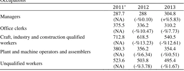
This could be traced to the sectoral composition of job losses in Portugal for this time as it affected the craft, industry and construction qualified workers5 the most, which, is a male dominant occupation.

(30)

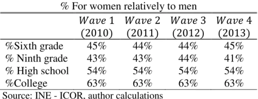
From Table A5 in Appendix we can see that, the probability of being unemployed in 2011, conditioned on being unemployed in 2010, was of approximately 70% for men and for women. In 2013, this probability increases to values of 81% and 78% for men and women, respectively. This suggests an increase of persistence in unemployment, which reinforces the need to study it, especially on the account of how high the unemployment rate was (17% of the active population was unemployed in 2013). Table 2 shows the distribution of the levels of education. This is meant to unveil the expected productivity for both genders, based only on education (excluding other relevant aspects, such as experience and training). From this we can see that women in the sample have a dominant presence on higher levels of education (high school and college), indicating higher expected productivity for women based only on education.

Table 2 –Distribution of levels of education % For women relatively to men

𝑊𝑎𝑣𝑒 1

(2010) 𝑊𝑎𝑣𝑒 2(2011) 𝑊𝑎𝑣𝑒 3(2012) 𝑊𝑎𝑣𝑒 4(2013)

%Sixth grade 45% 44% 44% 45% % Ninth grade 43% 43% 44% 41% % High school 54% 54% 54% 54% %College 63% 63% 63% 63%

In figures 1.a and 1.b, we consider three levels of experience, that differ with each age range. The first one is meant to represent higher attatchment to the labor market (in green), the second one that is meant to represent average attatchment (in the middle) and the last one represents low attatchment (red). For example, an individual who is aged between 20 to 30 years is expected to have, if his/her attatchment to the labor market is high, more than 5 years of experience or, if his/her attatchment is low, lower than 2 years of experience.

(31)

sample appear to have higher attatchment to the labor market. This conclusion comes from higher percentages for men, for each age range, in the levels of experience linked to higher attatchment, while women seem to focus on the middle levels of experience. Notwithstanding, when comparing 2013 to 2010, it appears as there has been a convergence, especially for the higher ranges of age. This is consistent with the idea that women are increasing their labor attatchment which in result will eventually reduce a gap in unemployment rates between genders.

Therefore, the data does replicate some of the results we expected from the literature survey, such as relatively lower labor attachment for women, with a convergence happening in this period of economic recession; higher presence in the lower levels of education for men; higher participation in part time employment for women relatively to

men; higher increase of men’s unemployment rate during a recession and persistence of

(32)

Market labor attatchment6

Figure 1.a –Relating age with experience7₍₂₀₁₀₎

Figure 1.b–Relating age with experience (2013)

6_{For the age range between 20 to 30 years old it was assumed that having two or less years of experience}

implied low attachment, while having more than five years implied high attachment; for the age range between 30 to 40 years old low attachment is having less than five years of experience while high attachment is having more than ten years of experience; for the age range between 40 to 50 years, low attachment is having less than ten years of experience while high attachment is having more than twenty years of experience; for the age range between 50 to 60 years old, low attachment is having less than twenty years of experience and high attachment is having more than forty years of experience.

(33)

5. THE RESULTS

In our model, we include the usual set of control variables that reflect individual characteristics and family variables that affect expected productivity, and also a fixed effect of time that aims to control for macroeconomic effects.

This section presents the main results obtained using the methodology developed in section 3 applied to the data described in section 4. It will be divided into three sub sections, the first sub section starts with the unrestricted random effects probit model, the second develops on the restricted model and presents the estimates for the average partial effects. Finally, the final section studies the persistence in unemployment.

5.1.RANDOM EFFECTS PROBIT MODEL

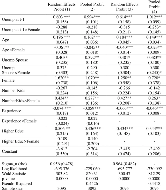
Estimates of panel data models for the probability of unemployment using both dynamic random effects probit (REP), modeled with the Mundlak device as in (8), and the pooled probit (PP), estimated for comparison purposes only, given the fact that its estimates are inconsistent, are given in Table A6 in Appendix. For these models the variables married

and the square of both experience and age were not included because they were highly insignificant. The variable married was replaced by the variable unemp spouse that is meant to reflect the employment status of the spouse of the individual which in result can control for family conditions.

(34)

of 10%. The only regressors which interact with the variable female that seem to have statistical significant (at a 10% level) between genders were age and numberkids. Notwithstanding, the differences between the models in Table A6 and Table A7, generally speaking, are not very significant, although the latter model beneficiates from higher efficiency that derives from being more parsimonious. All variables affect positively or negatively the probability of unemployment as expected from the literature survey, with the exception being the fact that age and unemployment condition of the

last period seemingly affect women’s probability of unemployment in a less negative

way than they affect men’s.

5.2. ESTIMATES OF AVERAGE PARTIAL EFFECTS

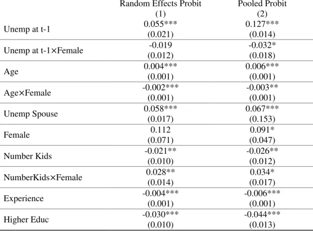
The contribution in the probability of unemployment of each exogenous variable considered is obtained through the estimation of the average partial effect (APE) of each variable averaged across the distribution of unobserved heterogeneity. Table 3 gives the average partial effects for each model.

(35)

Having an educational level assumed as high8_{, reduces the overall probability of}

unemployment in 0.030 pr.p. while having a spouse that is unemployed raises it in 0.058 pr.p.. The first result is consistent with the literature, as it was expected that individuals with higher education would appear to have higher levels of productivity to employers. For the second result, there was no relevant literature that could explain this positive association between the unemployment status of an individual and of his or her spouse. Therefore, this comes as an especially interesting result that could be further developed in the future, perhaps as an association between higher probability of unemployment and employment unstableness of the household. This could also represent how most economic crisis affect the population differently, resulting in higher levels of inequality. The number of kids has different effects on the probability of unemployment when we consider both genders. When comparing a woman with the same number of kids as a man, while controlling for all other covariates, she will, on average, have a higher probability of being unemployed of 0.028 pr.p..

The positive and significant coefficient of the lag of the dependent variable suggests that there is persistence in unemployment. Therefore, our results provide favorable evidence that past unemployment raises the probability of current unemployment. For the considered time period, women seem to suffer less from this situation. Although surpassing the usual 10% significance level, with a p-value of 10,7%, the interaction between female and the lag of the dependent variable reaches an APE of -0.019 pr.p. in the REP model. Notwithstanding, if we consider the PP model, this APE turns out to be statistically significant, reducing the effect of unemployment persistence for women in 0.032 pr.p..

(36)

Table 3 – Average partial effects

Random Effects Probit (1)

Pooled Probit (2) Unemp at t-1 0.055***

(0.021)

0.127*** (0.014) Unemp at t-1×Female -0.019

(0.012)

-0.032* (0.018)

Age 0.004***

(0.001)

0.006*** (0.001) Age×Female -0.002***

(0.001)

-0.003** (0.001) Unemp Spouse 0.058***

(0.017)

0.067*** (0.153)

Female 0.112

(0.071)

0.091* (0.047) Number Kids -0.021**

(0.010)

-0.026** (0.012) NumberKids×Female 0.028**

(0.014)

0.034* (0.017) Experience -0.004***

(0.001)

-0.006*** (0.001) Higher Educ -0.030***

(0.010)

-0.044*** (0.013)

Notes:

1. Standard errors are in brackets. For both models the standard error was computed with the Delta Method.

2. Significance levels: *10%, **5%, ***1%.

3. The APE of the variable Unemp at t-1×Female has a p-value of 10,7% for the RE model.

4. The APE of the variable Female has a p-value of 11,2% for the RE model.

(37)

the literature related to this topic, unemployment persistence can reflect increases in the natural rate of unemployment, i.e., can reflect increases in the long run equilibrium of the unemployment rate. Consequently, if the unemployment rate has been persistently high in result of an increase in the long-term equilibrium unemployment rate, labor market policies should focus on structural labor reforms rather than only focusing on increasing short term employment. Because this was a period marked by high unemployment rates and, simultaneously, a reduction in public spending, the lack of policies aimed to fix this crisis-aggravated problem could eventually translate into a slow adjustment of the unemployment rate that might actually never achieve the same level as in the period before the crisis. Therefore, labor market reforms, especially in the form of creating stable employment and in the form of increasing human capital of long term unemployed individuals, need to take place in order to prevent the results that come from permanently higher unemployment rates.

(38)

affected male dominant industries the most and that men might be more reluctant to accept any job, especially if it’s not in the field of their previous occupation.

6. CONCLUSIONS AND SUGGESTIONS FOR FURTHER RESEARCH The present work provides some answers on important questions regarding gender discrimination and unemployment persistence in the Portuguese labor market. We estimated a binary panel data model for the probability of unemployment that simultaneously controls for unobserved individual heterogeneity. This unobserved heterogeneity, in this context, could represent important individual characteristics that are not observable, such as individual ability and unobserved discrimination, both taste-based and statistical discrimination.

Our results suggest that there is evidence of higher probabilities of unemployment for women, relatively to men, in spite of women having stronger presence in higher levels of education. Notwithstanding, it appears that the economic crisis helped closing the gender gap in the probability of unemployment, with the unconditional unemployment rate of men surpassing women’s, replicating some empirical evidence which found that,

in periods of economic recession, men’s unemployment rate rises faster than women’s.

This could reflect the effect of higher female labor force attachment9 fueled by higher financial necessities and labor instability, a result from the economic crisis affecting Portugal during this time. Higher education and experience appear to have negative effects on the probability of unemployment, contributing to its reduction. Thus, the importance of human capital in reducing the probability of unemployment is reinforced. By controlling for ability, which is assumed to be included in the unobserved heterogeneity, these human capital effects become independent of differences in ability,

(39)

which strengthens the idea that the attainment of higher levels of education and of higher labor attachment are reliable signals of high marginal productivity to employers. Both age and the number of kids seem to influence the probability of unemployment differently between genders, with the increase of the number of kids raising the probability of unemployment for women, while reducing it for men. This is consistent with the theory that taking care of kids is still a job predominately done by women. In particular, having kids might affect women’s presence in the labor market in a twofold way: by signaling employers that women might need to leave work more often or by

reducing women’s desire in full time work experience. Some policies regarding this particular result should take place, as childbearing is especially important for Portugal, a country that has been suffering by the complications that arise from population ageing, in particular hindering the foundation of social security. This could be done e.g. by reducing the non-wage cost of labor, in particular by offering day care benefits to newly parents and by forcing both genders to take an equal amount of days in parental leave. When we tried to control for discrimination using a fixed effect for women, we obtained strong statistical evidence that it increases women’s probability of unemployment. This indicates that labor reforms should focus on trying to reduce both taste-based and statistical discrimination, e.g. focusing on attaining gender parity in occupations, as it

may change society’s perception on gender roles by not socially restricting particular

(40)

-gender-dominated” industry. In the long run, if a parity is attained for most occupations then,

eventually, it could translate into a change in both occupational and educational gender segregation, as well as into eliminating all statistical discrimination that come from distorted perceptions of expected productivity based on gender.

We were also able to find strong state dependence effects with respect to previous unemployment incidence, during this period of high unemployment in Portugal. This finding is consistent with the theory that previous unemployment experience has a sizeable impact on future employment. It can also be a result from a higher structural unemployment rate, which suggests that, despite the focus on fiscal consolidation, Portugal is concurrently in need of deep labor reforms that aim to provide better conditions for individuals that want to work. Therefore, if employment instability has such high implications on future employment, labor policies should focus on offering higher assistance in job-search and training programs to individuals who have been unemployed for some time. Hence, it would be possible to contradict the trend of human capital depreciation and could eventually lead to higher employability.

(41)

occupation and women in other occupations. Some other relevant aspects could be studied in order to reveal the extent that discrimination can have on the labor market, such as educational segregation, e.g. the impact that choosing a STEM field of

(42)

REFERENCES

Ahmad, N. (2014). State dependence in unemployment. International Journal of Economics and Financial Issues, 4(1), 93.

Aigner, D. J., & Cain, G. G. (1977). Statistical theories of discrimination in labor markets. ILR Review, 30(2), 175-187.

Albanesi, S., & Şahin, A. (2013). The gender unemployment gap. Staff Report, Federal Reserve Bank of New York, No. 613.

Arrow, Kenneth (1973). The theory of discrimination, in: O. A. Ashenfelter and A. Rees, (Eds.) Discrimination in labor markets, Princeton, N.J.: Princeton University Press, pp. 3-33.

Azmat, G., Güell, M., & Manning, A. (2006). Gender gaps in unemployment rates in OECD countries. Journal of Labor Economics, 24(1), 1-37.

Arulampalam, W., Booth, A. L., & Taylor, M. P. (2000). Unemployment persistence.

Oxford Economic Papers, 52(1), 24-50.

Arulampalam, W. (2001). Is unemployment really scarring? Effects of unemployment experiences on wages. The Economic Journal, 111(475), 585-606.

Arulampalam, W., Gregg, P., & Gregory, M. (2001). Unemployment scarring. The Economic Journal, 111(475), 577-584.

Becker, Gary S. (1971). The economics of discrimination, 2ªEd. Chicago: The University of Chicago Press. (Original edition, 1957.)

Bielby, W. T., & Baron, J. N. (1986). Men and women at work: Sex segregation and statistical discrimination. American Journal of Sociology, 91(4), 759-799. Blau, F. D., & Kahn, L. M. (1997). Swimming upstream: Trends in the gender wage

(43)

Cejka, M. A., & Eagly, A. H. (1999). Gender-stereotypic images of occupations correspond to the sex segregation of employment. Personality and Social Psychology Bulletin, 25(4), 413-423.

Eagly, A. H., & Karau, S. J. (2002). Role congruity theory of prejudice toward female leaders. Psychological Review, 109(3), 573.

Elmeskov, J., & MacFarlan, M. (1993). Unemployment persistence. OECD Economic Studies, 57-57.

Gauchat, G., Kelly, M., & Wallace, M. (2012). Occupational gender segregation, globalization, and gender earnings inequality in US metropolitan areas. Gender & Society, 26(5), 718-747.

Gottfredson, L. S. (1981). Circumscription and compromise: A developmental theory of occupational aspirations. Journal of Counseling Psychology, 28(6), 545. Jackman, R. (2002). Determinants of unemployment in western Europe and possible

policy responses. Paper presented at UNECE’s 5thSpring Seminar Geneva, 1-38.

Kögel, T. (2004). Did the association between fertility and female employment within OECD countries really change its sign?. Journal of Population Economics, 17(1), 45-65.

Manning, A., & Swaffield, J. (2005). The Gender Pay Gap in Early Career Wages Growth. CEP Discussion Paper, 679.

(44)

Petrongolo, B. (2004). Gender segregation in employment contracts. Journal of the European Economic Association, 2(2-3), 331-345.

Phelps, E. S. (1972). The statistical theory of racism and sexism. The American Economic Review, 62(4), 659-661.

Statistics Portugal (2011). Statistical Yearbook of Portugal 2010, 30th September 2011. Portugal: Statistics Portugal Available at: https://www.ine.pt

Şahin, A., Song, J., & Hobijn, B. (2010). The unemployment gender gap during the 2007 recession. Current Issues in Economics and Finance, 16 (2), 1–7 (Federal Reserve Bank of New York).

Spence, M. (1973). Job market signaling. The Quarterly Journal of Economics, 87(3), 355-374.

Wright, D. B., Eaton, A. A., & Skagerberg, E. (2015). Occupational segregation and psychological gender differences: How empathizing and systemizing help explain the distribution of men and women into (some) occupations. Journal of Research in Personality, 54, 30-39.

Wooldridge, Jeffrey M. (2010), Econometric analysis of cross section and panel data, The MIT Press, Cambridge, England.

(45)

(46)

APPENDIX

Table A1 – Variable definitions and expected effects

Variable Description Expected effect Unemp Unemployed at time of the interview

(ILO definition)

-Age Age of the individual Positive Unemp Spouse Equals 1 if the spouse is unemployed Ambiguous Female Equals 1 if the individual is a woman Positive Number Kids Number of kids of the individual who

were also in the original database Positive Experience Number of years in paid work Negative Higher Educ Equals 1 if the individuals has a degree

equivalent to high school or higher Negative

Notes:

1. Pooled data for 4 waves of the ICOR (2010-2013) 2. Sample size = 3096

(47)

Table A2 – Descriptive Statistics of the variables

Variable Mean Std. Deviation Min Max

Unemp 0,150 0,357 0 1

Age 42,375 10,474 17 66

Unemp Spouse 0,101 0,302 0 1

Female 0,500 0,500 0 1

Number Kids 0,461 0,713 0 5

Experience 23,610 12,335 0 54

Higher Educ 0,386 0,487 0 1

Notes:

1. Pooled data for 4 waves of the ICOR (2010-2013) 2. Sample size = 3096

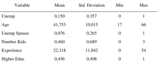
Table A3 – Descriptive Statistics of the variables for women

Variable Mean Std. Deviation Min Max

Unemp 0,150 0,357 0 1

Age 41,753 10,015 17 66

Unemp Spouse 0,076 0,265 0 1

Number Kids 0,460 0,689 0 3

Experience 22,318 11,842 0 54

Higher Educ 0,456 0,498 0 1

Notes:

(48)

Table A4 – Employed population according to main occupation (ISCO-08) in thousands (%∆)

Occupations

2011∗ ₂₀₁₂ ₂₀₁₃

Managers 287.7

(NA)

288 (-%0.10)

304.8 (+%5.83)

Office clerks 375.5

(NA)

336.2 (-%10.47)

310.2 (-%7.73) Craft, industry and construction qualified

workers 712.8 (NA) 618.5 (-%13.23) 540.5 (-%12.61) Plant and machine operators and assemblers 380.3

(NA)

356.2 (-%6.34)

354.4 (-%0.51) Unqualified workers 523.6

(NA) 503.8 (-%3.78) 495.4 (-%1.67) Notes:

1. Data from Statistics Portugal, Labor Force Survey 2. *Values of ISCO-08 not available for 2010

Table A5 – Transition probabilities (from unemployment or employment to unemployment)

2011 2012 2013

Male

𝑈𝑛𝑒𝑚𝑝𝑙𝑜𝑦𝑒𝑑 𝑡−1= 0 0.0552 0.0708 0.0495

𝑈𝑛𝑒𝑚𝑝𝑙𝑜𝑦𝑒𝑑 𝑡−1= 1 0.6957 0.8431 0.8060

Total 0.1308 0.1718 0.1795

Female

𝑈𝑛𝑒𝑚𝑝𝑙𝑜𝑦𝑒𝑑 𝑡−1= 0 0.0431 0.0517 0.0547

𝑈𝑛𝑒𝑚𝑝𝑙𝑜𝑦𝑒𝑑 𝑡−1= 1 0.6949 0.6909 0.7818

Total 0.1432 0.1432 0.1589

Notes:

1. The total is the proportion of individuals who were unemployed in the sample for the correspondent year

2. 𝑈𝑛𝑒𝑚𝑝𝑙𝑜𝑦𝑒𝑑 _𝑡−1= 0 has the proportion of the individuals who are unemployed in 𝑡 given that they were employed in 𝑡 − 1

(49)

Table A6– Panel data models for the probability of unemployment Random Effects Probit (1) Pooled Probit (2) Random Effects Probit (3) Pooled Probit (4)

Unemp at t-1 0.603 ***

(0.158) 0.994*** (0.101) 0.614*** (0.158) 1.012*** (0.099) Unemp at t-1×Female -0.288

(0.213) -0.218 (0.148) -0.315 (0.211) -0.253* (0.145)

Age 0.196 ***

(0.047) 0.162*** (0.036) 0.184*** (0.045) 0.149*** (0.034)

Age×Female -0.061**

(0.028) -0.045** (0.018) -0.040*** (0.014) -0.023** (0.009)

Unemp Spouse 0.403*

(0.235) 0.392** (0.180) 0.401* (0.235) 0.383** (0.180) Unemp

Spouse×Female

0.375 (0.303) 0.290 (0.248) 0.380 (0.304) 0.300 (0.245)*

Female 1.620**

(0.738) 1.070** (0.106) 1.250** (0.558) 0.720* (0.378)

Number Kids -0.267

(0.224) -0.145 (0.156) -0.266 (0.224) -0.142 (0.154) NumberKids×Female 0.434**

(0.210) 0.277** (0.136) 0.427** (0.208) 0.263* (0.138)

Experience -0.074 ***

(0.018) -0.059*** (0.012) -0.063*** (0.012) -0.046*** (0.008) Experience×Female 0.022

(0.024)

0.022

(0.016) - -

Higher Educ -0.506 **

(0.215) -0.436*** (0.163) -0.434*** (0.148) 0.344*** (0.103) Higher Educ×Female 0.109

(0.291)

0.140

(0.209) - -

Constant -3.612

(0.530) -2.704 (0.314) -3.415 (0.474) -2.492 (0.286)

Sigma_u (rho) 0.956 (0.478) - 0.964 (0.482) -

Log likelihood -695.376 -729.060 -695.777 -730.092

Wald Statistic 303.82 820.31 300.47 812.29

p-value 0.0000 0.0000 0.0000 0.0000

Pseudo-Rsquared - 0.4426 - 0.4418

Sample size 3095 3095 3095 3095

Notes:

1. Standard errors are in brackets. For the Pooled Probit model we computed cluster-robust standard errors.

2. All models contain year dummies for 2011, 2012 and 2013 and, additionally, controls as specified by the Mundlak device in equation (6).

3. Significance levels: *10%, **5%, ***1%.

Master in Applied Econometrics and Forecasting

Lisbon School of Economics & Management