Job Destruction in the Theory of Unemployment

Review of Economic Studies (1994) 61, 397-415 0034-6527/94/00200397$02.00

?3 1994 The Review of Economic Studies Limited

Job

Creation

and

Job

Destruction in

the

Theory

of

Unemployment

Northwestern University and

CHRISTOPHER A. PISSARIDES London School of Economics

First version received December 1991 ;final version accepted December 1993 (Eds.)

In this paper we model a job-specific shock process in the matching model of unemployment with non-cooperative wage behaviour. We obtain endogenous job creation and job destruction processes and study their properties. We show that an aggregate shock induces negative correlation between job creation and job destruction whereas a dispersion shock induces positive correlation. The job destruction process is shown to have more volatile dynamics than the job creation process. In simulations we show that an aggregate shock process proxies reasonably well the cyclical behaviour of job creation and job destruction in the United States.

1. INTRODUCTION

Recent microeconomic evidence from the U.S. and other countries has shown that largejob creation and job destruction flows co-exist at all phases of the business cycle.' Individual establishments have diverse employment experiences even within narrowly defined sectors and regardless of the state of aggregate conditions. In this paper we develop a model of endogenous job creation and job destruction and incorporate it into the matching approach to equilibrium unemployment and wage determination. In our model, establishments have diverse experiences because of persistent idiosyncratic shocks. We examine the implications of the model for the processes of job creation and job destruction and for the aggregate behaviour of unemployment and job vacancies.

The economy we examine has a continuum of jobs that differ with respect to values of labour product. Each job is designed to produce a single unit of a variation on a common product. Each variation is unique to the job and commands a relative price that is subject to idiosyncratic risk, due to either taste or productivity shocks. A key assumption is that investment is irreversible, so an existing job cannot switch the variation of its product once the job has been created. But before creation, technology is fully flexible and the firm can choose the variation of its product. We model the idiosyncratic risk for existing jobs as a jump process characterized by a Poisson arrival frequency and a drawing

1. For the U.S. see Leonard (1987), Davis and Haltiwanger (1991) and Blanchard and Diamond (1990), for Germany Boeri and Cramer (1991) and for Italy Contini and Revelli (1988).

from a common distribution of relative prices. Large negative shocks induce job destruc- tion but the choice of when to destroy the job is the firm's.

Job creation depends on the information available to potential employers. In empirical work two sources of new jobs are usually given, existing firms and new entrants. Most new job creation over the cycle is by existing firms; in Davis and Haltiwanger's (1990, 1991) study of U.S. manufacturing establishments, firms three years or under account for only about 18% of total job creation. Existing firms have good information about the profitability of new differentiated products within their sectors, so a natural assumption to make is that new jobs are more productive than existing ones. We take this assumption to its extreme and assume that newly-created jobs are the most profitable in the market. An assumption of this kind is less easily justified if job creation is by new entrants, a route that we do not pursue here.2

Following on from our assumption that idiosyncratic risk is job-specific, we also model the matching process as taking place between individual job vacancies and unem- ployed workers, rather than between multiple-job firms and workers. Consequently, with the productivity of new jobs at the upper support of the distribution and a large number of potential jobs, there is a zero-profit condition for a new job vacancy that can produce the most highly valued product in the market. Given our assumption of constant returns in the matching technology, zero expected profit on a new vacancy is equivalent to a marginal productivity condition for any job -that produces the most highly priced product variation.3

Wages are the outcome of a bilateral bargain that takes place when unmatched jobs and workers meet and is revised continuously in the face of productivity shocks. An equilibrium is a time path for the number of job/worker matches (and hence employment) implied by the matching law and rational non-cooperative behaviour by individual workers and employers. We study both the aggregate steady state of the equilibrium deterministic process and the dynamic adjustments in response to persistent aggregate shocks.

In the next section, various concepts and notation are defined. Following that, in Section 3, the implications of micro and macro parameters for job creation and job destruction and for steady-state vacancy and unemployment levels are derived. The effects of persistent "cyclical" changes in the common macro and micro parameters are studied in Section 4. Section 5 simulates an example of the model and shows that our model solutions proxy reasonably well the observed behaviour of job creation and job destruction found in the U.S. data.

2. CONCEPTS AND NOTATION

Each firm has one job that can be in one of two states, filled and producing or vacant and searching. Jobs that are not actively producing or searching are destroyed. Following the empirical literature, we say that job creation takes place when a firm with a vacant job and a worker meet and start producing; opening a new job vacancy is not job creation,

2. New entrants have on average shorter lives than existing firms, which would contradict our assumptions. In a recent paper related to ours, Caballero and Hammour (1991) study the cyclical behaviour of job creation and job destruction in a vintage model of embodied technical change by assuming that new entrants adopt the most advanced technology. Another recent paper that addresses the question of cyclical changes in job creation and job destruction is by Bertola and Caballero (1991), where existing firms move probabilistically between two states, good and bad, and jobs form after a matching process.

MORTENSEN & PISSARIDES JOB CREATION AND DESTRUCTION 399

though we might refer to it as creating a job vacancy. Job destruction takes place when a filled job separates and leaves the market.

Similarly, workers can be either unemployed and searching or employed and produc- ing. We do not consider search on the job to avoid complicating the model, though our assumptions on technology and wages imply that there are incentives to search on the job, unless the cost of on-the-job search is too high.4 Wages are chosen so as to share at all times the surplus from a job match in fixed proportions. The worker's share is

fl.5

Consequently, more productive jobs offer higher wages and since job vacancies are charac- terized by the best technology in the market, new jobs offer the highest wage.

Each job is characterized by a fixed irreversible technology and produces a unit of a differentiated product whose price is p + uc. This price can be referred to as either the productivity of the job or simply as its price. p and a are common to all jobs whereas ?

is job specific. p is an aggregate component of productivity that does not affect the disper- sion of prices. The parameter a reflects dispersion, an increase in a representing a symmet- ric mean preserving spread in the job-specific shock distribution or equivalently an increase in price variance.

The process that changes the idiosyncratic component of price is Poisson with arrival rate A. When there is change, the new value of ? is a drawing from the fixed distribution

F(x), which has finite upper support cu and no mass points. Without further loss of generality, F(x) can be endowed with zero mean and a unit variance so that a is the standard deviation of the job-specific component au.6

Modelling the arrival process as Poisson implies persistence in job-specific shocks, but conditional on change, the firm's initial conditions do not affect its next price. Exogen- ous events that affect the persistence or distribution of idiosyncratic shocks (micro shocks) shift A and a respectively. Events that affect the productivity of all jobs by the same amount and in the same direction (macro shocks) are reflected in changes in the common price component p.

Firms create jobs that have value of product equal to the upper support of the price distribution, p + asu. Once a job is created, however, the firm has no choice over its productivity. Thus, job productivity is a stochastic process with initial condition the upper support of the distribution and terminal state the reservation productivity that leads to job destruction. Both job creation and job destruction are costless, so we can either assume

that the firm can choose its technology after it is matched to a worker or before it is matched, with identical results. In the latter case, when a vacancy is hit by an idiosyncratic shock it exits and re-enters at the best technology, so all active vacancies can produce the product variation that commands price p + Eu. Filled jobs, however, do not always exit when they are hit by shocks, because there is a cost of recruiting, modelled as a per-unit cost of maintaining a vacancy, c. Existing filled jobs are destroyed only if the idiosyncratic component of their productivity falls below some critical number Ed < u. Therefore, the

rate at which existing jobs are destroyed is AF(Ed).

The rate at which vacant jobs and unemployed workers meet is determined by the homogeneous-of-degree-one matching function m(v, u), where v and u represent the num- ber of vacancies and unemployed workers respectively, normalized by the fixed labour

4. On-the-job search introduces new results by drawing the distinction between worker flows and job flows. Here the two flows are identical. The results that we highlight in this paper are not affected by the absence of on-the-job search. See Mortensen (1993).

5. For motivation and discussion of this wage rule, which is the one most frequently used in the search literature, see Diamond (1982), Mortensen (1982) and Pissarides (1990).

force size. Since vacancies offer the highest wage no job seeker turns down a vacancy, so the transition rate for vacancies is q = m(v, u)/v = m( 1, u/v), with q'(v/u) < 0 and elasticity strictly between -1 and 0. The rate at which seekers meet vacancies is vq/u=m(v/u, 1). Job creation is defined by the number of matches, m(v, u) = vq(v/u).

The unknowns of the model are the number of job vacancies v and unemployment u, which determine, through the matching technology, job creation, and the critical value for the idiosyncratic component of productivity, Ed, that induces job destruction.

3. STEADY STATES

The assumptions that vacancies cost c per unit time and that jobs are created at the upper end of the price distribution imply

r V= -c + q(vlu) [A6u) -VI, (1

where V and J(e) are respectively the asset values of a vacancy and of a filled job with idiosyncratic component E. Job creation until the exhaustion of all rents implies

rV=0. (2)

In order to determine the productivity-contingent wage, w(?), we denote the worker's

asset value from a match with idiosyncratic component ? by W(E) and his asset value

from unemployment by U. Total match surplus is

S(e) = J(A) + W(E)- U. (3)

The wage is set to split the surplus in fixed proportions at all times, so

W(C) -U= ,BS( E), (4)

where

fi

Since firms have the option of closing jobs at no cost, a filled job continues in operation for as long as its value is above zero. Hence, filled jobs are destroyed when a productivity shock x arrives that makes J(x) = (1 - P)S(x) negative. For any realization ?, J(E) solves,

rJ(E)=p+uc-w(e)+2A(1-f,) Jr{max [S(x),0]-S(e)}dF(x). (5)

Similarly, the value of the job to the worker solves,

rW(c)=w(e)+2A3 f {max [S(x), 0]-S(e)}dF(x). (6)

Finally, the present value of income of an unemployed worker is defined by

rwU= (vqlu)r

b

[

MORTENSEN & PISSARIDES JOB CREATION AND DESTRUCTION 401

Adding up the value expressions (5)-(7) and making use of the sharing rule (4), we get,

(r+)A)S(e) =p+ as-b+ A {max [S(x), O]dF(x)-f(vq/u)S(Eu). (8) Since S(E) is monotonically increasing in e, job destruction satisfies the reservation prop- erty. There is a unique reservation productivity Ed7 that solves J(ed) = ( - P)S(Ed) = 0,

such that jobs that'get a shock 6< Ed are destroyed. This condition and the fact that

S'(e) = a/(r + A) imply, after integration by parts,

rEU

(r + A)S(E) =p + ag- b + A _{S'(X) [I- F(X) ]dx - P(vqlu) S(Eu)}

Ed

=p+ Ug-b+ ? f _{[1 -F(x)]dx-P(vq/u)S(Eu).} (9)

Since S(Eu)=J(A6)/(0 -f) and S(ed)=0, (1), (2) and (9) imply,

PiC v c

p+CTSd=b+

a

IflOu r-TA Ed

This is one of the key conditions of the model. It gives the reservation productivity in terms of the ratio of vacancies to unemployment and the parameters of the model, so, with knowledge of v/u, it can be used to derive the job destruction rate, AF(ed).

The left-hand side of (10) is the lowest price acceptable to firms with a filled job. This is less than the opportunity cost of employment because of the existence of a hiring cost. The opportunity cost of employment to the worker is the value of leisure b plus the expected gain from search, which in equilibrium is equal to the second term on the right- hand side of (10). The third term is a measure of the extent to which the employer is willing to incur an operational loss now in anticipation of a future improvement in the value of the match's product, i.e., it is the option value of retaining an existing match. That this is positive is indicative of the existence of "labour hoarding" at low price realizations.8

Holding the v/u ratio constant, it is easily established by differentiation that the reservation productivity gd decreases with the difference between the aggregate productivity parameter, p, and the value of leisure, b. It is also easily established that because the decrease in gd increases the option value of a job, the increase in p reduces the reservation

price p + USd: the range of prices observed at higher common price expands.

The term flcv/(l - f)u stands for the expected gain from search, which, without on- the-job search, has to be given up when the worker accepts a job. A higher expected return from search increases the opportunity cost of employment and so leads to higher Ed and

to more job destruction.

An increase in A increases the option value of a job because job-specific product values are now less persistent. So, at higher A a job experiencing a bad shock is less likely to be destroyed. In contrast, a higher discount rate, r, reduces future profitability at all

7. The reservation productivity, or price, is obviously p + a6d . We refer to ed as the reservation productivity

to avoid the more cumbersome reservation value of the idiosyncratic component of productivity.

8. It can easily be checked that if c=O, J(eu) =0 from (1) and (2) and so 8d= Eu: given the exogeneity of

prices, and so reduces the option value of waiting for an improvement. Thus, given v/u, A decreases Ed and r increases it.

The relation between the variance of the idiosyncratic shock, a, and Ed is in general

ambiguous. Higher a implies that the more profitable jobs become even more profitable but less profitable jobs suffer a price reduction. Since the price of operational jobs, however, is given by p + as for Ed ? e _ Eu, the higher a necessarily implies a general improvement

in the productivity of existing jobs, though some of the existing jobs may become less profitable. Generally speaking, the reservation productivity is higher when a is higher, increasing the rate of job destruction, when the marginal job is less profitable at the higher a. Differentiating (10) with respect to a gives, for given v/u,

8gd (r+2)/u p-b- fC (11)

Oa r+AF(Ed) 1-fl u

Given v/u, Ed increases in a if p exceeds the opportunity cost of employment. In this case

(10) implies that Ed is a negative number, so the productivity of the marginal job is lower

at higher a. Since, however, a improves the option value of the job, the cutoff point where higher a implies more job destruction is not Ed = 0 but some Ed < 0

It is reasonable to assume that p exceeds the opportunity cost of employment. First, it implies that a labour market equilibrium exists at all (non-negative) values of a. Second, it implies that not all prices in the truncated price distribution, with range p +a Ed to

p + usu, increase when a increases, making a a more appealing measure of dispersion in an empirical price distribution. In the discussion that follows we assume that the conditions for a positive effect of a on gd are satisfied.

The solution for the other two unknowns of the model, vacancies and unemployment, is obtained from (1) and (2) and the steady-state condition for unemployment. To write (2) in a more convenient form, note that (9) implies,

S() - S(Ed) = ( d) (12)

r+). Therefore, (1)-(4) imply

(aq I_

r+)

I_6U(Eu - Sd)

Equation (13) is the job creation condition and, with (10), uniquely determines v/u and gd-

The joint determination of v/u and Ed iS illustrated in Figure 1. The curve labelled

JD represents the job destruction condition (10) and the curve JC the job creation condi- tion (13). JD slopes up because at higher v/u the opportunity cost of employment is higher, so there is more job destruction. JC slopes down because at higher Ed job destruction is

more likely, so there is less creation.

As earlier explained, for given v/u an increase in common price p or a decrease in the exogenous cost of employment b shifts JD to the left, so the equilibrium v/u increases and the equilibrium gd decreases. An increase in A shifts JD to the left and JC down, so it decreases Ed. The diagram gives an ambiguous effect on v/u but differentiation of (10)

MORTENSEN & PISSARIDES JOB CREATION AND DESTRUCTION 403

V/U JD

Jc

Ed

FIGURE 1

The joint determination of v/u and 8d

The effect of disperion, a, is to increase v/u at given Ed and so shift JC up. It also

increases Ed at given v/u, so it shifts JD to the right. The overall effect is an increase in

E.9 As with A, the diagram gives an ambiguous effect on v/u but it can be established by

differentiation that v/u unambiguously increases in a, regardless of the relation between p and b (see the Appendix).

The final equation of the model is the steady-state condition for unemployment, or Beveridge curve. The flow out of unemployment equals the flow into unemployment at points on the curve. The endogenous job separation rate is AF(ed) and the job matching rate per unemployed worker is m(v/u, 1), so the equation for the Beveridge curve is

U AF(Ed) (14)

AF(ed)+m(v/u, 1)

It is conventional to draw the Beveridge curve convex to the origin in vacancy- unemployment space, but differentiation of (14) shows that in this model there is an ambiguity about the curve's precise shape. On the one hand, higher vacancies imply more job matchings, so unemployment needs to be lower for stationary matching rate. On the other hand, higher vacancies also imply more job destruction, through the effects of v/u on Ed, so unemployment needs to be higher to maintain stationary job destruction rate.

Thus, whether the curve slopes down or not depends on the relative strength of each effect. In models without an endogenous job destruction rate only the former (matching) effect is present and in that case the homogeneity of the matching function ensures that the Beveridge curve is convex to the origin. Since empirically that shape is more plausible, we shall assume here that the matching effect on the Beveridge curve dominates the job destruction effect and the curve slopes down. This is shown in Figure 2.

In order to obtain the steady-state equilibrium vacancy and unemployment combina- tion we draw a line through the origin to represent the equilibrium solution for v/u, obtained from (10) and (13) and illustrated in Figure 1. We refer to this as the job creation

9. The Appendix shows that the condition for a positive effect of a on Ed, when variations in v/u are

v

Job creation

Beveridge

curve

u

FIGURE 2

Equilibrium vacancies and unemployment

condition. Given the reservation productivity, equilibrium vacancies and unemployment are given at the intersection of the job creation condition and the Beveridge curve.

The job creation flow is m(v, u) and the job destruction flow is AF(ed)(I - u). The analysis that follows derives the initial impact of parameter changes on each conditional on current unemployment, u. Obviously, unemployment eventually adjusts to equate the two in steady state. Note that an increase in job creation rotates the job creation condition up in v/u space while an increase in job destruction shifts the Beveridge curve out.

A positive net aggregate productivity shock, represented by either an increase in p or a fall in b, increases v/u and decreases Ed, so it rotates the job creation condition in Figure

2 up and shifts the Beveridge curve in. In other words, job creation increases and job destruction decreases in response to a positive macro shock. Eventually, unemployment falls but the effect on vacancies is ambiguous. The differences between these implications and those of the pure matching model is the shift in the Beveridge curve and the resulting ambiguity of the vacancy effect.

An increase in the variance of the idiosyncratic shock increases both job creation and job destruction. Its effects in vacancy-unemployment space are to shift the Beveridge curve out and rotate the job creation line up. Equilibrium vacancies increase but the effect on unemployment is ambiguous.

In contrast, a reduction in persistence, shown by an increase in A, rotates the job creation condition down and shifts the Beveridge curve out, given the reservation produc- tivity. The effect on job destruction is mitigated and can be reversed in principle, thus not shifting the Beveridge curve, by the reduction in the reservation productivity induced by an increase in shock frequency. Whether or not a sign reversal occurs depends critically on the magnitude of the discount rate, r, and on the extent of the dispersion in the shock, a, as the effect of A on the reservation productivity falls with either (the direct effect tends to zero as r-+0 or c -+0) by virtue of (10).

4. CYCLICAL SHOCKS

MORTENSEN & PISSARIDES JOB CREATION AND DESTRUCTION 405

p takes two values, a high value p* and a low value p, according to a Poisson process with rate p. The Poisson process captures the important feature that characterize cyclical shocks, a positive probability less than one that boom or recession will end within a finite period of time. We also discuss the cyclical implications of changes in the disperion of the job-specific shocks. The purpose of this analysis is to bring out the differences between the steady-state equilibrium studied so far and the equilibrium obtained when there is anticipation of aggregate productivity change.

In the model of Section 3 the steady-state equilibrium solutions for Ed and v/u for a

given price p are given by equations (10) and (13). Since in modelling the exhaustion of rents from new jobs both Ed and v were treated as forward-looking jump variables, and

history did not matter in either of the expressions derived for them, the solutions for the two variables jump between the steady-state equilibrium pair Ed and v/u on the one hand

and Ed* and (v/u)* on the other, as price jumps between p and p*. In contrast, unemploy-

ment is a sticky variable, since it changes according to the laws governing the matching technology. The differential equation describing the evolution of unemployment for any given price p is

u=(1-u)AF(ed)-um(v/u, 1). (15)

The steady-state analysis leads us to expect that since p* >p, E* < Ed and (v/u)* >

v/u. Therefore, when price drops from p* to p, some marginal jobs are immediately destroyed and some vacancies close down. In contrast, when price increases from p to p*, new vacancies are opened up but nothing happens to employment on impact. This asymme- try will turn out to have an important cyclical implication for the behaviour of the job creation and job destruction rates.

As before, jobs are destroyed whenever their value falls below zero. Equations (1)- (4) of the steady-state model still hold for each p. The expressions for the returns from a filled job, employment and unemployment, (5)-(7), need to be modified to reflect the fact that common price may now change. Moving directly to the value equation for the job's net surplus (8), denoting by S*(e) the surplus from a filled job when common price is p*, and noting that if S(e) <0 the job is destroyed, (8) becomes,

(r + A + p)S(E) =p + ae-b + A J4 S(x)dF(x)- 13(vq/u)S(Eu) + p S*(4E) E >-Ed,

(16)

rgu

(r+2A+p)S*(E)=p*+ae-b+2A S(x)dF(x) - (vq/u)*S*(eu)+pS(e) _Ed,

Ed

(17)

(r.+A+P)S*(E)=p + u-b+ { S* (x)dF(x)1-3(vq/u)* S *(u) d> eed.

(18) Equation (16) gives the surplus from the job when price is at the low value p. It is indentical to (8), except that the possibility of the price changing form p to p*, at rate P, adds the term p[S*(E) - _{S(E)] to the net return from the job. Equation (17) is the price equal to}

the high value p*. When e>_ Ed, the job survives when the price drops from p* to p;

therefore, the net return from the job when the transition is expected falls by the expected capital loss p[S*(E) - _{S(E)]. In (18), price is again at p*, but now the job's idiosyncratic}

p, so the expectation of the price change leads to the loss of the job's surplus without any gain (for these jobs and by the definition of Ed, S(E) <0).

The reservation shock 4 solves S*(e*)=0. The relevant expression for S*(Ed) is (18), where by differentiation, 8S*(E)/9E= u/(r+A+p) for Ed> Ed * and, from (16)

and (17), OS*(E)/OE= a/(r+ A) for e? Ed. Hence, integration of (18) by parts gives,

(r+ A+ p)S*(e) =p* + sE-b -,(vqlu)*S*(,U)

('rEd ATo - U

+ [ [I-F(x)]dx+ X [I -F(x)]dx, Ed> E >d* (19)

The reservation shock in the "boom" (when price p* >p) therefore solves,

PC AurEd Au ('en

p*+UaE=b+,

[

[

1-0 u -r+A+p~~~~C * Id

A comparison of (20) with the equivalent expression in the steady state, (10), shows that, given v/u, the only change introduced by the anticipation of the price fall is a reduction in the option value of the job. The anticipation of a price drop acts to increase the rate at which future returns are discounted in the range of E where the job is destroyed in the event of a price drop, from the constant r to the constant r + p. Obviously, this change does not affect any of the equilibrium properties of the reservation productivity previously derived.

In "recession" the expressions determining the value of a job are (16) and (17). Differentiation with respect to E gives,

8S(E) S *(6) a u _>

₍₂₁₎

and so integration of (16) by parts gives,

(r+A+ p)S(e)=p+uc-b+ _r { [1 _{F(x)]dx-p(vqlu)S(?u)+S*(?)-} (22)

From (17) and (18) it follows that for E= Ed,

S*(ed) = u( -) (23)

r + A.+ P

Evaluating (22) at E= Ed and substituting S*(ed) from (23) into it gives the expression for the reservation productivity at low common p,

P+ bd = b c v_ r T [ -F(x)]dx , (Ed -Ed)- (24)

1 -Pu rA

.Ed r+;t+p

In contrast to the reservation productivity during boom, the probability that price will increase increases the option value of the marginal job in recession. Thus, firms are less likely to destroy a job in recession the higher the transition rate to the boom.

MORTENSEN & PISSARIDES JOB CREATION AND DESTRUCTION 407

holds, with a higher probability that a given job will be destroyed in recession, following an idiosyncratic shock, than in the boom.

Job creation is found by computing the value of jobs at the upper support of the price distribution. From (16) we can write

(r+2+u)S(E) = (E-Ed) +,[S*(E) -S*(Ed)] (25)

and from (17),

(r+2+u)[S*(e) -S*(ed)]=uf(e ed)+uS(e). (26)

Solving (25) and (26) gives,

S(E) = ( Ed) (27)

Given the reservation productivity, this is the same expression as the one holding in the steady state, (12). Therefore, vacancy creation in recession solves an expression similar to (13),

{v c 1 + A

(q) r+ (28)

Equations (17) and (18) imply that the value of jobs in the boom, when 8 > Ed, is,

S* = ,yC Q)+ A - S(e). ₍₂₉₎

r+t+p r+t+p

Making use of (27) and evaluating at ? = c,, we get, for vacancy creation at high p where

S *(u) = c/(1 - _P)q(v/u)*,

q(v/u)* c(r +2u)/(I

-fl)

u(eV/U- =d4)-, P(?d- ed)/(r+ + p)

Therefore, comparing with (13), even for given reservation prices job creation in the boom is less when there is the expectation of cyclical change.

Now a comparision of (30) with (28) shows that (v/u)* > _{v/u, i.e. that there is more} job creation in the boom than in recession. The fact that Ed> 80, however, implies that when the cyclical shocks are anticipated (i.e. when p > 0), the job creation rate is likely to exhibit less cyclicality than when p = 0. For given values of the reservation productivities, p > 0 leaves job creation at low p unaffected, as in (28), but reduces the higher job creation rate at high p, as in (30). Of course, p also influences the reservation productivities but an examination of the job creation conditions shows that that influence is not likely to influence job creation in one state differently from job creation in the other state.

decrease in unemployment induces a fall in job creation (to maintain v/u constant v has to fall when u falls) and an increase in job destruction, until there is convergence to a new steady state, or until there is a new cyclical shock.

When price falls from p* to p the dynamics of job creation follow a pattern similar to that after the price increase: (v/u)* falls once for all, job creation falls on impact but again increases as unemployment begins to rise. The dynamics of job destruction, however, are different, because the rise in the reservation productivity from E* to Ed Jeads to an

immediate destruction of all jobs with idiosyncratic components between the two reserva- tion productivities. Job destruction also rises for reasons similar to the ones that led to its decrease when price increased, since with higher reservation productivity firms are more likely to destroy jobs as they are hit by job-specific shocks. But the increase in job destruc- tion immediately after the cyclical downturn has no counterpart in the behaviour of the job destruction rate when price increases, or in the behaviour of the job creation rate. This imparts a cyclical asymmetry in the job destruction rate and in the dynamic behaviour of unemployment. The short-run cyclicality of the job destruction rate increases, the job destruction rate leads the job creation rate as a cause of the rise in unemployment and the speed of change of unemployment at the start of recession is faster than its speed of change at the start of the boom.

At this level of generality, our analysis is not yet in a position to confirm the empirical findings on the cyclical behaviour of job creation and job destruction. But the results of this section are consistent with some of those findings. Firstly, job creation and job destruc- tion move in opposite directions when the economy is hit by a cyclical shock, as in the model of this paper. Secondly, empirically job creation fluctuates less than job destruction. Our analysis has shown that if we take the steady-state analysis as a yardstick, the anticipa- tion of cyclical shocks causes an asymmetry in job creation, reducing it in the boom but not in recession. Since in the boom job creation is already higher, this result is consistent with the finding that it does not fluctuate much. No such arguments can be made for job destruction. Thirdly, our analysis has shown that if we take the short-run dynamics into account, there is also an asymmetry in job destruction which is consistent with the finding that job destruction is more "cyclical". Job destruction increases more rapidly and by more at the start of recession than it decreases at the start of the boom. The latter claim is also consistent with observations on the behaviour of unemployment, that entry into unemployment leads exit as the cause of the rise in unemployment. The simulation of the next section confirms these claims.

In contrast, the cyclical implications of (probabilistically) anticipated changes in the dispersion of prices, as measured by the dispersion parameter a, are not consistent with the empirical findings in two out of the three predictions listed in the preceding paragraph. If dispersion follows a Poisson process with a high value a and a low value au*, job creation and job destruction move in the same direction as a fluctuates. The anticipation of changes in cf increases job creation when a rises, over and above its already high steady-state value. But as previously, job destruction rises more rapidly when a rises than it falls when a falls.

These claims can be demonstrated with an analysis similar to the analysis of the effects of cyclical changes in common price, which we sketch here. Suppose u> a* and let p be the Poisson rate that changes dispersion. Common price is fixed at p, assumed to be at least as high as the opportupity cost of employment b. The steady-state analysis implies that there is more job destruction and more job creation at high a, i.e. Ed ??d*

MORTENSEN & PISSARIDES JOB CREATION AND DESTRUCTION 409

job creation conditions then are, (28) for high a, and a condition similar to (30) for low a*.

An argument similar to the one used in the steady-state analysis (spelt out in the Appendix) to demonstrate that 8(v/u)/ua>0 implies

u(Eu ?d)> (eu Ed*), (31)

that is, the direct effect of dispersion on job creation dominates the indirect effect that operates via the reservation productivity. Therefore, (30) implies that as in the steady- state analysis, there is less job creation at low or* even if p = 0, but if p > 0, job creation at a* is lower still. The cyclical responses of job creation are enhanced when the driving force is dispersion.

In terms of the dynamics, a fall in a is followed by a lowering of the reservation productivity and by closing down some job vacancies. This leads to a fall in both job destruction and job creation, with ambiguous effects on unemployment from the start. But a rise in dispersion causes an immediate rise in job destruction, as the reservation productivity is increased, which causes an immediate rise in unemployment. Job creation also rises in this case and eventually there is convergence to a new steady state, where although there is again ambiguity about the final direction of change in unemployment, it is almost certainly the case that unemployment falls towards its new steady-state value after its initial rise.

5. AN ILLUSTRATIVE SIMULATION

As a further check on the consistency of our main results with those found in the data, we simulate here a version of our model and compare the results with existing stylized facts concerning the cyclical behaviour of job creation and job destruction. For both the U.S. and several European economies, these flows are relatively large and negatively correlated. Furtheremore, job destruction is more volatile than job creation. One of the main questions that we ask is whether shocks to common price p are by themselves enough to simulate the observed negative correlation between job creation and job destruction and the higher variance in job destruction.

As a necessary preliminary, the equilibrium conditions and laws of motion are stated for a general model, one that simply restricts the aggregate shock to be a Markov process. In this case, an equilibrium can be characterized by two functions of the common compo- nent of price p: the job meeting rate per searching worker, a(p), and the job destruction cutoff value of the job-specific component of price, Ed(P). Given that S(E, p) is the surplus

value of a match with job-specific component E in aggregate state p, the job meeting rate is defined by the free entry condition, i.e.,

a(p)=m(-, 1) where m(v/u, 1)(1- J)S(sup)=c (32)

u v/u

The critical value of the job-specific component solves

S(ed(P), P) = 0. (33)

The equilibrium match surplus function S(E, p) is a solution to (34)

[r+X+ p]S(, p)=p+fE-b-a(p)PS(ed, p) rgur

+ S(x,p)dF(x)+p J'max{S(E,y), O}dG(y

I

where p is the arrival rate for the aggregate shock process and G(y

I

To describe the model's dynamics following an aggregate shock, one needs to charac- terize the process that generates the distribution of employment over the job-specific component of price. Let n,(E) represent the measure of workers employed at jobs with job-specific component equal to E at the beginning of period t. As all surviving occupied jobs flow into this set at rate AF'(E) and jobs in the set flow out at a rate equal to the

arrival rate for new values of the job-specific component A, provided that jobs in this category are not destroyed, the law of motion for the distribution of employment is

( 1~,I~FA. rEd(Pt) 1

( [1 -A]n,() +AF j()N- n,(z)dxJ if Lu> L> Ld(P,) (35)

n,?1I(L) = Ar L)[35)

0 if E < Ed(P,)

where N, represents total employment at the beginning of period t. Note that the most productive jobs, those for which L = _{L, are excluded. The remainder N- f n(x)dx equals}

the mass of workers employed below Lu after the arrival of the shock. El is the lower bound on the idiosyncratic components of productivity.

In the empirical literature, the job creation (destruction) flow is the sum of all positive (negative) changes in employment over individual establishments contained in the industry category specified. As establishments are composed of single jobs and jobs that are quit are destroyed, the creation flow is identical to the rate at which vacant jobs are matched with unemployed workers in the model. Given that every unemployed worker finds a vacancy with probability a, the total creation flow in period t is

C, = a (p,)[1 -N,]. (36)

A job is destroyed for one of two reasons. Either the aggregate state worsens and the previous job-specific component is now below the new cutoff value or a new job-specific component falls below the existing cutoff value. Hence,

r _{d (}

Pd) Ed ( _Pd

D,t= n,(x)dx +F( d(p,)) N- n(x)dx (37)

Of course,

Nt+,I = Nt,+ Ct,- Dt (38)

holds as an identity.

MORTENSEN & PISSARIDES JOB CREATION AND DESTRUCTION 411

TABLE I

Parameter values

p-b=0.075 Average net productivity r =0.01 Pure discount rate A=0.081 Job-specific shock arrival rate 1B=0.5 Worker's share of surplus a=0.0375 Job-specific shock dispersion 0=0.5 Search elasticity of matching

k=4 Matching rate scale parameter

Wold representation: states pi=p + zi, where z1 = -0.053, Z2=0 and Z3=0.053, and transi- tion probabilities iry = pdG(pj

I

0.933 0.067 0.000

[rij]= 0.017 0.967 0.017 (39)

0.000 0.067 0.933

The distribution of the job-specific component, F, is taken to be uniform on the interval [-1, 1]. The matching function assumed is log-linear with search input elasticity equal to 0, assumptions that together with equation (32) imply the job matching rate per searching worker is of the form

at(p)=k[S(c.,p)]011 -0 (40)

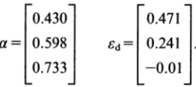
The remaining parameters of the model were chosen as follows. The interest rate - = 0.01 per quarter which reflects historical U.S. values. For lack of better information, equal bargaining power was assumed by setting /3=0.5. The elasticity of the matching function with respect to search input was set at 0 = 0.5 as well which is midway between the estimate obtained by Blanchard and Diamond (1989) using U.S. data and that of Pissarides (1986) from U.K. data. The scale parameter in the job matching function, k, and net average productivity, p - b, were set to approximate the mean, approximately 8.5%, and the vari- ability, 7% to 10%, of U.S. Manufacturing unemployment in the 1970s and 1980s. Finally, the job-specific component arrival rate, i%, and the dispersion parameter of the job-specific component, a, were set to match the average mean and standard deviation of job creation generated in the simulation with those reported for U.S. Manufacturing by Davis and Haltiwanger (1991). The actual values of the parameters assigned for the purpose of simulating the model are summarized in Table 1.

The equilibrium unemployed worker meeting rates and reservation shocks for each of the three aggregate states needed to compute the simulation are given by the follwing vectors:

0.430

0.471

a

0.598

0.241

.

(42)

0.733 -0.01

TABLE II

Simulation results: Means (std errors) of 100 Simulated 66 Quarters Samples

Simulation statistics Data

Mean (c) 5.23 (0.37) 5.2'

Std. Dev. (c) 0.91 (0.43) 0.9'

Std. Dev. (d) 1.37 (0.68) 1.6'

Corr (c, d) -0.10 (0.28) -0.36'

Corr (v, u) -0.26 (0.32)

' U.S. Manufacturing job flow series, 1972:2-1988:4, Davis and Haltiwanger (1991).

in equation (39) are presented in Table II. The reported statistics are means (with standard deviations in parenethesis) based on 100 simulated samples each 66 quarters in length. Sample statistics for U.S. Manufacturing data on job flows for the 66 quarters from 1972:2 to 1988:4 are included for comparison. In the table c and d represent rates of job creation and job destruction defined as the respective flows normalized by the average of employ- ment at the beginning and end of each period. Finally, u and v represent unemployment and vacancy rates respectively.

The results in Table II suggest the calibrated model can explain the co-movement and variability found in the Davis and Haltiwanger data on job creation and job destruction in U.S. Manufacturing. Specifically, for the parameter values that induce a match of the model's mean and standard deviation of job creation with the data, both the observed correlation between creation and destruction and the observed standard deviation of job destruction are within one standard error of the model's means. Although observing realized standard deviations of job creation and job destruction of roughly equal magni- tude is not unlikely due to the rather large sampling variation implied by the model, the average values implied by the model predict the observation that job destruction is more volatile over the available sample of 66 quarters. Finally, the model also implies a Beveridge curve as reflected in the negative correlation between unemployment and vacancies.

5. CONCLUSIONS

The model outlined in this paper is characterized by potentially large amounts of job creation and job destruction, due to idiosyncratic shocks that take place independently of the processes that change aggregate conditions. Changes in aggregate conditions, however, do affect the cutoffs that induce firms to open new jobs or close existing ones. So, if we interpret different phases of the cycle as equilibrium at different levels of the parameters (in our formulation, of different values taken by the common component of price, p, and the variance of the idiosyncratic shock, ao), job reallocation can vary over the cycle, even if the processes that cause it do not.

MORTENSEN & PISSARIDES JOB CREATION AND DESTRUCTION 413

are consistent with Davis and Haltiwanger's (1990, 1991) findings. Both results can be made stronger if aggregate events also change the degree of dispersion present in idiosyncratic shocks, provided the dispersion of productivities is lower at higher common component of labour productivity. At lower dispersion there is less job destruction, reinfor- cing the fall in job destruction due to higher common productivity, and less job creation, partially offsetting the higher job creation due to higher productivity. Our simulations, however, have shown that even holding dispersion constant, random changes in common price can proxy reasonable well the cyclical changes found in the U.S. data. In contrast, changes in the dispersion of productivities with constant aggregate productivity do not seem consistent with the finding that job creation and job destruction move in opposite directions during the cycle, so they are unlikely to be the domininant driving force of the unemployment cycle.

The aggregate unemployment model with endogenous job destruction behaves simi- larly to the standard model with exogeneous job exit, except that now shocks to the aggregate component of the value of product shift the Beveridge curve. Thus, if there are simultaneous aggregate and reallocation shocks, the Beveridge diagram ceases to be as useful a tool of analysis, because the two equilibrium curves in vacancy/unemployment space depend on a similar set of parameters. In these circumstances, the relation between job matchings on the one hand and job vacancies and unemployment on the other might shed more light on the source of shocks than might the relation between the stock of unemployment and the stock of vacancies. The information contained in vacancy/unem- ployment flow data is potentially more useful in distinguishing between different kinds of shocks than the information contained in the stocks.'0

APPENDIX Steady-state Ed and v/u: dependence on some parameters

The equilibrium conditions of interest are (10) and (13), drawn in Figure 1. In this Appendix we derive some of the results discussed in the text. For notational convenience let, in this Appendix, 0 stand for the ratio v/u and _-l for the elasticity of q(v/u). By the homogeneity of the matching function, 0 < q < _{1, though l is not} generally a constant.

Dependence on A

Differentiation of (10) with respect to A gives,

r +)LF( Sd) aSd P3C c9 0 a

r+)u a [1-l F(x)Jdx. (Al)

Differentiation also of (13) with respect to A gives,

q 90) 0= c __ r___ A)___ Ed__A.2 A _0fl

)CF(9u-+d) (-MC)(Eu-+d)2 DA2

Since q'(0)

<o0,

[q'(o)-

]00

(1-f)a[r+AF(9d)J 8u-d DA r+) r +)F(Ed) E Su ?d

The term in the square brackets of the left-hand side is negative and the term in the square brackets of the right- hand side is positive by virtue of the fact that

vEu

{ [1

-F(x)Jdx < Eu-? d, _(A4)

so 00/OA <0; job creation drops when job-specific shocks become less persistent.

Dependence on r

Differentiation of (10) with respect to r gives,

OSd flc(r+ A) _@0+ A Eu I-F(x) _dx. (A5) Or (I -fl)a[r +F(Ed)] Or r+ A r+F(Ed)

Differentiation of (13) gives,

00 c E

a(su-sd )q'(0) +, +aq()- (A6)

Therefore, 00/Or <0. To find the sign of Osd/Or, express first (A6) in elasticity form,

00- 0 + 0 Od (A7)

Or i1(r+A) ?1(Su -d) Or

and substitute subsequently into (A5):

+ flc(r +,A) 0 1 Od 1 3CO _{_+} f6a _I-Fxlx 1 ₍₈

[ _{(I-fl)c[r+AF(Ed)J11(Eu-Ed) or a[r+)AF(sd)J[ (1-,B)?1 r+A, [ (A8)}

The sign of the right-hand side of (A8) is generally ambiguous.

Dependence on a

Differentiation of (10) with respect to a gives,

r + F(Ed) OSEd PiC 00 e.

a+tltz9d) --6d= pC _{(38_6d-}

J

r +)u Da 1-f3Da r+)

Differentiation of (13) gives,

r(EU Ed) a00 = Eu SEd

d

* (A10)

00Da Da

Substitution of Osd/Oa from (A9) into (10) implies that 001/a has the sign of

4U + l[+ F(( )J

Ed +

1 _- F(x) _{dx1 =6u+ [ IF(s d)}

l E(6 I E >-d)> 0 (Al l) r

r+ F(Ed) Id lF(Ed) J r + AF(Ed) Esss) Al

The positive sign follows from the fact that E(?) = 0. Therefore 001/a > 0, regardless of the relation between p and b.

Substitution of 001/a from (AIO) into (A9) shows that the sign of OEd/00r is the same as the sign of the expression

- a6dd A [I-F(x)dx =p- b + 3 ( 1) (A12)

Therefore, p _ b is sufficient to ensure that when the effect of a on equilibrium v/u is taken into account, Ed is higher when a is higher.

MORTENSEN & PISSARIDES JOB CREATION AND DESTRUCTION 415 comments of Guiseppe Bertola, Hugo Hopenhayn, Richard Rogerson, Gerard van der Berg, John Shea and three anonymous referees.

REFERENCES

BERTOLA, G. and CABALLERO, R. J. (1991), "Efficiency and the Natural Rate of Unemployment: Labor Hoarding in Matching Models" (Unpublished, read at the NBER conference on Unemployment and Wage Determination).

BLANCHARD, 0. J. and DIAMOND, P. A. (1989), "The Beveridge Curve", Brookings Papers on Economic Activity, 1, 1-76.

BLANCHARD, 0. J. and DIAMOND, P. A. (1990), "The Cyclical Behavior of Gross Flows of Workers in the U.S.", Brookings Papers on Economic Activity, 2, 85-143.

BOERI, T. and CRAMER, U. (1991), "Why Are Establishments So Heterogeneous? An Analysis of Gross Job Reallocation in Germany" (Unpublished).

CABALLERO, R. J. and HAMMOUR, M. L. (1991), "The Cleaning Effect of Recessions" (mimeo). CONTINI, B. and REVELLI, R. (1988), "Job Creation and Labour Mobility: The Vacancy Chain Model and

Some Empirical Findings" (R & P Working Paper No. 8/RP, Torino).

CHRISTIANO, L. J. (1990), "Solving the Stochastic Growth Model by Linear-Quadratic Approximation and by Value Function Iteration", Journal of Business and Economic Statistics, 8, 23-26.

DAVIS, S. J. and HALTIWANGER, J. (1991), "Gross Job Creation, Gross Job Destruction and Employment Reallocation" (Unpublished).

DAVIS, S. J. and HALTIWANGER, J. (1990), "Gross Job Creation and Destruction: Microeconomic Evidence and Macroeconomic Implications" (Bureau of Census, CES Paper 90-10).

DIAMOND, P. A. (1982), "Wage Determination and Efficiency in Search Equilibrium", Review of Economic Studies, 49, 217-27.

JACKMAN, R. A., LAYARD, R. and PISSARIDES, C. A. (1989), "On Vacancies", O.xford Bulletin of Econom- ics and Statistics, 51, 377-394.

LEONARD, J. (1987), "In the Wrong Place at the Wrong Time: The Extent of Frictional and Structural Unemployment," in Kevin Lang and Jonathan Leonard (eds.) Unemployment and the Structure of Labor Markets (New York: Blackwell).

MORTENSEN, D. T. (1982), "The Matching Process as a Non-cooperative/Bargaining Game", in J. J. McCall (ed.), The Economics of Information and Uncertainty (Chicago: University of Chicago Press).

MORTENSEN, D. (1990), "Search Equilibrium and Real Business Cycles" (Unpublished, presented at the World Congress of the Econometric Society, Barcelona, August 1990).

MORTENSEN, D. (1993), "The Cyclical Behaviour of Job and Worker Flows" (mimeo).