Marta Mesquita, Margarida Moz, Ana Paias and Margarida Pato

A decomposition approach to the integrated

vehicle-crew-rostering problem

Marta Mesquita, Margarida Moz, Ana Paias and Margarida Pato

A decomposition approach to the integrated vehicle-crew-rostering problem

Marta Mesquita1,4, Margarida Moz2,4, Ana Paias3,4*, Margarida Pato2,4

1

Universidade Técnica de Lisboa, Instituto Superior de Agronomia, Dept. Matemática, Tapada da Ajuda, 1349-017 Lisboa, Portugal.

2

Universidade Técnica de Lisboa, Instituto Superior de Economia e Gestão, Dept. Matemática, Rua do Quelhas nº 6, 1200-781 Lisboa, Portugal.

3

Universidade de Lisboa, Faculdade de Ciências, DEIO, Bloco C6, piso 4, Cidade Universitária,1749-016 Lisboa, Portugal.

4

Centro de Investigação Operacional da FCUL

* Corresponding author: ampaias@fc.ul.pt

Abstract

The problem addressed in this paper is the integrated vehicle-crew-rostering problem (VCRP) aiming to define the schedules for the buses and the rosters for the drivers of a public transit company. The VCRP is described by a bi-objective mixed binary linear programming model with one objective function aggregating vehicle and crew scheduling costs and the other the rostering features. The VCRP is solved by a heuristic approach based on Benders decomposition where the master problem is partitioned into daily integrated vehicle-crew scheduling problems and the sub-problem is a rostering problem.

Computational experience with data from a bus company in Lisbon shows the ability of the decomposition approach for producing a variety of potentially efficient solutions for the VCRP within low computing times.

Keywords: integrated vehicle-crew-rostering problem, Benders decomposition, multi-objective optimization.

This paper focuses on the operational planning phase of a public transit company that operates buses in an urban area. The problem addressed aims to assign drivers of a company to vehicles and vehicles to a set of pre-defined timetabled trips that cover passenger transport demand on a specific area, during a planning horizon. The objective is to minimize total costs and maximize drivers’ preferences while satisfying passengers demand and driver constraints specified by general legislation, labor contracts and specific company rules. Due to the complexity of the corresponding combinatorial optimization problem, it is usually tackled on a sequential basis beginning with vehicle scheduling, followed by crew scheduling and, lastly, driver rostering. Given a set of timetabled trips, vehicle scheduling produces the set of daily schedules for the vehicles that perform all trips. The crew scheduling defines the daily crew duties that cover the respective vehicle schedules. Finally, for the planning horizon, crew duties are assigned to the company’s drivers leading to a roster that must comply with rostering constraints. There is a high dependency among these three problems, hence following this sequential approach one cannot guarantee that the final result is the best solution to the overall problem.

Despite its computational burden, the integration of all or some of these problems is expected to outperform the corresponding sequential approach. Efficient algorithms have been developed to solve the integrated vehicle-crew scheduling problem (Borndörfer et al. (2006), Huisman et al. (2005), Hollis et al. (2006), Mesquita and Paias (2008)). Crew-rostering integration has been devised by Caprara et al. (2001), Ernst et al. (2001), Freling et al. (2004) and Lee and Chen (2003) albeit within other transport contexts (railway and air crews) and by Chu (2007) for airport staff. In Mesquita et al. (2008) advantages of integrating the three problems for public transit companies were pointed out. For an overview of problems arising in the transport domain, see Barnhart and Laporte (2007).

represents the interests of the management, other objectives, like evenly distributing overtime among drivers and fulfilling as much as possible the preferences of drivers for specific crew duties, arise from the drivers priorities. These non-reconcilable interests at the operational planning phase suggest a multi-objective mathematical model for VCRP.

In this paper, the authors developed an integrated approach to solve the VCRP based on Benders decomposition. The method iterates between the solution of an integrated vehicle-crew scheduling problem and the solution of a rostering problem.

Benders decomposition methods have already been proposed although within airline planning by Cordeau et al. (2001) and Mercier et al. (2005) for the integrated aircraft routing and crew scheduling problem and by Mercier and Soumis (2006) for integrated aircraft routing, crew scheduling and the flight retiming problem. The solution approaches proposed by these authors are based on three phases. In phase 1, the linear programming relaxation of the problem is solved by Benders decomposition. Phase 2 considers all cuts generated during phase1 and applies Benders decomposition with the integer master problem. Phase 3 reintroduces integrality constraints in the sub-problem. Also in the same application context, Papadakos (2009) presented a Benders decomposition approach to deal with the integrated fleet assignment, aircraft routing and crew scheduling problem where both the sub-problem and the master problem are solved by column generation.

This paper is organized as follows. The VCRP is presented in the section 2, along with its mathematical formulation. Section 3 is devoted to Benders methodology and section 4 to the description of the new solution approach. Finally, section 5 shows computational results and section 6 presents some conclusions.

2. Mathematical formulation

location of another trip, those from a depot to the start location of a trip (pull-out trips) and those from an end location of a trip to a depot (pull-in trips). The set of timetabled trips and deadhead trips performed by a vehicle on day h∈His a vehicle block. Each vehicle block starts and ends at the same depot.

A task is the smallest amount of work to be assigned to the same vehicle and crew and it corresponds to a deadhead trip followed by a trip. A changeover is the walking movement of a driver between two timetabled trips in order to change the vehicle. Each end location of a trip is a potential relief point where a changeover may occur. A crew duty is a daily combination of tasks that respects labor law, union contracts and internal rules of the company. These rules depend on the particular situation under study and usually constrain the maximum and minimum spread (time elapsed between the beginning and end of a crew duty), the maximum working time without a break, the break duration, etc. The crew duties can start (end) at a depot or at an end location of a trip.

A line of work is the sequence of crew duties and days-off, one per day, assigned to a particular driver during the planning or rostering horizon. A line of work for a particular driver must satisfy a certain number of constraints that result from the above mentioned regulations, namely: the driver must rest a given minimum number of hours between consecutive duties; he must work at most a given working time per week, a given working time during the planning horizon and a given number of consecutive days; he must get at least a given number of days-off per week and a given number of Sundays off in the planning horizon, as well as specific weekdays off and weekends off. A roster is the set of lines of work for the drivers of the company that covers all the crew duties during the planning horizon.

To formulate the VCRP a mathematical model similar to the one proposed in Mesquita et al. (2008) is considered and the required notation follows:

H = planning horizon, partitioned into days

α= number of weeks in H h

N = set of timetabled trips for day h

N = _h

H h

N

∈ , set of all timetabled trips for H

n = |N|

h

I = set of deadhead trips corresponding to all pairs of compatible trips on day h h

c

I = subset of Ih where a changeover may occur

T = Ih

H h∈

, set of deadhead trips corresponding to all pairs of compatible trips for H D = set of depots

d

ν = number of vehicles in depot d (vehicles are identical in each depot)

h st

L = set of crew duties covering the deadhead trip from the end location of trip s to the start location of trip t and covering trip t, on day h

h t

DL = set of crew duties covering the deadhead trip from any depot to the start location of trip t and covering trip t, on day h

h s

LD = set of crew duties covering the deadhead trip from the end location of trip s to any depot, on day h

h

L1 = early crew duties on day h

h

L2 = late crew duties on day h h

L = L DL LDh_s N s h t N t h st I t

s,)∈ h ∈ h ∈ h (

, set of crew duties for day h, partitioned into L1h

andL2h h

O = day-off on day h, the (|_Lh|+1)th "crewduty" M = set of drivers

u = spread of crew duty

'

u = max {0, u -u }, overtime of crew duty

b1w= maximum total work per week per driver

b

rw= maximum total work during H per driver

g = maximum number of consecutive days without a day-off for a driver

Ω

w= minimum number of days-off per week per driver

Ω

S= minimum number of Sundays-off during H per driver

= mh

e 1 if driver m was assigned to a crew duty on day h from the previous planning horizon, or 0 otherwise

m

F = set of obligatory days-off (planned absences, for instance) for driver m during H dh

st

c1 = cost of the deadhead trip from trip s to trip t plus trip t cost, performed by a vehicle from depot d on day h

h s d n h

d n

s c

c 1 , 1

, + , + = pull-in and pull-out costs from trip s to depot d and from depot d to trip s, respectively, on day h

2

c = cost of crew duty

c3m = cost of assigning work to driver m during H

c4= penalty cost for the maximum overtime per driver during H

mh

c5 = penalty cost based on driver m preference for crew duty on day h.

All the costs are assumed to be nonnegative. Now the decision variables are presented:

=

dh st

z 1 if a vehicle from depot d performs trips s and t in sequence on day h, or 0 otherwise

= +

h d n s

z _, 1 if a vehicle returns to depot d after trip s on day h, or 0 otherwise

= +

h t d n

z _, 1 if depot d directly supplies a vehicle for trip t on day h, or 0 otherwise

=

h

w 1 if crew duty is selected on day h, or 0 otherwise

=

mh

y 1 if driver m performs crew duty on day h, or 0 otherwise

=

ωm _{1 if driver m works during H, or 0 otherwise}

Then, the VCRP becomes the following bi-objective mixed integer linear programming problem: ∑ _       ∑ ∑ + ∑      ₊ + ∑ ∑

∈H ∈ ∈ ∈ ∈ + + + + _∈

h d Ds N _L

h h s d n h s d n h d n s h d n s D

d st T

dh st dh st h w c z c z c z

c 1_{, ,} 1 _{, ,} 2

) , ( 1 min (2.1)         ∑ ∑ ∑ + + ∑ ∈ ∈ _∈

∈ m Mh H L

mh mh M m m m h y c c

c3 4 5

min ω δ (2.2)

subject to

( ), , 1

:

=

+

∑

∑ ∑

∈ +

∈ ∈ d D

h t d n D

d s st I dh

st z

z

h

∀t∈Nh,∀h∈H (2.3)

( ), , :( ), , 0

: = − ∑ − + ∑ ₊ ∈ + ∈ h d n t I s t s dh ts h t d n I t s s dh

st z z z

z

h

h t N d D

h _{∀ ∈}

∈

∀ , ,∀h∈H (2.4)

d N s h s , d n h

z ≤

ν

∑

∈ +

∀d∈D,∀h∈H (2.5)

0

, =

∑ − ∑

∈DL d∈D +

h t d n h h t z

w ∀t∈Nh,∀h∈H (2.6)

0 =

∑ − ∑

∈L d∈D

dh st h h st z

w ∀

( )

s,t ∈Ih\I_ch,∀h∈H (2.7)

0 ≥

∑ − ∑

∈L d∈D

dh st h h st z

w ∀

( )

s,t ∈I_ch,∀h∈H (2.7)’

0 , = ∑ − ∑ ∈ +

∈ d D

h d n s LD h _z w h s h N s∈

∀ ,∀h∈H (2.8)

0 = −

∑

∈ w y h M m

mh _{∀ ∈L}h_{,∀h∈H (2.9)}

1 } { = ∑ ∪ ∈_Lh _oh

mh

y ∀m∈M,∀h∈H (2.10)

1 ) 1 ( _≤ ∑ + ∑ ∈ − ∈ ih _Ljh

h m L

mh _y

w l l h mh L b y u h 1 7 1 ) 1 ( 7 ≤ ∑ ∑ + − =

∈ ∀m∈M,l =1,...,

α

(2.12)

rw H h mh L b y u h ≤ ∑ ∑ ∈ ∈ M m∈

∀ (2.13)

g y h L g r r h m _≤ ∑ ∑ ∈ = + 0

, _{∀m∈M,h=1,...,|H|−g (2.14)}

g y

e h g

r mr L h r mr

h ∑ ≤

∑ + ∑ + = ∈ = 1 0

∀m∈M,h =1−g,...,−1,0 (2.14)’

Ω ≥ ∑ + − = w l l h mh y _h 7 1 ) 1 ( 7 ο

∀m∈M,l =1,...,α (2.15)

Ω ≥ ∑ = S l l m o l y α 1 7 ,

7 ∀m∈M (2.16)

0 ≤ − ∑ ∑ ∈ ∈ m L h H

mh _H y

h ω ∀m∈M (2.17)

0

' − ≤

∑ ∑

∈_Lh _h∈_H δ

mh y

u ∀m∈M (2.18)

{ }

0,1

∈

dh st

z ∀

( )

s,t ∈Ih,∀d∈D,∀h∈H (2.19)

{ }

01

, z ,

z_sh_{,n+d n}h_+d,s∈ ∀s∈Nh,∀d∈D,∀h∈H (2.20)

{ }

0,1 ∈

h

w ∀ ∈_Lh,∀h∈H (2.21)

{ }

0,1

∈

mh

y m M Lh h h H

O ∀ ∈

∪ ∈ ∀ ∈

∀ , { }, (2.22)

{ }

0,1

∈

m

ω

∀m∈M (2.23)

0 ≥

δ . (2.24)

The objectives of the VCRP derive from minimization of vehicle and driver costs, as

well as minimization of inconvenience of work for the drivers. In fact, on the one hand,

h d n s

c1_{, +} and c_n1h_+d,t. Besides, management often wants to know the minimum workforce

required to operate the fleet of vehicles, so as to assign drivers to other departments of the

company or to replace those absent. Such policy results in minimizing crew duty costs c2

associated to variables wh and rostering costs c3m associated to ωm, variables

representing drivers effectively assigned to work. On the other hand, interests of drivers

must be taken into account and this motivates the definition of penalty costs c4

associated with the overtime, since overtime is undesirable it should be minimized and

equitably distributed. Also penalty costs c5mh related to drivers’ preferences for specific

duties can be considered in the model. All these objectives represent various conflicting

interests that cannot usually be simultaneously fulfilled thus leading to a multi-objective

perspective for VCRP. However, more than two objectives are not easily tackled. Hence,

we opted by a bi-objective optimization problem: the first objective, (2.1), aggregates

vehicle and crew duty costs; the second objective, (2.2), aggregates driver costs plus

driver penalties, the rostering objective.

In the above bi-objective model, constraints (2.3)-(2.5) describe the vehicle scheduling

problem. Constraints (2.3) state that each timetabled trip is performed, exactly once, by a

vehicle that comes directly from a depot or from the end location of another timetabled

trip. Constraints (2.4) together with (2.3) ensure that, for each day, each timetabled trip is

performed, exactly once, by a vehicle that returns to the source depot, being constraints

(2.5) depot capacity constraints. Note that, for each day h∈H ,

{

( ) ( ) ( )

2.3, 2.4, 2.5

}

defines

an integer multi-commodity network flow problem.

The constraint set {(2.6), (2.7), (2.7)’, (2.8)} links vehicle and crew duty variables

ensuring that each task in a vehicle block is covered by one crew. (2.6) and (2.8) impose

the covering of tasks involving deadhead trips from/to depots and (2.7) and (2.7)’ refer to

covering the remaining tasks. Set Ih is partitioned into two subsets, I_chandIh \Ich.

Deadhead trips where changeovers may occur are included in I_ch. Constraints (2.7)

assign a single crew to each deadhead trip in Ih \Ich whereas constraints (2.7)’

correspond to two different situations. On the one hand, constraints (2.7)’ allow drivers to

location of the first trip is the same as the start location of the second one, this movement

represents a waiting time. On the other hand, they allow deadhead trips to be covered by

more than one crew. As over-covering only occurs if assigning several drivers to a task is

cheaper than assigning a single one, the major role of (2.7)’ is to explicitly handle

changeovers in the constraint set.

Constraints (2.9)-(2.16) define an assignment problem with additional constraints.

Equalities (2.9) link crew and rostering variables by imposing that each crew duty, in a

solution, must be assigned to one and only one driver and equalities(2.10) deal with the

assignment of each driver to one crew duty or to a day-off on each day. Constraints (2.11)

forbid the sequence of late/early duty followed by early/late duty to ensure that drivers

rest a given minimum number of hours between consecutive duties (a hard constraint

coming from legislation) and also that changes of shift are only allowed after a day-off (a

soft rostering constraint here imposed as if it was a hard one). Inequalities (2.12) and

(2.13) force drivers to work at most a given time per week and a given time during H.

Inequalities (2.14) and (2.14)’ impose for each driver the maximum number of days – g –

without a day-off. As to (2.14)’ they are defined for the first g days of H, taking into account the parameters for the crew duties assigned in the last days of the previous

planning horizon. Furthermore, (2.15) and (2.16) ensure for each driver at least a given

number of days-off per week and at least a given number of Sundays off in H,

respectively.

Constraints (2.17) define the variables

ω

m from the rostering variables ymh and

inequalities (2.18) calculate the maximum overtime per driver so as to minimize and

equitably distribute it through the second optimization objective.

Finally, (2.19)-(2.24) define the domains of the variables: a nonnegative space for δ

and binary sets for the remaining.

3. Decomposition Approach

The VCRP has been modeled as a huge dimension mixed binary linear optimization

problem that includes three main combinatorial structures: an integer multi-commodity

network flow problem (Mesquita and Paias 2008), a set partitioning/covering structure

Within those combinatorial structures two well known scheduling problems can be

identified: one defining the vehicle-crew scheduling process and the other the rostering.

These two sub-problems share a set of variables and (complicating) constraints, in spite

of involving other separable sets of variables and constraints. By taking into account the

variables involved in the complicating constraints, a Benders decomposition based

method arises as a natural approach to solve the overall problem, the VCRP. Such a

technique has been applied in different combinatorial optimization contexts as referred to

in the survey by Boschetti and Maniezzo (2009).

3.1 Benders decomposition

In 1962, Benders proposed a decomposition algorithm, for solving large single

objective mixed integer linear programming problems, that alternates between a primal

sub-problem and a master problem. The Benders sub-problem is a restriction of the

original problem where some decision variables’ values are fixed. In each iteration of the

algorithm the solution of the master problem is used to adjust primal variables’ values

that will be fixed in the sub-problem, whereas the dual sub-problem solution is used to

construct cuts - Benders cuts - to be added to the master. This method guarantees the

convergence to the optimum under specific hypotheses latter generalized (Geoffrion

1972).

The VCRP is indeed a very complex and huge dimension multi-objective

combinatorial problem that will be optimized from a Pareto perspective (Ehrgott and

Gandibleux 2000). As it is not reasonable to search for the entire Pareto frontier due to

such a demanding process on computing resources, the VCRP will be tackled within a

single objective issue by weighting the two original objective functions, that is, by

substituting (2.1) and (2.2) by:

+ ∑ _       ∑ ∑ + ∑      ₊ + ∑ ∑

∈H ∈ ∈ ∈ ∈ + + + + ∈

h d Ds N _L

h h s d n h s d n h d n s h d n s D

d st T

dh st dh st

hc w z

c z

c z

c 1_{, ,} 1 _{, ,} 2

) , ( 1 1 minλ         + ∑ _       ∑ ∑ + +

∈ ω ∈ _∈ δ

λ c c y c

M

m h H L

mh mh m m h 4 5 3 2

+ ∑ _       ∑ ∑ + ∑      ₊ + ∑ ∑

∈H ∈ ∈ ∈ ∈ + + + + _∈

h d Ds N L

h h s d n h s d n h d n s h d n s D

d st T

dh st dh st

h c w z

c z

c z

c λ λ λ

λ 1 1, , 1 1 , , 1 2

) , ( 1 1 min δ λ λ ω

λ c c y c

M

m h H _L

mh mh m m h 2 4 5 2 3 2 + ∑ _       ∑ ∑ + +

∈ ∈ _∈ (3.1)

where _λ1 and λ2 are nonnegative real parameters.

The non-supported efficient solutions of the bi-objective problem (2.1) to (2.24)

cannot be obtained from minimization of (3.1) subject to constraints (2.3) to (2.24) even

by taking into account all the possible choices for the weights _λ1,_λ2 (Steuer 1986).

However, a partial Pareto optimization strategy, not requiring the entire set of efficient

solutions, copes with the typical decision makers’ demand for a set containing a few

solutions, achieving different levels of quality for the objectives.

The mathematical model presented includes different types of decision variables.

Variables z define the vehicle schedules, variables w are associated to crew duties and variables y,

ω

and δ are connected with rostering. These variables may be partitioned

into two sets: the zw-set and the yωδ -set. The decomposition approach proposed, based

on Benders method, alternates between the solution of a master problem involving the

zw-set, a vehicle-crew scheduling problem for all the days of H, and the solution of the

corresponding sub-problem involving the yωδ -set, a rostering problem.

In order to present the sub-problem and the master problem, the VCRP defined by

(2.3) to (2.24) and (3.1) is supposed to possess a non-empty feasible region. Now, it is

rewritten through the following matrix form:

min λ₁

_c

1Z +λ₁

_c

2W+λ₂

_c

3

ω

+λ₂C4δ +λ₂

_c

5Y (3.2)

subject to

2 1_{Z A}

A ≥ (3.3)

3 2 1 B W B Z

B + ≥ (3.4)

0

= −W QY (3.5) E Y

E1 ≥ 2 (3.6)

3 2

1_{Y G G}

G +

ω

≥ (3.7)

0

1

≥ +δ

0

≥

Z and binary (3.9)

0

≥

W and binary (3.10)

0

≥

Y and binary (3.11)

0

≥

ω

and binary (3.12)

0 ≥

δ (3.13)

where

_c

1,

_c

2,

_c

3,

_c

5, A1, A2, B1, B2, B3,Q, E1, E2,G1, G2, G3,P,

1

,

0

,Z,W,Y _and

ω

are appropriate dimension matrices.

Here (3.2) stands for (3.1), (3.3) corresponds to (2.3)-(2.5), (3.4) represents

(2.6)-(2.8), (3.5) corresponds to (2.9), (3.6) stands for (2.10)-(2.16), (3.7) for (2.17), (3.8)

represents inequalities (2.18), and, finally (3.9)-(3.13) correspond to (2.19)-(2.24).

3.2. Sub-problem

Fixing the values of the z and w variables in VCRP at values given by vectors Z and

W , respectively, the following sub-problem is obtained:

(

Subzw

)

min λ2

c

3

ω

+λ2c4δ +λ2

c

5Y +

(

λ1

c

1Z+λ1

c

2W

)

(3.2)’

subject to

W

QY = (3.5)’

E Y

E1 ≥ 2 (3.6)

3 2

1_{Y G G}

G +

ω

≥ (3.7)

0

1

≥ +δ

PY (3.8)

0

≥

Y and binary (3.11)

0

≥

ω

and binary (3.12)

0

≥

δ

. (3.13)

As one considers the set of crew duties and vehicle blocks induced by (Z ,W ), this

sub-problem is a rostering problem. Moreover, if (Y,

ω

,δ ) is a feasible solution for

w z

Sub and (Z ,W ) satisfies (3.3), (3.4), (3.9) and (3.10) then

(

Z,W,Y,

ω

,δ

)

is feasible

Let us denote by LSubzw the linear programming relaxation of Subzw, where (3,11),

(3.12) are replaced by Y≥

0

and

ω

≥

0

, respectively. A new set of constraints, (3.14), is

added to set unitary bounds on the

ω

variables:

1

≤

ω

I

(3.14)

where

1

is an appropriate dimension unitary vector and I an identity matrix. Note that, unitary bounds for the y variables are not necessary since constraints (2.10) and (2.11), included in matrix representation (3.6), force these variables to be less than or equal to 1.

Let

ς

,

β

,

φ

,χ and

ε

be the dual vectors corresponding to (3.5)’, (3.6), (3.7), (3.8)

and (3.14), respectively. Then, the dual of the linear programming problem LSub , zw

denoted by DLSubzw, can be written as:

(

DLSubzw

)

max

ς

W +βE2+

φ

G3+

ε

1+

(

λ1

c

1Z +λ1

c

2W

)

(3.15)

subject to

c

I

G2

ε

λ2 3

φ

+ ≤ (3.16)

c I λ₂ 4

χ ≤ (3.17)

c

P G E

Q β 1

φ

1 χ λ2 5

ς

+ + + ≤ (3.18)

0

,

0

,

,

φ

χ

≥

ε

≤

β

. (3.19)

If the drivers, defined by set M, with the respective availabilities from mh

e and m

F ,

are enough to cover all crew duties for all days of H, given by W and at the same time all

the rostering constraints are satisfied, assuming all variables may be non-integer, then

w z

LSub has feasible solution and optimal solution also (note that the respective feasible

regions are bounded along the optimization direction). In this case, a Benders cut is

obtained from the optimal solution of DLSub_zw which corresponds to an extreme point

of the respective feasible region. If the available drivers are not enough to cover all the

crew duties in W respecting all rostering constraints even accepting fractional variables,

then LSub is unfeasible and its dual, zw DLSubzw, is unbounded (there is always at least a

feasible dual solution, the nil vector). In this case the corresponding Benders cut is

3.3. Master problem

Let PD and RD be, respectively, the set of the extreme points and the set of extreme

rays of the dual feasible region defined by (3.16) to (3.19), according to the Benders

decomposition theory the master problem follows:

(Master)

min ϕ₀ (3.20)

subject to

1

3 2

2 1 1

1

0 λ (

ς

λ ) β

φ

ε

ϕ ≥

_c

Z+ +

_c

W + E + G + (

ς

,β,

φ

,χ,

ε

)∈PD (3.21)

1

3 2

0≥µW +η E + G + (µ,η, , )∈RD (3.22)

A Z

A1 ≥ 2 (3.3)

3 2 1_{Z B W B}

B + ≥ (3.4)

0

≥

Z and binary (3.9)

0

≥

W and binary. (3.10)

The constraint set {(3.3), (3.4), (3.9), (3.10)} is also included in the mathematical

model of the VCRP where it describes the integrated vehicle-crew scheduling problem

for all the days of the planning horizon. This fact suggested the decomposition procedure

for the VCRP that will be detailed in the next section.

4. Solution approach

Let VCRP_y,ω≥0 be the problem obtained from relaxing the integrality constraints for

the y and

ω

variables in VCRP defined through (3.2) to (3.13) with a specific choice for

the parameters_λ1and_λ2. Fixing the values of the z and w variables in VCRP_y,ω≥0 at

values given by vectors Z and W , respectively, we obtain the linear sub-problemLSub_zw

and Benders decomposition theory guarantees that an optimal solution for VCRPy,ω≥0 is

achieved, in case it exists (see Benders 1962). However, such optimal solution might not

be feasible for VCRP due to the possibility of obtaining non-integer values for the y and

ω

variables. In fact, the sub-problem Sub_zwis a mixed binary linear programming

forced to be binary) and for this case, to the authors’ knowledge, no Benders convergence

results have been generalized.

For each specific choice of values for parameters_λ1and _λ2, this paper proposes a

non-exact approach for VCRP that iterates between a vehicle-crew scheduling problem

for the planning horizon and a rostering problem thus obtaining, at the end, a feasible

solution for the VCRP that naturally might not be an optimal one. In addition, this

decomposition method is also much useful insofar as, along the several iterations, it

produces a pool of feasible solutions for the VCRP. Such solutions can be analyzed from

the two original objectives’ perspective and one can determine the potentially efficient

solutions corresponding to the points of the objectives’ space that are not dominated by

other points in the pool, the so-called potentially non-dominated points.

The Decomposition algorithm is summarized in figure 1.

Decomposition algorithm //input//

Data: λ₁,λ₁,

c

1,

c

2,

c

3,c4,

c

5, A1, A2, B1, B2, B3,Q, E1, E2,G1, G2, G3,P

//initialization//

step1) PD0 = RD0=Pool=Φ.

step 2) k=1. //iteration k//

step 3) Define Masterk with the cuts from PDk-1and RD k-1.

step 4) Define RMasterk

( )

U,V , a lagrangean relaxation of the cuts associated to multipliers U and

V satisfying 1 1

1

=

∑

=

k

i i u .

step 5) Solve RMasterk

( )

U,V .

5.1) Apply the integrated vehicle-crew scheduling algorithm for each day of H.

5.2) Concatenate the |H| solutions thus building a feasible solution of the vehicle-crew scheduling

problem for H,

( )

Z,W .

step 6) Call procedure Sub-problem(k;

( )

Z,W ;PD k-1;RD k-1;Pool).

//stoping criterion//

step 7) If k≤maxiterations−1

7.2) otherwise, calculate the potentially efficient solutions from the Pool. Stop.

Figure 1. Decomposition algorithm for the VCRP.

Steps 3, 4 and 5 of each iteration of the Decomposition algorithm are devoted to the

master problem whereas step 6 calls the procedure to tackle the sub-problem. These

features will be detailed in the next sub-sections.

4.1. Solving the master problem

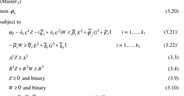
Suppose that, in iteration k, PD_k has k1 extreme points and RD_k has k2 extreme rays.

Then the master problem becomes:

(Master k)

min

ϕ

0 (3.20)

subject to

1

3 2

2 1 1

1

0 λ (

ς

λ ) β

φ

ε

ϕ −

_c

Z− _i+

_c

W≥ _iE + _iG + _i i = 1,…, k1 (3.21)’

1

3 2

i i

i

iW ≥ E + G +

−

µ

η

i = 1,…, k2 (3.22)’

A Z

A1 ≥ 2 (3.3)

3 2 1_{Z B W B}

B + ≥ (3.4)

0

≥

Z and binary (3.9)

0

≥

W and binary (3.10)

where _{i i k}

i i

i, , , , )∈PD

(

ς

β

φ

χ

ε

and (

µ

_i,

η

_i, _i, _i)∈_RDk.

The master problem is a difficult binary linear programming problem and must be

solved repeatedly, i.e., in each iteration of the algorithm. Moreover, the convergence

results of the Benders algorithm to an optimal solution do not apply here, as mentioned

above, due to the combinatorial nature of the sub-problem,Subzw. Consequently, a

non-exact approach to tackle the master problem is advisable. The option favoured a method

Masterk is considered, where (3.21)’ and (3.22)’ are embedded in the objective function

associated with the non-negative lagrangean multipliers U and V, respectively:

(

)

(

RMaster_k U,V

)

min + ∑

= 1 1 0 k i i u

ϕ

(

−ϕ0+λ1

c

1Z+(

ς

i +λ1

c

2)W +ri

)

+∑

=

2

1

k

i i

v

(

µ_iW +s_i

)

(4.1)

subject to

A Z

A1 ≥ 2 (3.3)

3 2 1_{Z B W B}

B + ≥ (3.4)

0

≥

Z and binary (3.9)

0

≥

W and binary (3.10)

where 2 3

1

i i

i

i E G

r =

β

+

φ

+

ε

for all i=1,...,k₁ and 2 3

1

i i

i

i E G

s =

η

+ + for all

2

,..., 1 k i = .

Note that, the integrality property is not valid for RMasterk

(

U,V

)

. As a result, in each

iteration k, one has v

(

_k

)

_k

(

U V

) (

v _k

)

V

U RMaster , Master

LMaster

0 ,

max ≤

≤

≥ , where v(LMasterk)

is the optimal value of the linear programming relaxation of Masterk. Hence, the

lagrangean relaxation might do better than the linear relaxation in what respects lower

bounds for v(Masterk). Usually, the values of the lagrangean multipliers associated to the

relaxed constraints are set equal to the values of the corresponding dual variables and an

optimizing iterative procedure updates the multipliers so that the lower bound improves.

However, in this approach no multiplier improvement is performed.

A specific choice for the lagrangean multipliers values, U and V , such that

1 1 1 = ∑ = k i i

u (satisfied by the corresponding dual variables), converts the objective function of

( )

U V k ,

RMaster , in (4.1), into:

∑ + = 1 1 0 k

i ui

ϕ

(

−ϕ0+λ1

c

1Z +(

ς

i +λ1

c

2)W +ri

)

+∑

=

2

1

k

i vi

(

i i

)

s W +

µ =

=

c

Z _u i

c

W

k

i i 

    + ∑ + = 2 1 1 1 1 1 λ

λ

ς

i

k i i r u ∑ + = 1 1 + ∑ = 2 1 k i i

v µ_iW k _i i i s v ∑ + = 2 1 =

= Z _u i k _{vi i} W

k i

c

c

      ∑ + + ∑ + =

= λ

µ

λ

ς

2 2

Now, this objective function can be rewritten by identifying the components of the

vectors

_c

1,Z,

_c

2andW :

(

)

+ ∑       ∑ ∑ + + ∑ + ∑ ∑

∈H ∈ ∈ ∈ ∈ + + + + ∈

h d Ds N L

h h s d n h s d n h d n s h d n s D

d st T

dh st dh st h w c z c z c z c 2 , 1 , 1 , 1 , 1 ) , ( 1

1 λ λ

λ + i k i i r u ∑ = 1 1 i k i i s v ∑ + = 2 1

where k _i

i i i

k

i ui c v c = ∑

ς

+λ + ∑

µ

= = 2 1 2 1 1

2 1 _.

For any choice for the parameter_λ1, since k _i

i i r u ∑ = 1 1 i k i i s v ∑ + = 2 1

is constant, this objective

function, along with the set of constraints of RMaster_k

( )

U,V , can be partitioned into |H|

independent subsets. Therefore, solving RMasterk

( )

U,V for a specific choice of the

multipliers Uand V is equivalent to solving |H| independent integrated vehicle-crew

scheduling problems, one for each day of the planning horizon. The (daily) integrated

vehicle-crew scheduling problems can be solved by the algorithm proposed in Mesquita

and Paias (2008) which combines a heuristic column generation procedure with a

branch-and-bound scheme.

Note that these vehicle-crew scheduling solutions may give slightly different daily

schedules for the vehicles and also for the crews. However, in real cases public transit

companies, usually, have the same vehicle-crew schedules in each day type of the

planning horizon - there is a pattern for the weekdays and one pattern for the weekend

days. Hence, it is desirable that solutions resulting from the master problem will follow

this scheme. Consequently, in step 5 of the Decomposition algorithm the master problem

is solved for each day type.

4.2. Solving the sub-problem

In each iteration of the Decomposition algorithm, step 6 (figure 1) refers to the

sub-problem. Figure 2 details the procedure.

Procedure Sub-problem(k;

( )

Z,W ;PD k-1;RD k-1;Pool)

step 1) Define Sub_zw, the rostering sub-problem for iteration k

step 2) Solve LSub_zw, the corresponding linear relaxation:

2.1) in case it has a finite optimal value, save the corresponding dual solution and go to step 3; 2.2) in case it is unfeasible, save an extreme ray of the dual linear feasible region and go to step 5.

step 3) Solve Sub_zwto get a feasible roster if the threshold π is not attained. //solutions for the VCRP//

step 4) Update the Pool of feasible solutions of the VCRP.

step 5) Update the sets of extreme points and of extreme rays, PD k-1 and RD k-1.

Stop.

Figure 2. Procedure for tackling the sub-problem.

Exact standard algorithms are used to solve the sub-problem (step 3) and the

respective linear relaxation (step 2), Subzw and LSubzw. The dual linear variables or dual

extreme rays obtained in step 2 will give rise to the Benders cuts that will be added to the

master problem, in the next iteration.

Let v

(

LSubzw,k−1

)

denote the linear programming relaxation value in iteration k-1 of

the Decomposition algorithm. To obtain a feasible roster, a branch-and-bound is executed

with Subzw whenever the following criterion involving the two optimization objectives

and a threshold π (step 3) is satisfied:

(

_{zw k}

)

≤

vLSub ,

1 ,..., 1min−

= k

i v

(

LSubzw i

)

+

π

or

v

(

RMasterk

(

U V,

)

)

≤

1 ,..., 1min−

= k

i v

(

RMasteri

(

U V,

)

)

+π.

In this case, the solution of the master, a set of vehicle-crew schedules covering the

planning horizon, along with the solution of the sub-problem correspond to a feasible

solution for the VRCP which will be included in the Pool - step 4 of the procedure in figure 2.

5. Computational experiment

A computational experiment was performed using real-world data from a public

All linear programming relaxations and branch-and-bound schemes, in the

Decomposition algorithm, were tackled with CPLEX solvers (CPLEX Manual version

11.0, 2007). As for the integer resolution of the rostering sub-problems a time limit of

7200 seconds was imposed. The (daily) integrated vehicle-crew scheduling problems

were solved by the algorithm proposed in Mesquita and Paias (2008) by setting the

parameters

∈

=7,

γ

=3000 and p=4/15, where

∈

is the parameter related with the definition

of the tasks,

γ

is the maximum number of columns generated per iteration and p is a parameter related with the heuristic pricing of the columns. See Mesquita et al. 2009 for a

detailed description of these parameters.

All algorithms were coded in C, using VStudio 6.0/C++ and all the programs ran on a

PC Pentium IV 3.2 GHz.

5.1 Test instances

The test instances used for the experiments were derived from an urban bus service

inside the city of Lisbon and involve scheduling problems with 122, 168, 224, 226 and

238 trips and 4 depots. The input of each VCRP instance includes the start and end times,

the start and end locations for each trip and the deadhead times between locations and

depots. Two different demand patterns (timetabled trips) are considered, one for

weekdays and the other for weekend days. Consequently, in each iteration of the

Decomposition algorithm the integrated vehicle-crew scheduling problem is solved

twice: for a weekday type and for a weekend day type.

Concerning daily crew duties and the rostering, some parameters have to be defined

in order to respect the rules imposed by Portuguese Law, union contracts and specific

rules of the bus company. A detailed description of them may be seen in Mesquita et al.

(2008).

In what respects the vehicle-crew scheduling process one has:

- for each crew duty the minimum spread is set at 1 hour

- the maximum spread is 5 hours for duties without a break; otherwise, it is 10 hours and

45 minutes

- break times range from 1 hour to 2 hours and 20 minutes

- a penalty of 5000 m.u. is added to the cost of each pull-in and each pull-out trip in order

to minimize the number of vehicle blocks in the schedule

- _λ1=1.

Respecting the rostering process one has:

- |H|=28 - α =4

- |M|=80

- u ∈

[

300 ,645

]

minutes

- u = 480 minutes (8 hours)

- a = 11 hours - the minimum rest period of 11 hours allows the separation of the set of

crew duties into early duties (_L1h_{), starting at a point between 6:00 a.m. and 3:30 p.m. and}

late duties (L2h), starting in the interval from3:30 p.m. to midnight

- b1w = 2880 minutes (48 hours)

-

_b

_rw = 10560 minutes (176 hours)

- _Ωw = 2 days

- ΩS = 1 day

- g = 6 days

- Fm = ∅

- c3m = 0.96

- c4= 0.04

- c5mh = 0

- λ2=1

- π = 0.

5.2 Computational results for the VCRP

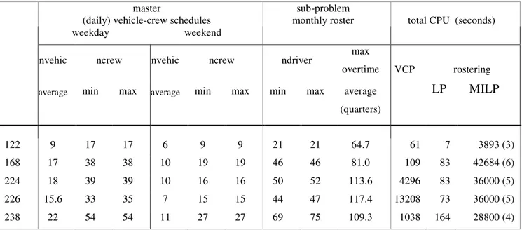
Tables 1 and 2 show computational results obtained from 10 iterations of the

proposed Decomposition algorithm. In both tables, “nvehic”, “ncrew” and “ndriver” refer

table 1, column (10) contains the average maximum overtime per driver measured in

units of 15 minutes. The last columns in table 1 are devoted to CPU time: the values

reported in columns (11) and (12) are total CPU values obtained from the 10 iterations,

respectively, for the VCP master problem and for the linear programming relaxation

rostering sub-problem. Column (13) shows total CPU values for determining

mixed-integer solutions of the rostering sub-problems (feasible rosters) and, in brackets, the

number of MILP sub-problems solved according to the threshold π.

Table 1. Results from 10 iterations of the Decomposition algorithm.

As one can see, in table 1, the Decomposition algorithm has produced solutions that,

despite being different, have the same number of vehicles and crews. Variations have

occurred only for instance 226. This diversity of vehicle-crew solutions led to rostering

solutions that, for the same instance, may have a great variation in the number of drivers.

For instance 224 the rostering solutions differ at most in 2 drivers. For the last two

instances, 226 and 238, the number of drivers varies from 44 to 47 and 69 to 75,

respectively.

On average, considering all instances, the rostering mixed integer linear program

(MILP) was solved 5 times out of 10. One can notice that, for each instance, a small

master sub-problem

(daily) vehicle-crew schedules monthly roster total CPU (seconds)

weekday weekend

nvehic ncrew nvehic ncrew ndriver max

overtime VCP rostering

average min max average min max min max average (quarters)

LP MILP

122 9 17 17 6 9 9 21 21 64.7 61 7 3893 (3)

increase in the number of mixed integer linear rostering problems solved, during 10

iterations, led to a great increase in total CPU time.

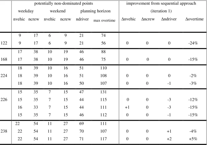
In table 2, for each instance, the first row of columns (2) to (7) shows the results

obtained in the first iteration of the Decomposition algorithm which corresponds to that

of a sequential approach applied to the same instance. The subsequent rows (or row), in

columns (2) to (7), correspond to the potentially non-dominated points (or point)

obtained. Columns (9) to (11) report on the difference between the solution

corresponding to a potentially non-dominated point - potentially efficient solution - and

the solution obtained on iteration 1 (sequential approach), concerning the number of

vehicles, the number of crew duties, the number of drivers and the overtime. The last

column refers to overtime and is given in percentage.

Table 2. The Decomposition algorithm versus the Sequential algorithm.

potentially non-dominated points improvement from sequential approach weekday weekend planning horizon (iteration 1)

nvehic ncrew nvehic ncrew ndriver _{max overtime} ∆nvehic ∆ncrew ∆ndriver ∆overtime

122 9 9 17 17 6 6 9 9 21 21 74

56 0 0 0 -24%

168 17 17 38 38 10 10 19 19 46 46 88

75 0 0 0 -15%

With the exception of instance 238, the potentially non-dominated points obtained by

the Decomposition algorithm dominate the points obtained by the sequential approach

(see the first row - first iteration - per instance). In instance 238, the first solution

obtained by the Decomposition algorithm, is itself a potentially efficient solution. The

last row of the table displays a point for this instance that corresponds to a reduction in

the cost of the weekday VCP thus being a potentially non-dominated point.

In general, one can see from the above results that the improvement over the first

solution is obtained by minimizing the maximum overtime per driver. In fact, the solution

of the master problem could be adjusted using the feedback obtained by introducing

Bender cuts. This feedback guided the building of the vehicle and crew schedules thus

conducing to rosters with less overtime per driver and with fewer drivers. Note that,

although a sequential approach greatly reduces CPU time, the resulting integrated

problem might not be solvable if no feasible roster can be built from the vehicle-crew

scheduling solution.

6. Conclusions

This paper proposes a new methodology to deal with the integrated

vehicle-crew-rostering problem within public transit companies. The VCRP is modelled as a

bi-objective mixed binary linear problem and the solution approach is based on Benders

decomposition. It alternates between the solution of an integrated vehicle-crew

scheduling master problem and the solution of the corresponding linear programming

relaxation rostering sub-problem, used to produce Benders cuts. In spite of the fact that

the feasible region of the Benders sub-problem is not convex, hence it does not satisfy the

hypotheses for the convergence of the Benders algorithm, here Benders decomposition is

used within a non-exact method for the VCRP that produces a pool of feasible solutions.

In fact, in each iteration of the proposed decomposition algorithm, a pre-defined criterion

is analysed and whenever satisfied branch-and-bound techniques are applied to obtain a

feasible roster that together with the master problem vehicle-crew scheduling solution

give a feasible solution to the VCRP.

The effects of integration of the three difficult combinatorial optimization problems

be effective within the proposed non-exact method for producing a pool of feasible and

potentially efficient solutions for the VCRP at reasonable computing times.

Acknowledgements

This research was funded by POCTI/ISFL/152and PPCDT/MAT/57893/2004.

References

Barnhart, C. and G. Laporte (eds.) (2007). Transportation. Handbooks in Operations Research and Management Science, 14. Elsevier, North-Holland, Amsterdam, Holland.

Benders, J.F. (1962). Partitioning procedures for solving mixed-variables programming problems. Numerische Mathematik 4: 238-252.

Borndörfer, R., M. Grötschel and M. Pfetsch (2006). Can O.R. methods help public transportation systems break even? German Research Group Moves Industry Close to Elusive Goal. OR/MS Today 33: 30-40.

Boschetti, M. and V. Maniezzo (2009). Benders decomposition, Lagrangean relaxation and metaheuristic design. Journal of Heuristics 15: 283-312.

Caprara, A., M. Monacci and P. Toth (2001). A global method for crew planning in railway applications. In Voss S., Daduna J. (eds.), Computer-Aided Scheduling of Public Transport. Lecture Notes in Economics and Mathematical Systems, 505. Springer, Berlin, Germany, 17-36.

Chu, S.C.K. (2007). Generating, scheduling and rostering of shift crew-duties: applications at the Hong Kong International Airport. European Journal of Operational Research 177: 1764-1778.

Cordeau, J-F., G. Stojkovié, F. Soumis and J. Desrosiers (2001). Benders decomposition for simultaneous aircraft routing and crew scheduling. Transportation Science 35(4): 375-88.

CPLEX Manual (version 11.0) (2007). Using the CPLEXR Callable Library and CPLEX Mixed Integer Library. ILOG INC., Incline Village, Nevada, USA.

Ehrgott, M. and X. Gandibleux (2000). A survey and annotated bibliography of multiobjective combinatorial optimization. OK Spectrum 22: 425-460.

Ernst, A., H. Jiang, M. Krishnamoorthy, H. Nott and D. Sier (2001). An integrated optimization model for train crew management. Annals of Operations Research 108: 211-224.

Freling, R., R.M. Lentink and A.P.M. Wagelmans (2004). A decision support system for crew planning in passenger transportation using a flexible branch-and-price algorithm. Annals of Operations Research 127: 203-222.

Geoffrion, A.M. (1972). Generalized Benders decomposition. Journal of Optimization Theory and Applications 10: 237-260.

Huisman, D., R. Freling and A.P.M. Wagelmans (2005). Multiple-depot integrated vehicle and crew scheduling. Transportation Science 39 (4): 491-502.

Lee, C.-K and C.-H. Chen (2003). Scheduling of train drivers for Taiwan Railway Administration. Journal of Eastern Asia Society of Transportation Studies 5: 292-306.

Mercier, A., J-F Cordeau and F. Soumis (2005). A computational study of Benders decomposition for the integrated aircraft routing and crew scheduling problem. Computers & Operations Research 32(6): 1451-76.

Mercier, A. and F. Soumis (2006). An integrated aircraft routing, crew scheduling and flight retiming model. Computers & Operations Research 34(8): 2251-65.

Mesquita, M., M. Moz, A. Paias, J. Paixão, M. Pato and A. Respício (2008). Solving public transit scheduling problems. CIO-Working Paper 1/2008, available online http://cio.fc.ul.pt/home.do.

Mesquita, M. and A. Paias (2008). Set partitioning/covering-based approaches for the integrated vehicle and crew scheduling problem. Computers and Operations Research 35: 1562-1575.

Mesquita, M., A. Paias and A. Respício (2009) Branching approaches for integrated vehicle and crew scheduling. Public Transport 1: 21-37.