REM WORKING PAPER SERIES
Crises and Emissions:
New Empirical Evidence from a Large Sample
João Tovar Jalles
REM Working Paper 083-2019
May 2019
REM – Research in Economics and Mathematics
Rua Miguel Lúpi 20, 1249-078 Lisboa,
Portugal
ISSN 2184-108X
Any opinions expressed are those of the authors and not those of REM. Short, up to two paragraphs can be cited provided that full credit is given to the authors.
Crises and Emissions:
New Empirical Evidence from a Large Sample
*
João Tovar Jalles
$January 2019
Abstract
In this paper, we empirically assess by means of the local projection method, the impact of different types of financial crises on a variety of pollutant emissions categories for a sample of 86 countries between 1980-2012. We find that financial crises in general lead to a fall in CO2 and methane emissions. When hit by a debt crisis, a country experiences a rise in emissions stemming from either energy related activities or industrial processes. During periods of slack, financial crises in general had a positive impact on both methane and nitrous oxide emissions. If a financial crisis hit an economy when it was engaging in contractionary fiscal policies, this led to a negative response of CO2 and production-based emissions.
Keywords: pollution, greenhouse gases, local projection method, impulse response functions, recessions, fiscal expansions
JEL codes: E32, E6, F65, G01, O44, Q54
* The opinions expressed herein are those of the author and do not necessarily reflect those of the author´s employers.
All remaining errors are the author´s sole responsibility.
$REM – Research in Economics and Mathematics, UECE – Research Unit on Complexity and Economics. Rua Miguel
Lupi 20, 1249-078 Lisbon, Portugal. UECE is supported by FCT (Fundação para a Ciência e a Tecnologia, Portugal), Economics for Policy and Centre for Globalization and Governance, Nova School of Business and Economics, Rua da Holanda, Carcavelos, 2775-405, Portugal. email: [email protected]
2 1. Introduction
The eruption of the Global Financial Crisis (GFC) and its contagion to the real economy has reopened the well-known debate on the compatibility between economic development and environmental protection but has also led to a wider discussion on the usefulness of environmental policies and actions within countercyclical packages. The fall in economic activity due to the GFC did lead to reductions in energy consumption and, thus, carbon dioxide emissions (particularly
those related from fossil-fuel combustion and cement production).1 More importantly, in contrast
with the oil price crises of the 1970s, the GFC did not lead to a structural change in the growth
path of emissions in the years that followed (Peters et al., 2011).2 In fact, after a modest decline of
1.4 percent in 2009, in 2010 a 3 percent growth was already observed in global CO2 emissions, followed by 2.2 percent in 2012, and 2.3 percent in 2013 (The Global Carbon Project). Moreover,
in 2011 global carbon dioxide emissions reached an all-time high.3 This fact fueled increasing
debates on how the recent crisis may have impacted climate change policies (Egenhoffer, 2008). On the one hand, drops in emissions often provoke claims from climate sceptics that worries over global warming are exaggerated. On the other, increases in emissions lead to concerns among
environmental groups that not enough is being done to address the issue.4 Against this background,
1 Several papers have assessed the output-emissions decoupling hypothesis and how their cyclical relationship has
changed over time (e.g. Kristrom and Lundgren (2005) for Sweden; Ajmi et al. (2015) for G7 countries; Doda (2014) for 81 countries; Cohen et al. (2018) for the top 20 emitters). There is also a large literature on the Environmental Kuznets Curve and many good surveys of the literature—see, e.g., Stern (2004) and Kaika and Zervas (2013).
2 The authors compare this effect to the effect on emissions after the oil crises in 1973 and 1979. The shifts from the
1970s energy crises in the US were initially from oil and natural gas (which was thought near total exhaustion) to coal. In fact, no oil or natural gas fired electric power plants could be built after a law was passed in 1978, and not repealed until the mid-1980s. Later, the shift was mainly from coal (not oil) to natural gas.. In contrast, the Asian financial crisis also led to a drop in global CO2 emissions that lasted post-crisis as a result of economic and political changes.
3 This relatively uncharacteristic bounce back in emissions can be attributed to: (1) the globally coordinated action of
central banks and initial fiscal stimulus; (2) the immediate easing of energy prices reducing pressure for structural changes in energy consumption; (3) the continuing and accelerated increase in coal-fired power (IEA 2013).
4 For instance, a rise in German emissions in 2016 led to alarm in some circles that the country had “further dented”
3
the Paris climate accord in 2015 – the so-called COP21 – was a landmark effort on the part of
countries to set and monitor commitments to mitigate global warming.5 Subsequently, the COP23
in 2017 in Bonn “sought to maintain the global momentum to decouple output from greenhouse gas emissions” (Gough, 2017).
This paper empirically assesses the impact of (financial) crises on pollutant emissions. To this end we rely on Jorda’s (2005) local projection method to trace the short to medium-term impact of crises on emissions. A perusal of the literature reveals no such study in a systematic and comprehensive way. We contribute to the literature in several ways. First, we look at the role played by different types of financial crises (systematic, non-systematic, banking, currency or debt) on a variety of emissions split either by gas nature or sector of activity. Second, we account for the prevailing macroeconomic and fiscal conditions at the time of the crisis in affecting the response of emissions. Third, we cover a large sample of 86 countries split between 31 advanced and 55 emerging and low-income countries between 1980-2012. Finally, we employ recent and state of the art econometric techniques that have several advantages relative to alternative approaches as discussed in section 3.
Our results show that financial crises in general led to a statistically significant fall in CO2 and methane emissions. Moreover, when hit by a debt crisis, a country experiences a rise in emissions stemming from either energy related activities or industrial processes. Splitting the sample, we find that, in normal times in advanced (developing) economies, systemic and banking crises resulted in a fall in methane, nitrous oxide and production based GHG (CO2) emissions.
5 Leichenko et al. (2010) used the GFC as an example of the close linkage between globalization and climate change.
Amann et al. (2009) provide estimates of greenhouse gas mitigation potentials and costs in different countries. They employ the IIASA’s Greenhouse gas-Air pollution Interactions and Synergies (GAINS) model. These types pf models have been applied before to identify cost-effective air pollution control strategies, and to study the co-benefits between greenhouse gas mitigation and air pollution control in Europe and Asia (Hordijk and Amann, 2007; Tuinstra, 2007).
4
During periods of slack, financial crises in general had a positive and statistically significant impact on both methane and nitrous oxide emissions. Under strong economic conditions however, financial crises (weakly) led to the reduction of various types of emissions, but the effects were not always precisely estimated. If a financial crisis hit an economy when it was engaging in contractionary fiscal policies, this led to a negative and statistically significant response of CO2 and production-based emissions. Furthermore, CO2 emissions reacted negatively after banking and debt crises and a loosening of the fiscal stance.
The remainder of the paper is organized as follows. Section 2 briefly review the scarce literature on the topic of financial crises and emissions. Section 3 describes our data and presents some descriptive statistics and Section 4 outlines the empirical methodology. Section 5 discusses our main results and the last section concludes.
2. Literature Review
Carbon dioxide, the major greenhouse gas, has been shown to fluctuate with economic situations and to be highly correlated with GDP and energy consumption (Gierdraitis et al., 2010; Lane, 2011). In fact, Giedraitis et al. (2010) analysis of the 1870s and 1930s depressions and, more recently, Stavytskyy et al. (2016) found support to the claim that past economic crises were
associated with lower amounts of CO2 emissions.6 This paper expands the analysis by Stavytskyy
et al. (2016) by considering a much larger sample of countries (they only analyze a set of four advanced economies) and also many more crises episodes. Also, Siddiqi (2000), looking at the
6 “The Panic of 1873” led to a global reduction of carbon dioxide emissions. The Great Depression of the 1930s led
5
Asian Financial Crisis, defended some positive consequences stemming from it to the global environment. Equally looking at the Asian Financial Crises, Dauvergne (1999) concluded that the crisis contributed to extensive environmental changes with variations across sectors, countries and time.
In addition, York (2012) demonstrated that the response of emissions to an increase in income was greater during economic expansions than during contractions. Instead of taking a modelling approach and projecting the trajectory of CO2 emissions depending on the stages of the business cycle, this paper explores the asymmetry nature of the crisis-emissions nexus empirically looking at a large panel of countries and years. Sobrino and Monzon (2014) looked at the environmental effects of the Global Financial Crisis in Spain and found that it has led to a reduction of transport activity and higher energy efficiency on the road. They further inferred that countries tend to be more efficient in a crisis that in prosperity. Declercq et al. (2014), who investigated the impact of recessions on CO2 emissions in the European power sector from 2008 to 2009, suggested that the lower demand for electricity during recession periods was the most important factor for carbon emission mitigation.
These studies however seem to mix the short versus the long-term implications of financial crises for the environment. For some, despite short-term reductions in emissions in crises years, economic crises in general are not good for the environment. The main argument is that, contrary to what many would expect, economic recessions, by making access to capital more difficult, negatively affect emissions reduction efforts through their discouraging effects on investments in
general (including investments in low-carbon technologies) (Del Río and Labandeira, 2009).7 As
7 Investors will tend to prioritize less capital-intensive technologies, i.e., investments with lower up-front costs and
shorter pay-back periods. This makes low-carbon capital-intensive technologies (such as renewables or nuclear energy) a less attractive option with respect to other technologies (such as combined cycle) which, in turn, has consequences for future target-compatible emissions (and concentrations) trajectories.
6
both governments and the private sector focus on the recovery and on adapting their respective budgets, they shift priorities away from climate policies. In this sense, crises tend to lead to deferment and postponement of environmental projects and investment as surviving the crisis and recovering becomes the aim, rather than becoming a “green” company or economy. More
importantly, at a time of economic crisis, carbon lock-in is more likely.8 Depressed aggregate
demand, the fall in the prices of some goods and lower economic capacity may encourage the consumption of goods with an inferior environmental quality (and lower prices) and to an over-exploitation of resources with associated environmental degradation effects (Del Río and Labandeira, 2009). Moreover, lower energy prices in times of crisis, reduce the economic viability for the development and operation of cleaner technologies. Furthermore, governments are likely to avoid burdening business and industry with extra costs and regulation at a time when the economy is fragile and jobs may be at risk (Wooders and Runnalls, 2008). This assumes, nonetheless, a low political will to implement climate policy in the short term and a reduced incentive to participate in international agreements to tackle the issue in the longer term.
There are, however, other people that advocate the opposite, i.e., that crises provide an opportunity for developing and investing in low-carbon technologies that, in turn, could provide a way out of the recession (Greenpeace, 2008). According to this view, given the long lifetime of most energy infrastructures and technologies, the opportunities provided by crises to replace carbon-intensive technologies by cleaner alternatives should not be missed. According to Papandreou (2015) crises can open up opportunities for new institutional pathways if the forces
8 Carbon lock-in refers to the difficulty to shift the economy and technological systems into a low-carbon path.
Whereas traditional economic approaches emphasize the role of existing physical infrastructures and the long age of the capital stock in key sectors (energy production and transport), more recent “evolutionary” approaches consider a wide array of sources of carbon lock-in, including economic and non-economic barriers to changes in complex technological systems (Unruh, 2000; Marechal, 2007).
7
they unleash give rise to changes in existing norms, regulations and institutions.9 Crises throw
existing paradigms into new critical light.10 In fact, given the greater competition for scarce
resources, economic crises should strengthen the case for a suitable design of climate policies
which lead to cost-effective emissions reductions in an intertemporal perspective.11 Proponents of
this view then call for clear, long-term and stable policy frameworks and more international cooperation. This paper empirically aims to test the two conflicting propositions: whether crises give rise to an increase or decrease in emissions. As to whether these originate and propel the use of greener technologies it is a matter of relevance that goes beyond the scope of the paper.
3. Empirical Methodology
The empirical analysis consists in estimating and tracing out the average evolution of various types of emissions in the aftermath of financial crises. The statistical method follows the approach proposed by Jordà (2005) to estimate impulse-response functions. This approach has been advocated by Stock and Watson (2007), Auerbach and Gorodnichencko (2013) and Romer and Romer (2017), among others, as a flexible alternative to vector autoregression (autoregressive distributed lag) specifications since it does not impose dynamic restrictions. It is also particularly suited to estimating nonlinearities in the dynamic response.
9 Acemoglu and Robinson (2012) provide a sweeping account of the development of nations over millennia and how
different crises or historical contingencies were often turning points that could substantially alter the trajectory of a country, locking them into a virtuous cycle of prosperity or sometimes having the opposite effect.
10 Geels (2013) frames the relationship between the financial crises and sustainability transitions within a multi-level
perspective (see also Geels 2002; Van Bree et al., 2010).
11 While typically crises have both economic and social costs, the benefits of greener policies (e,g. Germany´s
Energiewende) while also initially costly, must be weighted in present discounted terms against the potential savings and benefits (positive externalities) they can generate. Such cost-benefit analyses imply a number of ah-hoc assumptions and are beyond the scope of this paper. We thank an anonymous referee to raising this point.
8
The first regression specification is estimated as follows:
𝑦, − 𝑦, = 𝛼 + 𝜇 + 𝛽 𝐹𝐶, + θX , + 𝜀, (1)
in which 𝑦, is the natural logarithm of an emissions variable (see section 4 for details) in country
i in period t+k; 𝛼 are country fixed effects included to control for unobserved cross-country
heterogeneity; 𝜇 are time effects to control to control for global shocks; 𝐹𝐶, is our financial crisis
dummy variable, which takes value 1 when a financial crisis took place and zero otherwise. 𝐹𝐶,
takes the value of 1 for the starting year of a given financial crises and 0 otherwise (we focus only on the first year of a given crisis episode to improve the identification and minimize reverse
causality problems – for a similar approach see Ball, Furceri, Leigh, Loungani, 2013). X, is a set
of controls including two lags of the dependent variable, two lags of the crisis variable and two
lags of real GDP growth.12 𝜀
, is an i.i.d. disturbance term satisfying standard assumptions of zero
mean and constant variance. Equation (1) is estimated via Ordinary Least Squares (OLS) for each k=0,..,6 with robust standard errors clustered at the country level. Impulse response functions are computed using the estimated coefficients 𝛽 , and the confidence bands associated with the estimated impulse-response functions are obtained using the estimated standard errors of the coefficients 𝛽 .
12 While the presence of a lagged dependent variable and country fixed effects may in principle bias the estimation in
small samples (Nickell (1981)), the length of the time dimension mitigates this concern. Note that the finite sample bias is in the order of 1/T. While the number of lags was chosen to be 2, results remain qualitatively unchanged to alternative lag structure specifications (refer to section 5.b - Sensitivity).
9
We are aware of alternative ways of estimating dynamic impacts but, as we explain, those are inferior options. The first possible alternative would be to estimate a Panel Vector Autoregression (PVAR). However, this is generally considered a “black-box” since all relevant regressors are considered endogenous. Moreover, one has to know the exact order in which they enter in the system. Since economic theory rarely provides such an ordering, the Choleski decomposition is often used as a solution of limited value for providing structural information to a VAR. Moreover, a major limitation of the VAR approach is that it has to be estimated to low order systems. Since all effects of omitted variables are in the residuals, this may lead to big distortions in the IRFs, making them of little use for structural interpretations (see e.g. Hendry 1995). In addition, all measurement errors or misspecifications also induce unexplained information left in the error terms, making interpretations of the IRFs even more difficult (Ericsson et al., 1997). One should bear in mind that due to its limited number of variables and the aggregate nature of the shocks, a VAR model should be viewed as an approximation to a larger structural system. In contrast, the approach used here does not suffer from these identification and size-limitation problems and, in fact, has been suggested by Auerbach and Gorodnichenko (2013), inter alia, as a sufficiently flexible alternative.
A second alternative of assessing the dynamic impact of financial crises would be to estimate an Autoregressive-Distributed-Lag (ARDL) model of changes in inequality and consolidation episodes and to compute the IRFs from the estimated coefficients (Romer and Romer, 1989; and Cerra and Saxena, 2008). Note that the IRFs obtained using this method, however, tend to be lag-sensitive, therefore undermining the overall stability of the IRFs. Moreover, the statistical significance of long-lasting effects can result from one-type-of-shock models, particularly when the dependent variable is very persistent, as are emissions (Cai and Den
10
Haan, 2009). Contrarily, in the local projection method we do not experience such issue since lagged dependent variables enter as control variables and are not used to derive the IRFs. Lastly, estimated IRFs’ confidence intervals are computed directly using the standard errors of the estimated coefficients without the need for Monte Carlo simulations.
In the second specification, the dynamic response is allowed to vary with the state of the economy:
𝑦, − 𝑦, = 𝛼 + 𝜇 + 𝛽 𝐹(𝑧, )𝐹𝐶, +𝛽 (1 − 𝐹(𝑧, ))𝐹𝐶, + θ𝑀, + 𝜀, (2)
with
𝐹(𝑧 ) = ( )
( ), 𝛾 > 0
in which 𝑧 is an indicator of the state of the economy normalized to have zero mean and unit variance. Following Auerbach and Gorodnichenko (2012), the indicator of the state of the economy
is the real GDP growth rate, and Fit is a smooth transition function used to estimate the polluting
impact of financial crisis in expansions versus recessions. They further argue for setting 𝛾 = 1.5, which we also use. The results do not qualitatively change if we use alternative positive values of 𝛾. The main reasons for identifying the state of economy using real GDP growth instead of the output gap are that the latter is unobservable and subject to substantial and frequent revisions, as well as that estimates of output gaps are typically surrounded by great uncertainty. In the robustness checks section, we present the results based on an alternative measure of economic slack (output gap computed via the recent Hamilton (2017) filtering approach). M is the same set
11
of control variables used in the baseline specification, but now including also two lags of 𝐹(𝑧, ).
Equation (2) is also estimated using OLS and the same assumptions as in equation (1) apply. This approach is equivalent to the smooth transition autoregressive model developed by Granger and Terävistra (1993). The advantage of this approach is twofold. First, compared with a model in which each dependent variable would be interacted with a measure of the business cycle position, it permits a direct test of whether the effect of crises varies across different regimes such as recessions and expansions. Second, compared with estimating structural vector autoregressions for each regime it allows the effect of crises to change smoothly between recessions and expansions by considering a continuum of states to compute the impulse response functions, thus making the response more stable and precise. This estimation strategy can also more easily handle the potential correlation of the standard errors within countries, by clustering at the country level.13
4. Data and Issues
4.1 Emissions
We use data aggregated by the World Resources Institute (WRI), which includes GHG emissions by gas and economic sectors. GHG emissions rely on a gas aggregation method that includes carbon dioxide (CO2) and non-CO2 emissions, such as methane (CH4), nitrous oxide (N2O), and fluorinated gases (F-gases), converted based on their 100-year Global Warming Potential (GWP-100) according to the IPCC’s 2nd Assessment Report. We do not include GHG
13 The standard errors of the estimated coefficients discussed below are even smaller if we allow for correlation in
12
emissions from Land-use and Land-use Change and Forestry (LULUCF) in our baseline results,
given the discrepancies between FAO data and what countries report to the UNFCCC.14
CO2 emissions from fossil fuel combustion and cement manufacture are taken from the International Energy Agency (IEA) for the 34 OECD’s industrialized countries and 101 developing economies), the Carbon Dioxide Information Analysis Center (CDIAC) for 50 countries that lack IEA data (cover mostly cement production and up to 2011), and the U.S. Energy Information Administration (USEIA), which complements the CDIAC’s 2012 emissions for the 50 countries that lack IEA data.
CH4 and N2O are taken from U.S. Environmental Protection Agency (US-EPA), which provides data on emissions from industrial processes and waste, and from the Food and Agriculture Organization (FAO), which includes data on agriculture emissions. Fluorinated gas emissions are provided by the US-EPA and fall within the industrial processes sector.
Emissions by economic sector regroup agriculture, energy, industrial processes, and waste emissions. Agriculture emissions are made of CH4 and N2O (data from FAO) and energy emissions are composed of CO2 from fuel combustion (IEA) and of CH4 and N2O from fugitive emissions (US-EPA). Industrial processes include CO2 from cement production (CDIAC) and other related emissions (US-EPA), and waste emissions are produced by CH4 and N2O from landfills and human sewage (US-EPA).
With the exception of CO2 for which we have longer time series – starting in 1980 – all other emission series begin in 1990. CO2 produces eight times less greenhouse effects than methane. However, with a focus on the concentration, among Carbone dioxide, methane and nitrous oxide, the CO2 has the biggest impact on global warming. Moreover, whereby methane
13
naturally breaks down relatively quickly in the atmosphere, the lifespan of CO2 exceeds the first one. As a result, in order to further inspect the relevance of financial crises in affecting CO2 emissions, we resort to IEA categorization into CO2 stemming from electricity and gas, from manufacturing, from transportation and from other fuel combustion. These series also go back to 1980.
4.2 Financial Crises and Other Data
Financial crises dummies come from Leaven and Valencia’s (2010) publicly available database. These include overall financial crises, systemic and non-systemic crises, banking crises, currency crises and, finally, debt crises. Under their definition, a systemic crisis occurs when a country's corporate and financial sectors experience a large number of defaults, and financial institutions and corporations face difficulties in repaying debt on time. The authors combine quantitative data with some subjective assessments by country experts. A currency crisis is defined as an episode during which there was a nominal depreciation of the currency vis-à-vis the US dollar of at least 30 percent that is also at least 10 percentage points higher than the rate of depreciation in the year before. For debt crises, they identify and date episodes of sovereign debt default and restructuring.
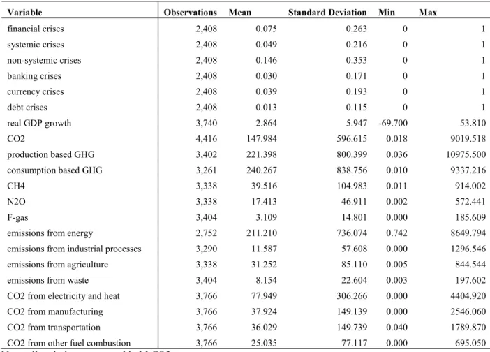
In addition, real GDP (in national currency) and real GDP growth are retrieved from the latest update of the IMFs World Economic Outlook (WEO) database, which covers 189 countries starting in 1980. For robustness purposes, we also use an indicator of the fiscal stance based on government’s consumption forecasts errors, retrieved from the October vintage of the WEO forecasts. Actual data on government consumption correspond to the first release. Summary statistics are presented in the Appendix Table A.1.
14 4.3 Event Study of Crises and Emissions
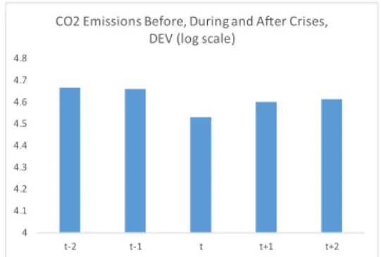
In Figure 1 we do a simple event-study exercise in which we plot the average level (in logs) of different types of emissions during, before and after a financial crisis. We do so by splitting the sample by country groups to inspect more closely heterogeneity given the underlying fundamental differences in economic structures and stages of development. In the first row we observe that financial crises to not seem to affect much the level of CO2 in Advanced Economies, but they increase in developing countries during t+1 and t+2. In Advanced Economies GHG emissions increase in the year of the crisis but they quickly return to lower levels afterwards. All other graphical results provide an unclear picture supporting the case for a serious econometric inspection that will follow.
Figure 1. Event Study of Emissions and Crises, AE vs DEV
4 4.1 4.2 4.3 4.4 4.5 4.6 4.7 4.8 t-2 t-1 t t+1 t+2
CO2 Emisisons Before, During and After Crises, AE (log scale) 4 4.1 4.2 4.3 4.4 4.5 4.6 4.7 4.8 t-2 t-1 t t+1 t+2
CO2 Emissions Before, During and After Crises, DEV (log scale)
15 5. Results
a. Baseline
Figure 2 presents the results obtained by estimating equation (1) for our six types of financial crises and for the four components of production-based GHG, namely CO2, N2O, CH4 and F-gas. Financial crises in general (top left panel) seem to lead to a statistically significant fall in CO2 and methane emissions (with the latter getting increasingly imprecisely estimated as the
4.2 4.4 4.6 4.8 5 5.2 5.4 t-2 t-1 t t+1 t+2
GHG Emisisons Before, During and After Crises, AE (log scale) 4.2 4.4 4.6 4.8 5 5.2 5.4 t-2 t-1 t t+1 t+2
GHG Emisisons Before, During and After Crises, DEV (log scale)
1.5 2 2.5 3 3.5 4 4.5 t-2 t-1 t t+1 t+2
Methane Emisisons Before, During and After Crises, AE (log scale)
1.5 2 2.5 3 3.5 4 4.5 t-2 t-1 t t+1 t+2
Methane Emisisons Before, During and After Crises, DEV (log scale)
1 1.5 2 2.5 3 3.5 t-2 t-1 t t+1 t+2
Nitrous Oxide Emisisons Before, During and After Crises, AE (log scale)
1 1.5 2 2.5 3 3.5 t-2 t-1 t t+1 t+2
Nitrous Oxide Emisisons Before, During and After Crises, DEV (log scale)
16
horizon expands). Magnitudes are non-negligible: a financial crisis can lead to the fall of up to 4 percent in CO2 emissions after 2 years (and slowly reducing to a fall of about 2 percent after 6
years).15 The fall in both CO2 and methane emissions is particularly sizeable when non-systemic
crises take place (top right panel). Turning to different types of crises, CO2 emissions also respond negatively and significantly following banking crises (a fall of up to 6 percent in these emissions in the medium-term), while methane and fluorinated gas react positively and significantly following debt crises (an increase of about 12 percent in these emissions in the medium-term). In all remaining cases, confidence bands do not allow us to state unequivocally that crises positively or negatively impacted a specific type of emissions.
17
Figure 2. Impulse Responses of GHG components to different financial crises, baseline, all countries
Figure 1.1. Effect of all Financial Crises
-10 -8 -6 -4 -2 0 2 4 -1 0 1 2 3 4 5 6 -6 -4 -2 0 2 4 6 -1 0 1 2 3 4 5 6 -3 -2 -1 0 1 2 3 4 5 6 -1 0 1 2 3 4 5 6
Figure 2.1. Effect of Systemic Crises
-6 -4 -2 0 2 4 6 8 -1 0 1 2 3 4 5 6 -20 -15 -10 -5 0 5 10 -1 0 1 2 3 4 5 6 -15 -10 -5 0 5 10 -1 0 1 2 3 4 5 6
Figure 3.1. Effect of Non Systemic Crises
-16 -14 -12 -10 -8 -6 -4 -2 0 2 -1 0 1 2 3 4 5 6 -6 -4 -2 0 2 4 -1 0 1 2 3 4 5 6 -8 -6 -4 -2 0 2 4 6 -1 0 1 2 3 4 5 6 -5 0 5 10 15 -1 0 1 2 3 4 5 6 1. CO2 (percent) 2. Methane (percent) 3. Nitrous Oxfide (percent) 4. Fluorinated Gas (percent) -60 -50 -40 -30 -20 -10 0 10 -1 0 1 2 3 4 5 6 -25 -20 -15 -10 -5 0 5 10 -1 0 1 2 3 4 5 6 1. CO2 (percent) 2. Methane (percent) 3. Nitrous Oxfide (percent) 4. Fluorinated Gas (percent) 1. CO2 (percent) 2. Methane (percent) 3. Nitrous Oxfide (percent) 4. Fluorinated Gas (percent)
Figure 4.1. Effect of Banking Crises
-16 -14 -12 -10 -8 -6 -4 -2 0 2 -1 0 1 2 3 4 5 6 -4 -2 0 2 4 6 8 -1 0 1 2 3 4 5 6 -3 -2 -1 0 1 2 3 4 5 6 -1 0 1 2 3 4 5 6
Figure 5.1. Effect of Currency Crises
-10 -5 0 5 10 15 -1 0 1 2 3 4 5 6 -8 -6 -4 -2 0 2 4 6 -1 0 1 2 3 4 5 6 -6 -4 -2 0 2 4 6 -1 0 1 2 3 4 5 6
Figure 6.1. Effect of Debt Crises
-25 -20 -15 -10 -5 0 5 10 -1 0 1 2 3 4 5 6 -10 -5 0 5 10 15 -1 0 1 2 3 4 5 6 -4 -2 0 2 4 6 8 10 12 -1 0 1 2 3 4 5 6 -20 -15 -10 -5 0 5 10 15 -1 0 1 2 3 4 5 6 -10 -5 0 5 10 15 20 25 -1 0 1 2 3 4 5 6 -10 -5 0 5 10 15 20 25 30 35 -1 0 1 2 3 4 5 6 1. CO2 (percent) 2. Methane (percent) 3. Nitrous Oxfide (percent) 4. Fluorinated Gas (percent) 1. CO2 (percent) 2. Methane (percent) 3. Nitrous Oxfide (percent) 4. Fluorinated Gas (percent) 1. CO2 (percent) 2. Methane (percent) 3. Nitrous Oxfide (percent) 4. Fluorinated Gas (percent)
18
Note: blue continuous line denotes the impulse response from equation 1. Dotted blue lines are the 90 percent confidence bands. The horizontal axis is expressed in annual frequency. t=0 is the starting year of a financial crisis.
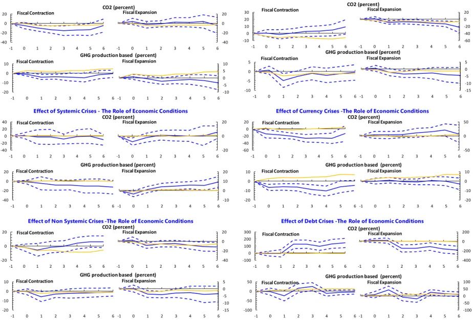
From this point onwards, only those IRFs yielding statistically significant results are show for reasons of parsimony (the full set of results is nonetheless available from the authors upon request). The previous set of unconditional effects mask, however, considerable variation depending on business cycle conditions, as shown by the OLS estimation of equation (2) reported in Figure 3.
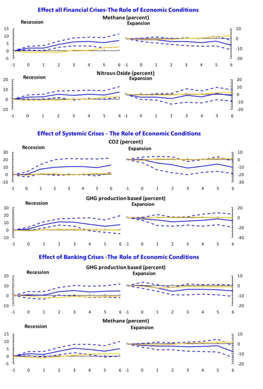
During periods of slack, financial crises in general seem to have a positive and statistically significant impact on both methane and nitrous oxide emissions (reaching about a 7 percent increase after 6 years). The reverse is true in good times (more so for the nitrous oxide), but the magnitude is not symmetric to that of bad times. Systemic crises that hit a country undergoing economic difficulties are associated with larger CO2 and production-based GHG. As for the type of financial crisis that seems to have larger impacts, yet again, debt crises are associated with increases in production based GHG emissions irrespectively of the phase of the business cycle. Also, methane, F-gas and nitrous oxide react positively in the short to medium-run following debt crises that take place during bad economic times. Under strong economic conditions however, financial crises seem to mildly lead to the reduction of various types of emissions, but the effects are not always precisely estimated.
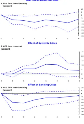
We also redid the previous analysis by focusing instead on economic sectors instead of gas nature. Such results are displayed in Figure A1 in the Appendix. They show that when hit by a debt crisis, a country experiences a rise in emissions stemming from either energy related activities or industrial processes. These effects are potentially large in the medium term and statistically
19
different from zero. In addition, relying on longer CO2 series, Figure A2 shows that carbon dioxide emissions emanating from manufacturing (transportation) decrease (increase) following a financial/banking (systemic) crisis.
20
Figure 3. Impulse Responses of Emissions to different financial crises, state contingent, all countries (selection)
Effect all Financial Crises-The Role of Economic Conditions Methane (percent) -5 0 5 10 15 -1 0 1 2 3 4 5 6 -20 -10 0 10 -1 0 1 2 3 4 5 6 Recession Expansion -10 0 10 20 -1 0 1 2 3 4 5 6 -20 -10 0 10 20 -1 0 1 2 3 4 5 6
Nitrous Oxide (percent)
Effect of Systemic Crises - The Role of Economic Conditions CO2 (percent) -10 0 10 20 30 -1 0 1 2 3 4 5 6 -30 -20 -10 0 10 -1 0 1 2 3 4 5 6
GHG production based (percent)
-10 0 10 20 30 -1 0 1 2 3 4 5 6 -40 -20 0 20 -1 0 1 2 3 4 5 6
GHG production based (percent)
Effect of Banking Crises -The Role of Economic Conditions
-10 0 10 20 -1 0 1 2 3 4 5 6 -20 -10 0 10 -1 0 1 2 3 4 5 6 -5 0 5 10 15 -1 0 1 2 3 4 5 6 -20 -10 0 10 -1 0 1 2 3 4 5 6 Methane (percent) -10 -20 Recession Expansion Recession Expansion Recession Expansion Recession Expansion Recession Expansion
21
Note: Blue continuous line denotes the impulse response from equation 2. Dotted blue lines are the 90 percent confidence bands. the yellow continuous line represents the unconditional baseline IRF from equation 1 (for comparison purposes). The horizontal axis is expressed in annual frequency. t=0 is the starting year of a financial crisis.
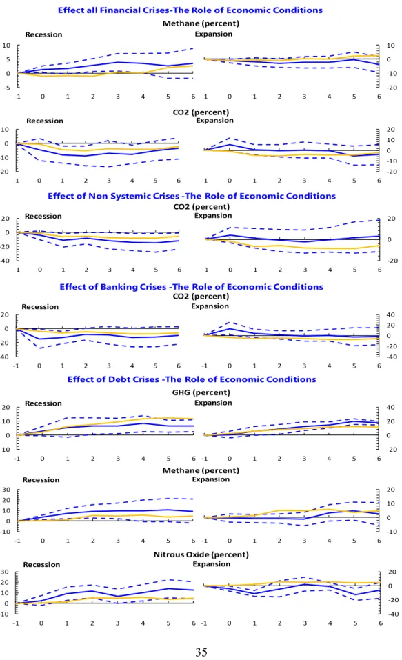
Next, we split between advanced economies and developing countries. Re-estimating equation 1 separately for each sub-sample yields the results displayed in Figures 4 and 5.
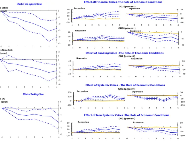
In Figure 4, left hand side panel, we observe that systemic and banking crises result in a fall in methane, nitrous oxide and production based GHG emissions in advanced economies in normal times. When we condition by the state of the economy, most types of crises (with the exception of currency and debt ones) are associated with a rise in emissions from CO2 and production based GHG during periods of economic slack, but their decline during booms.
Effect of Debt Crises -The Role of Economic Conditions GHG production based (percent)
Methane (percent)
Nitrous Oxide (percent)
Fluorinated Gas (percent)
-10 0 10 20 30 -1 0 1 2 3 4 5 6 -10 0 10 20 30 -1 0 1 2 3 4 5 6 0 10 20 30 -1 0 1 2 3 4 5 6 -20 -10 0 10 20 -1 0 1 2 3 4 5 6 -10 0 10 20 30 -1 0 1 2 3 4 5 6 -40 -20 0 20 40 -1 0 1 2 3 4 5 6 -20 0 20 40 60 -1 0 1 2 3 4 5 6 -60 -40 -20 0 20 -1 0 1 2 3 4 5 6 Methane (percent) Recession Expansion Recession Expansion Recession Expansion Recession Expansion
22
Evidence seems to suggest that in bad times, advanced economies do not take that opportunity to get away from carbon-intensive technologies and invest in cleaner ones, contrary to Papandreou’s (2015) argument.
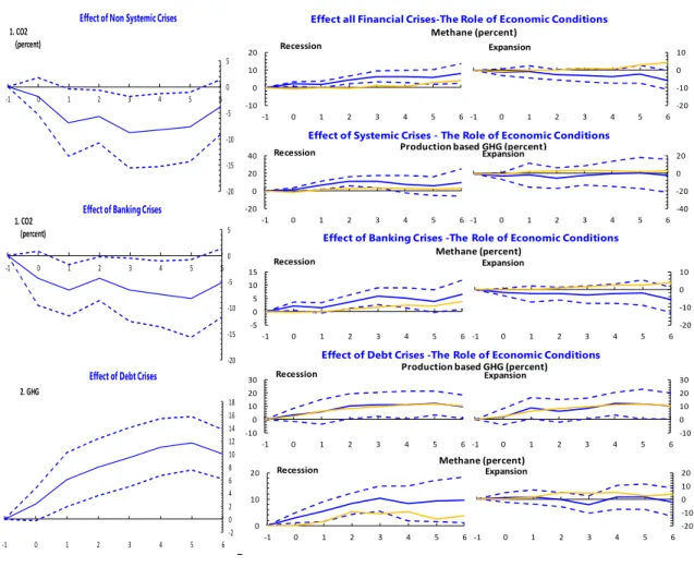
In Figure 5, the unconditional results for developing economies (left hand side panel) show negative (positive) and statistically significant response of CO2 (production based GHG) following systemic/banking (debt) crises. Estimating equation 2 for the subsample of developing economies shows a similar outcome in terms of a rise in emissions during bad times (but there CO2 is absent, i.e., results are statistically insignificant). In periods of strong economic conditions, most IRFs are not statistically different from zero (except the positive association between production based GHG and debt crises).
23
Figure 4. Impulse Responses of GHG components to different financial crises, baseline and state contingent, advanced economies (selection)
Note: Panel on the left includes the baseline estimation of equation 1 for the sample of advanced economies. Blue continuous line denotes the impulse response from equation 1. Dotted blue lines are the 90 percent confidence bands. Panel on the right include the state contingent estimation of equation 2 for the sample of advanced economies. Blue continuous line denotes the impulse response from equation 2. Dotted blue lines are the 90 percent confidence bands. the yellow continuous line represents the unconditional baseline IRF from equation 1 (for comparison purposes). The horizontal axis is expressed in annual frequency. t=0 is the starting year of a financial crisis.
Effect of Non Systemic Crises
-25 -20 -15 -10 -5 0 -1 0 1 2 3 4 5 6 -30 -25 -20 -15 -10 -5 0 5 10 -1 0 1 2 3 4 5 6 3. Methane (percent) 4. Nitrous Oxfide (percent)
Effect of Banking Crises
-20 -15 -10 -5 0 5 -1 0 1 2 3 4 5 6 2. GHG (percent) -10 0 10 20 30 -1 0 1 2 3 4 5 6 -40 -20 0 20 -1 0 1 2 3 4 5 6 -20 0 20 40 -1 0 1 2 3 4 5 6 -40 -20 0 -1 0 1 2 3 4 5 6 CO2 (percent) GHG (percent)
Effect all Financial Crises-The Role of Economic Conditions
Recession Expansion
Recession Expansion
Effect of Systemic Crises - The Role of Economic Conditions
-100 0 100 200 -1 0 1 2 3 4 5 6 -150 -100 -50 0 50 -1 0 1 2 3 4 5 6 CO2 (percent) GHG (percent) Recession Expansion Recession Expansion -20 0 20 40 60 -1 0 1 2 3 4 5 6 -100 -50 0 50 -1 0 1 2 3 4 5 6 CO2 (percent) Recession Expansion
Effect of Non Systemic Crises -The Role of Economic Conditions Effect of Banking Crises -The Role of Economic Conditions
-20 0 20 40 -1 0 1 2 3 4 5 6 -40 -20 0 20 -1 0 1 2 3 4 5 6
24
Figure 5. Impulse Responses of GHG components to different financial crises, baseline and state contingent, developing economies
Note: see note Figure 4.
b. Sensitivity and Robustness checks
Sensitivity
As shown by Tuelings and Zubanov (2010), a possible bias from estimating Equation (1) using country-fixed effects is that the error term of the equation may have a non-zero expected value, due to the interaction of fixed effects and country-specific fiscal developments. This would lead to a bias of the estimates that is a function of k. to address this issue and check the robustness of
Effect of Non Systemic Crises
1. CO2 (percent) -20 -15 -10 -5 0 5 -1 0 1 2 3 4 5 6
Effect of Banking Crises
-20 -15 -10 -5 0 5 -1 0 1 2 3 4 5 6 1. CO2 (percent)
Effect of Debt Crises
2. GHG (percent) -2 0 2 4 6 8 10 12 14 16 18 -1 0 1 2 3 4 5 6
Effect all Financial Crises-The Role of Economic Conditions
Methane (percent) -10 0 10 20 -1 0 1 2 3 4 5 6 -20 -10 0 10 -1 0 1 2 3 4 5 6 Effect of Systemic Crises - The Role of Economic Conditions
Production based GHG (percent)
-20 0 20 40 -1 0 1 2 3 4 5 6 -40 -20 0 20 -1 0 1 2 3 4 5 6 Effect of Banking Crises -The Role of Economic Conditions
Methane (percent) -5 0 5 10 15 -1 0 1 2 3 4 5 6 -20 -10 0 10 -1 0 1 2 3 4 5 6 Effect of Debt Crises -The Role of Economic Conditions
Production based GHG (percent)
Methane (percent) -10 0 10 20 30 -1 0 1 2 3 4 5 6 -10 0 10 20 30 -1 0 1 2 3 4 5 6 0 10 20 -1 0 1 2 3 4 5 6 -20 -10 0 10 20 -1 0 1 2 3 4 5 6 Recession Expansion Recession Expansion Recession Expansion Recession Expansion Recession Expansion
25
our findings, equation 1 was re-estimated by excluding country fixed effects from the analysis. The results (not shown but available upon request) suggest that this bias is negligible (the difference in the point estimate is small and not statistically significant).
As an additional sensitivity check, equation (1) was re-estimated for different lags (l) of the variables in the X vector. The results for zero lags, one lag and three lags (not shown but available upon request) confirm that previous findings are not sensitive to the choice of the number of lags. Robustness to the identification of slack
As an alternative variable measuring economic slack to use in the 𝐹(𝑧 ) function that enters equation 2, we have employed an output gap measure. Despite substantial progress in the estimation methodologies to calculate potential output, there is still not a widely accepted approach in the profession. According to Borio (2013), two alternative approaches to estimate potential GDP are used: i) there are univariate statistical approaches, which consist of filtering out the trend component from the cyclical one; ii) there are the structural approaches, which derive the estimates directly from the theoretical structure of a model. Aware of the shortcomings of using either one
or the other16, and at the cost of not maximizing the total number of observations in our panel
dataset, instead of relying on the IMF’s WEO measure of output gap17, we rather apply the recent
filtering technique developed by Hamilton (2017). In addition, we are also mindful of the criticisms surrounding the use of the popular Hodrick-Prescott (HP) filter (such as the identification of spurious cycles), particularly in the context of a large sample of very
16 Statistical methods suffer from the end-point problem, that is, they are extremely sensitive to the addition of new
data and to real-time data revisions. Structural models, on the other hand, may be difficult to implement consistently in cross-sectional environments and rely on the imposition of pre-determined assumptions.
17 The IMF does not have an official method for computing potential output and every country desk decides which
measure fits best. While the most common IMF approach uses a production function approach, assumptions vary greatly across countries and discretion is left to the country desks.
26
heterogeneous countries (Harvey and Jaeger, 1993; Cogley and Nason, 1995). Hamilton’s (2017)
approach to extract the cyclical and trend component of a generic variable
x
t (denoted x and ctt
x , respectively), consists of estimating:
𝑥 = 𝛾 + ∑ 𝛾 + 𝑥 + 𝑢 (3)
where xt xt xct.
The non-stationary part of the regression provides the cyclical component:
𝑥 = 𝑢 (4)
while the trend is given by
𝑥 = 𝛾 + ∑ 𝛾 + 𝑥 (5)
Hamilton (2017) suggests that h and k should be chosen such that the residuals from equation (3) are stationary and points out that, for a broad array of processes, the fourth differences of a series are indeed stationary. We choose h = 2 and k = 3, which is line with the dynamics seen in real GDP. Results of re-estimating equation 2 using the newly computed output gap as measure of slack, are displayed in Figure A3 in the appendix. We can see that while there are some similarities there are also some insightful differences with respect to the IRFs presented in Figure 3. We still get a positive (but weaker in significance) effect of financial crises in bad times on methane emissions. the differences are that CO2 emissions decline in times of economic strain after a financial crisis (particularly non-systemic and banking ones). Moreover, production based GHG emissions always reactive positively and significantly following a debt crisis irrespectively of the state of the economy. Finally, methane and nitrous oxide emissions increase after a debt crisis that hits the economic during periods of slack.
27 Does the prevailing fiscal stance matter?
The response of emissions to financial crises may also depend on whether the government is engaging in expansionary or contractionary fiscal policy at the time the economy is hit. To our knowledge, the only paper relating fiscal policy and the environment is the one by Lopez et al. (2011). The authors model (and empirically test) the impact of fiscal spending patterns on the environment and find that there is a reallocation of government spending composition towards social and public goods that tend to reduce pollution when an economy is hit by a negative shock. They further conclude that increasing total government spending (that is, engaging in expansionary fiscal policy) without altering its composition, does not reduce polluting emissions. while our setting is not identical, we still aim to shed further light into the effects of crises on the environment conditioning on prevailing (at the time of the shock) fiscal conditions. To this end, we consider an alternative version of equation 2 where instead of the state of the economy, we use instead an indicator of fiscal policy stance. The indicator fiscal policy stance is a government consumption shock, identified as the forecast error of government consumption expenditure relative to GDP (for
a similar approach see, e.g., Auerbach and Gorodnichenko 2012, 2013; and Abiad et al., 2015).18
Here, δ = 1 is used to assess the role of the fiscal policy.19 Figure 6 shows the results. Financial
crises hitting an economy when it is engaging in contractionary fiscal policies, leads to a negative and statistically significant response of CO2 and production-based emissions. In contrast, after systemic (non-systemic) crises that take place in periods of fiscal relaxation, production based GHG (CO2) emissions go up (down) in the medium term. Furthermore, CO2 emissions react negatively after banking and debt crises and a loosening of the fiscal stance. Finally, currency
18 This procedure also overcomes the problem of fiscal foresight (Forni and Gambetti 2010; Leeper et al., 2012, 2013;
Ben Zeev and Pappa 2014), because it aligns the economic agents’ and the econometrician’s information sets.
28
crises that take place at times of fiscal retrenchment lead to a fall in both CO2 and production based GHG emissions.
6. Conclusion
In this paper, we have provided empirical evidence on the impact of different types of financial crises on pollutant emissions for a sample of 86 countries between 1980-2012. We relied on the local projection method to plot the impulse responses of a variety of emissions categories (by type of gas and economic activity) to financial crises.
We found that financial crises in general led to a statistically significant fall in CO2 and methane emissions. CO2 emissions responded negatively and significantly following banking crises, while methane and fluorinated gas reacted positively and significantly following debt crises. Results also showed that production-based emissions increased following debt crises. Moreover, when hit by a debt crisis, a country experiences a rise in emissions stemming from either energy related activities or industrial processes. More specifically, CO2 emissions emanating from manufacturing (transportation) decrease (increase) following a financial/banking (systemic) crisis.
When we split the sample, we observed that, in normal times in advanced economies, systemic and banking crises resulted in a fall in methane, nitrous oxide and production based GHG emissions. In normal times in developing economies, systemic/banking (debt) crises resulted in a negative (positive) and statistically significant response of CO2 (production based GHG).
During periods of slack, financial crises in general had a positive and statistically significant impact on both methane and nitrous oxide emissions. Systemic crises that hit a country undergoing economic difficulties were associated with larger CO2 and production-based GHG. Debt crises were associated with increases in production based GHG emissions irrespectively of
29
the phase of the business cycle. Under strong economic conditions however, financial crises (weakly) led to the reduction of various types of emissions, but the effects were not always precisely estimated.
Finally, if a financial crisis hit an economy when it was engaging in contractionary fiscal policies, this led to a negative and statistically significant response of CO2 and production-based emissions. In contrast, after systemic (non-systemic) crises that took place in periods of fiscal relaxation, production based GHG (CO2) emissions went up (down) in the medium term. Furthermore, CO2 emissions reacted negatively after banking and debt crises and a loosening of the fiscal stance.
For policy makers, it is important so see financial crises as opportunities to make big reductions in emissions that one can then lock in, and ensure that carbon prices, investments and other policies nudge us all toward innovations that in turn give the tools to be a low carbon society, with a business model that combines prosperity with responsibility. As there is no one size fits all when it comes to policy implications (depends on development stage, initial conditions, current policy and institutional setting, political economy concerns, etc.) it is difficult to elaborate on country specific implications. This paper´s findings reinforce the need to improve economic and financial resilience to shocks as a way to prevent certain types of emissions to rise (as a result of a financial crisis). Hence, focus on macroprudential preventive regulation is a necessary component, while simultaneously countries with fiscal space should promote fiscal policies that support greener technologies (tax rebates, subsidies, deductions, etc.) so that the productive structure slowly transforms itself into a less pollutant one (with clear environmental sustainability positive externalities).
Figure 6. Impulse Responses of GHG components to different financial crises, state contingent, all countries -40 -20 0 20 -1 0 1 2 3 4 5 6 -40 -20 0 20 -1 0 1 2 3 4 5 6 -20 -10 0 10 -1 0 1 2 3 4 5 6 -10 -5 0 5 10 -1 0 1 2 3 4 5 6 CO2 (percent)
GHG production based (percent) Fiscal Contraction Fiscal Expansion
Fiscal Contraction Fiscal Expansion
Effect all Financial Crises-The Role of Economic Conditions
Effect of Systemic Crises - The Role of Economic Conditions
-40 -20 0 20 40 -1 0 1 2 3 4 5 6 -20 0 20 -1 0 1 2 3 4 5 6 -40 -20 0 20 -1 0 1 2 3 4 5 6 -10 0 10 20 -1 0 1 2 3 4 5 6
Effect of Non Systemic Crises -The Role of Economic Conditions
-20 0 20 -1 0 1 2 3 4 5 6 -40 -20 0 20 -1 0 1 2 3 4 5 6 -20 -10 0 10 -1 0 1 2 3 4 5 6 -15 -10 -5 0 5 -1 0 1 2 3 4 5 6
Effect of Banking Crises -The Role of Economic Conditions
-10 0 10 20 30 -1 0 1 2 3 4 5 6 -60 -40 -20 0 20 -1 0 1 2 3 4 5 6 -10 -5 0 5 -1 0 1 2 3 4 5 6 -15 -10 -5 0 5 -1 0 1 2 3 4 5 6
Effect of Currency Crises -The Role of Economic Conditions
-60 -40 -20 0 20 -1 0 1 2 3 4 5 6 -50 0 50 -1 0 1 2 3 4 5 6 -20 -10 0 10 -1 0 1 2 3 4 5 6 -20 -10 0 10 -1 0 1 2 3 4 5 6
Effect of Debt Crises -The Role of Economic Conditions
-100 0 100 200 300 -1 0 1 2 3 4 5 6 -400 -200 0 200 -1 0 1 2 3 4 5 6 -100 -50 0 50 -1 0 1 2 3 4 5 6 -100 -50 0 50 100 -1 0 1 2 3 4 5 6 CO2 (percent)
GHG production based (percent) Fiscal Contraction Fiscal Expansion
Fiscal Contraction Fiscal Expansion
CO2 (percent)
GHG production based (percent) Fiscal Contraction Fiscal Expansion
Fiscal Contraction Fiscal Expansion
CO2 (percent)
GHG production based (percent) Fiscal Contraction Fiscal Expansion
Fiscal Contraction Fiscal Expansion CO2 (percent)
GHG production based (percent) Fiscal Contraction Fiscal Expansion
Fiscal Contraction Fiscal Expansion CO2 (percent)
GHG production based (percent) Fiscal Contraction Fiscal Expansion
References
1. Abiad, A., Furceri, D., Topalova, P. (2015), “The Macroeconomic effects of public investment: evidence from Advanced Economies”, IMF WP 15/95. Washington DC. 2. Acemoglu, D. and J. Robinson (2012), “Why Nations Fail: The origins of power, prosperity
and Poverty”, Crown Business
3. Ajmi, A., S. Hammoudeh, D. Nguyen, and J. Sato. (2015). “On the Relationships between CO2 Emissions, Energy Consumption and Income: The Importance of Time Variation”. Energy Economics 49 (May): 629–38.
4. Amann, M., Cofala, J., Rafaj, P, Wagner, F. (2009), “The Impact of the economic crises on GHG mitigation and costs in Annex I countries”, International Institute for Applied Systems Analysis.
5. Auerbach, A., and Y. Gorodnichenko (2012), “Fiscal Multipliers in Recession and Expansion.” In Fiscal Policy After the Financial Crisis, eds. Alberto Alesina and Francesco Giavazzi, NBER Books, National Bureau of Economic Research, Inc., Cambridge, Massachusetts.
6. Auerbach, A., and Y. Gorodnichenko (2013), “Measuring the Output Responses to Fiscal Policy.” American Economic Journal: Economic Policy 4 (2): 1–27.
7. Ball, L. Furceri, D., Leigh, D., Loungani, P. (2013), “The distributional effects of fiscal consolidation”, IMF WP 13/151, Washington DC.
8. Ben Zeev, N., and E. Pappa (2014), “Chronicle of a War Foretold: The Macroeconomic Effects of Anticipated Defense Spending Shocks.” CEPR Discussion Paper 9948, Centre for Economic Policy Research, London.
9. Cai, X. and W. Den Haan (2009), “Predicting recoveries and the importance of using enough information,” CEPR Discussion Paper, No. 7508.
10. Cerra, V. and S. C. Saxena (2008) “Growth Dynamics: The Myth of Economic Recovery,” American Economic Review, 98(1), 439-457.
11. Cogley, T. and J. Nason (1995), “Effects of the Hodrick-Prescott filter on trend and difference stationary time series Implications for business cycle research,” Journal of Economic Dynamics and Control, 19(1-2), 253- 278.
12. Cohen, G., Jalles, J., Marto, R., Loungani, P. (2018), “The Long-Run Decoupling of Emissions and Output: Evidence from the Largest Emitters”, Energy Policy (forthcoming) 13. Declercq, B., Delarue, E. and D`haeseleer, W. (2011), “Impact of the economic recession
on the European power sector’s CO2 emissions”. Energy Policy, 39, pp. 1677-1686. 14. Del Río, P.and Labandeira, X. (2009), “Climate change at times of economic crisis”,
FEDEA Coleccion Estudios Economicos, 05-09.
15. Doda, B. (2014), “Evidence on Business Cycles and CO2 Emissions”. Journal of Macroeconomics 40, 214-227
16. Egenhofer, C. (2008), “Climate change policy after the financial crisis: The latest excuse for a new round of state aid?”, CEPS Commentary/30 October 2008, Brussels
17. Ericsson, N. R., D. F. Hendry, and K. M. Prestwich (1997), “The Demand for Broad Money in the United Kingdom, 1878-1993,” International Finance Discussion Papers, No. 596. 18. Forni, M., and L. Gambetti (2010), “Fiscal Foresight and the Effects of Government
32
19. Geels, F. (2013), “The impact of the financial-economic crisis on sustainability transitions: financial investment, governance and public discourse”, Environmental Innovation and Societal Transitions, 6, 67-95.
20. Geels, F. W. (2002), “Technological transitions as evolutionary reconfiguration processes: a multi-level perspective and a case-study”, Research Policy, 31(8), 1257-1274.
21. Gierdraitis, V., Girdenas, S., and Rovas, A. (2010), “Feeling the heat: Financial crises and their impact on global climate change”, Perspectives of Innovations, Economics and Business, 4(1), 7-10.
22. Granger, C. W. J., and T. Teräsvirta (1993), “Modelling Nonlinear Economic Relationships”. New York: Oxford University Press.
23. Greenpeace (2008), “Energy[r]evolution. A Sustainable EU-27 Energy Outlook”. Greenpeace International. November 2008.
24. Hamilton, J. (2017), “Why You Should Never Use the Hodrick-Prescott Filter,” NBER WP paper No. 23429.
25. Harvey, A. and A. Jaeger (1993), “Detrending, Stylized Facts and the Business Cycle,” Journal of Applied Econometrics, 8(3), 231-47.
26. Hendry, D. (1995), “Dynamic econometrics”, Oxford: Oxford University Press.
27. Hordijk, L. and M. Amann (2007), “How Science and Policy Combined to Combat Air Pollution Problems”, Environmental Policy and Law, 37(4): 336-340.
28. IEA. (2013). Tracking clean energy progress 2013. International Energy Agency.
29. Jaunky, V. C. (2010), “The CO2 emission-income nexus: Evidence from rich countries”. Energy Policy, 39, 1228-1240.
30. Jordà, O. (2005), “Estimation and Inference of Impulse Responses by Local Projections.” American Economic Review 95 (1): 161–82.
31. Kaika, D. and Zervas, E. (2013a). “The Environmental Kuznets Curve (EKC) theory — Part A: Concept, causes and the CO2 emissions case”. Energy Policy 62, 1392–1402. 32. Kaika, D. and Zervas, E. (2013b). “The Environmental Kuznets Curve (EKC) theory —
Part B: Critical issues”. Energy Policy 62, 1403–1411.
33. Kriström, B. and T. Lundgren (2005), “Swedish CO2 Emissions 1900-2100 – An Exploratory Note”, Energy Policy, 33, 1223-1230.
34. Laeven, L. and F. Valencia, 2010, “Resolution of Banking Crises: The Good, the Bad, and the Ugly,” IMF Working Paper No. 10/44.
35. Lane, J.-E. (2011), “CO2 emissions and GDP”. International Journal of Social Economics, 38, 911- 918.
36. Leeper, E. M., A. W. Richter, and T. B. Walker (2012), “Quantitative Effects of Fiscal Foresight.” American Economic Journal: Economic Policy 4 (2): 115– 44.
37. Leeper, E. M., T. B. Walker, and S. S. Yang (2013), “Fiscal Foresight and Information Flows.” Econometrica 81 (3): 1115–45.
38. Leichenko, R. M., O'Brien, K. L., and Solecki, W. D. (2010). Climate Change and the Global Financial Crisis: A Case of Double Exposure. Annals of the Association of American Geographers, 100, 963-972.
39. Marechal, K. (2007), “The economics of climate change and the change of climate in economics”, Energy Policy, 35, 5181-5194.
40. Nickell, S. (1981). “Biases in dynamic models with fixed effects”. Econometrica, 1417-1426.
33
41. Papandreou, A. (2015), “The Great Recession and the transition to a low-carbon economy”, Working Paper No. 88, Financialisation, Economy, Society & Sustainable Development Project.
42. Peters, G. P., and E. G. Hertwich (2008), “CO2 embodied in international trade with implications for global climate policy”, Environmental Science Technology, 42, 1401 – 1407
43. Peters, G. P., Marland, G., Le Quéré, C., Boden, T., Canadell, J. G., and Raupach, M. R. (2011)., “Rapid growth in CO2 emissions after the 2008-2009 global financial crisis”. Nature Climate Change, 2(1), 2-4.
44. Romer, C. D. and D. H. Romer (1989), “Does Monetary Policy Matter? A New Test in the Spirit of Friedman and Schwartz,” NBER Macroeconomic Annual, 4, 121-184.
45. Siddiqi, T. A. (2000), “The Asian Financial Crisis: is it good for the global environment?”, Environmental Change, 10, 1-7.
46. Sobrino, N. and Monzon, A. (2014), “The impact of the economic crisis and policy actions on GHG emissions from road transport in Spain”, Energy Policy, 74, pp. 486-498.
47. Stavytskyy, A., Giedraitis, V., Sakalauskas, D., and Huettinger, M. (2016), “Economic crises and emission of pollutants: a historical review of selected economies amid two economic recessions”, Ekonomia, 95(1).
48. Stern, D. I. (2004), “The rise and fall of the environmental Kuznets curve”, World Development. 32 (8), 1419–1439.
49. Teulings, C. and N. Zubanov (2010), “Economic Recovery a Myth? Robust Estimation of Impulse Responses,” CEPR Discussion Paper 7300 (London: CEPR).
50. Tuinstra, W. (2007), “Preparing for the European Thematic Strategy on air pollution: at the interface between science and policy”, Environmental Science and Policy 10(5): 434- 444. 51. Unruh, G., (2000), “Understanding carbon lock-in”. Energy Policy 28, 817–830.
52. Van Bree, B., Verbong, G.P.J., Kramer, G. J. (2010), “A multi-level perspective on the introduction of hydrogen and battery-electric vehicles”. Technological Forecasting and Social Change 77, 529–540
53. Wooders, P. and Runnals, D. (2008), “The Financial Crisis and Our Response to Climate Change”. An IISD Commentary.
54. York, R. (2012), “Asymmetric effects of economic growth and decline on CO2 emissions”, Nature Climate Change. 2(11). p762-764.
34 APPENDIX
Figure A1. Impulse Responses of Emissions to different financial crises, emissions by economic sector, all countries
Figure A2. Impulse Responses of Emissions to different financial crises, CO2 emissions by type of activity, all countries
Effect of Debt Crises
1. Emissions from energy (percent)
2. Emissions from industrial processes (percent) -5 0 5 10 15 20 25 -1 0 1 2 3 4 5 6 0 10 20 30 40 50 -1 0 1 2 3 4 5 6
2. CO2 from manufacturing (percent) -35 -30 -25 -20 -15 -10 -5 0 5 10 -1 0 1 2 3 4 5 6
Effect of all Financial Crises
3. CO2 from transport (percent) -5 0 5 10 15 20 25 -1 0 1 2 3 4 5 6
Effect of Systemic Crises
Effect of Banking Crises
-35 -30 -25 -20 -15 -10 -5 0 5 10 -1 0 1 2 3 4 5 6
2. CO2 from manufacturing (percent)
35
Figure A3. Impulse Responses of Emissions to different financial crises, state contingent using alternative measure of slack (Hamilton, 2017 filter), all countries
Effect all Financial Crises-The Role of Economic Conditions
Recession Expansion Methane (percent) -5 0 5 10 -1 0 1 2 3 4 5 6 -20 -10 0 10 -1 0 1 2 3 4 5 6 CO2 (percent) -20 -10 0 10 -1 0 1 2 3 4 5 6 -20 -10 0 10 20 -1 0 1 2 3 4 5 6 Recession Expansion
Effect of Non Systemic Crises -The Role of Economic Conditions CO2 (percent) -40 -20 0 20 -1 0 1 2 3 4 5 6 -20 0 20 -1 0 1 2 3 4 5 6 Recession Expansion
Effect of Banking Crises -The Role of Economic Conditions CO2 (percent) Recession Expansion -40 -20 0 20 -1 0 1 2 3 4 5 6 -40 -20 0 20 40 -1 0 1 2 3 4 5 6 GHG (percent)
Effect of Debt Crises -The Role of Economic Conditions
-10 0 10 20 -1 0 1 2 3 4 5 6 -20 0 20 40 -1 0 1 2 3 4 5 6 Recession Expansion Methane (percent) Recession Expansion -10 0 10 20 30 -1 0 1 2 3 4 5 6 -10 0 10 20 -1 0 1 2 3 4 5 6
Nitrous Oxide (percent)
Recession Expansion -10 0 10 20 30 -1 0 1 2 3 4 5 6 -40 -20 0 20 -1 0 1 2 3 4 5 6
36
Table A1. Summary Statistics
Variable Observations Mean Standard Deviation Min Max
financial crises 2,408 0.075 0.263 0 1 systemic crises 2,408 0.049 0.216 0 1 non-systemic crises 2,408 0.146 0.353 0 1 banking crises 2,408 0.030 0.171 0 1 currency crises 2,408 0.039 0.193 0 1 debt crises 2,408 0.013 0.115 0 1 real GDP growth 3,740 2.864 5.947 -69.700 53.810 CO2 4,416 147.984 596.615 0.018 9019.518 production based GHG 3,402 221.398 800.399 0.036 10975.500 consumption based GHG 3,261 240.267 838.756 0.010 9337.216 CH4 3,338 39.516 104.983 0.011 914.002 N2O 3,338 17.413 46.911 0.002 572.441 F-gas 3,404 3.109 14.801 0.000 185.609
emissions from energy 2,752 211.210 736.074 0.742 8649.794 emissions from industrial processes 3,290 11.587 57.608 0.000 1296.546 emissions from agriculture 3,338 31.252 85.110 0.005 844.544 emissions from waste 3,404 8.154 22.604 0.003 197.602 CO2 from electricity and heat 3,766 77.949 306.266 0.000 4404.920 CO2 from manufacturing 3,766 37.924 149.139 0.000 2546.060 CO2 from transportation 3,766 36.029 149.739 0.040 1789.870 CO2 from other fuel combustion 3,766 25.035 77.117 0.000 695.050
37
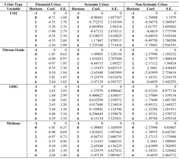
Table A2. Regression Results underlying Figure 2
Crisis Type Financial Crises Systemic Crises Non-Systemic Crises Variable Horizon Coef. S.E. Horizon Coef. S.E. Horizon Coef. S.E.
CO2 -1 0 0 -1 0 0 -1 0 0 0 -0.71 1.68 0 -0.90441 1.057367 0 -1.76888 1.7479 1 -4.53 1.78 1 0.772272 2.316384 1 -6.54578 3.360587 2 -5.28 2.35 2 0.883894 2.96218 2 -5.61757 2.695062 3 -3.90 2.79 3 -0.67152 2.674513 3 -8.0619 3.775799 4 -4.33 2.34 4 0.328073 2.610025 4 -8.64919 3.858104 5 -4.33 2.60 5 1.17447 2.870513 5 -8.49758 3.780209 6 -2.36 2.80 6 1.235166 2.713416 6 -5.73042 2.936191 Nitrous Oxide -1 0 0 -1 0 0 -1 0 0 0 -1.01 0.63 0 -1.09885 1.528136 0 -2.37996 1.103232 1 -0.90 0.97 1 1.835653 2.707504 1 -1.78975 1.408438 2 -0.97 1.95 2 -0.84715 2.98527 2 -2.17112 1.98824 3 0.35 2.30 3 -1.31435 4.682515 3 -2.3841 2.436445 4 0.10 1.84 4 -2.65448 5.603994 4 -2.61899 2.724618 5 2.01 1.87 5 -5.25579 5.631676 5 -1.34331 3.210178 6 2.64 1.65 6 -5.47139 6.595737 6 -0.6659 3.442593 GHG -1 0 0 -1 0 0 -1 0 0 0 2.63 2.85 0 -1.37979 0.890642 0 -0.51243 0.977136 1 1.84 2.99 1 0.400627 2.636837 1 -2.37006 1.559154 2 1.48 3.02 2 0.632599 2.339572 2 -1.77698 1.691703 3 2.65 3.20 3 0.917608 2.136018 3 -0.89121 2.168527 4 2.68 3.30 4 0.150942 3.124706 4 -1.32284 2.281911 5 4.08 3.34 5 0.296645 3.559678 5 -1.55331 2.570712 6 4.39 3.54 6 -0.13134 3.523921 6 -1.29786 2.659318 Methane -1 0 0 -1 0 0 -1 0 0 0 -1.01 0.37 0 -1.09885 1.103059 0 -2.37996 0.85067 1 -0.90 0.69 1 1.835653 1.997665 1 -1.78975 0.645781 2 -0.97 0.73 2 -0.84715 2.400755 2 -2.17112 1.173948 3 0.35 0.96 3 -1.31435 3.060335 3 -2.3841 1.580965 4 0.10 1.09 4 -2.65448 4.136325 4 -2.61899 1.782092 5 2.01 1.34 5 -5.25579 4.627652 5 -1.34331 2.328402 6 2.64 1.40 6 -5.47139 5.005467 6 -0.6659 2.464712
38
(cont.)
Crisis Type Banking Crises Currency Crises Debt Crises
Variable Horizon Coef. S.E. Horizon Coef. S.E. Horizon Coef. S.E.
CO2 -1 0 0 -1 0 0 -1 0 0 0 -3.80212 2.589324 0 1.66637 1.725489 0 0.150624 1.963288 1 -5.87962 2.406554 1 -1.47369 1.769458 1 -3.66276 3.458048 2 -4.56673 2.107138 2 -3.28143 3.485882 2 -4.71787 3.983103 3 -5.99366 3.124376 3 0.065792 3.053412 3 -5.23135 4.524772 4 -7.46269 3.205056 4 0.463461 2.887159 4 -2.61295 4.527835 5 -7.93038 3.860955 5 2.869655 2.803182 5 -4.39965 6.420521 6 -6.01086 3.446878 6 4.652825 2.845627 6 -7.39872 6.936317 Nitrous Oxide -1 0 0 -1 0 0 -1 0 0 0 -0.80921 0.729287 0 -1.71099 0.83935 0 0.236698 1.812968 1 -1.21593 1.027824 1 -0.60392 1.317535 1 1.514265 3.462669 2 -0.41014 1.452431 2 -2.1012 2.701583 2 5.194294 3.132698 3 0.604175 1.824026 3 -0.94348 3.278729 3 4.718475 3.128873 4 1.33193 2.06327 4 -2.46193 2.554982 4 5.681625 3.400002 5 1.602326 2.434544 5 0.51329 2.719101 5 3.687199 4.910997 6 1.715606 2.71248 6 0.945725 2.108958 6 4.772572 4.727071 GHG -1 0 0 -1 0 0 -1 0 0 0 -0.51519 0.75696 0 2.759019 4.188067 0 2.301983 1.41463 1 -2.22241 1.053105 1 3.716023 4.2982 1 5.998375 2.391651 2 -1.90463 1.197318 2 3.423266 4.344099 2 7.753236 2.296185 3 -0.82515 1.549602 3 4.115162 4.577513 3 9.57633 2.338375 4 -1.37045 1.661871 4 4.602129 4.698332 4 11.56606 2.065934 5 -1.1818 1.88728 5 7.122493 4.731679 5 12.39219 2.073119 6 -1.24582 2.063264 6 6.939784 4.808266 6 11.52471 1.841711 Methane -1 0 0 -1 0 0 -1 0 0 0 -0.80921 0.417815 0 -1.71099 0.529014 0 0.236698 0.99905 1 -1.21593 0.758213 1 -0.60392 0.650377 1 1.514265 2.084379 2 -0.41014 0.921955 2 -2.1012 0.920469 2 5.194294 2.447521 3 0.604175 1.250166 3 -0.94348 1.341592 3 4.718475 2.697006 4 1.33193 1.505258 4 -2.46193 1.547163 4 5.681625 3.377401 5 1.602326 1.878642 5 0.51329 1.935123 5 3.687199 3.601817 6 1.715606 1.99962 6 0.945725 1.992354 6 4.772572 3.77971 Note: horizon denotes the k-period ahead. “coef” and “S.E.” denote the coefficient estimate and corresponding standard error estimated in equation 1.