Dynamic functional connectivity of BOLD fMRI signal during both rest and task execution states

(1)

Universidade de Lisboa

Faculdade de Ciências

Departamento de Física

Dynamic Functional Connectivity of BOLD fMRI

signal during both rest and task execution states

Joana Paula Fontinha de Brito

Dissertação

Mestrado Integrado em Engenharia Biomédica e Biofísica

Perfil em Engenharia Clínica e Instrumentação Médica

(2)

Universidade de Lisboa

Faculdade de Ciências

Departamento de Física

Dynamic Functional Connectivity of BOLD fMRI

signal during both rest and task execution states

Joana Paula Fontinha de Brito

Dissertação

Mestrado Integrado em Engenharia Biomédica e Biofísica

Perfil em Engenharia Clínica e Instrumentação Médica

Orientadores: Professor Alexandre Andrade e Professor Hugo Ferreira

(3)

i

ACKNOWLEDGMENTS

First of all, I would like to thank to my professors, Alexandre Andrade and Hugo Ferreira, for all the patience, help, availability and learning through my academic journey. Their collaboration was, undoubtedly, very important to me.

I also would like to thank to the Institute of Biophysics and Biomedical Engineering for hosting me during the last years and to the Technical University of Graz for kindly made available all the subjects datasets used on this work.

To my parents, Maria de Fátima Fontinha and Armando Brito I would like to say how grateful I am for all the attention, the emotional support and for all the friendly words of encouragement. With the same love I mention my brother, João Brito, whom I thank for all the silly jokes and chocolate cakes that always animate me. It would not be fair to forget my lovely pet, named Békita, for waking me up with kisses and salute me every day with the same affection and joy. I also would like to thank to my grandmother Idolinda for all the education and prayers in my name.

A special thankful to my best friend and sister, Vânia, with whom I shared so many moments. One of the most important things that I carry from my academic life is our friendship. I am deeply thankful to you for always being there for me.

I don't want to forget anyone so I would like to thank to all people who somehow contribute and help me. I consider my academic journey and my personal journey as our journey.

And, although you are no longer with us, I not only thank you, but also dedicate all my work, all my effort and all my wins up to today. I know you are smiling for me. I will miss you forever.

This research was supported by Fundação para a Ciência e Tecnologia (FCT) and Ministério da Ciência e Educação (MCE) Portugal (PIDDAC) under grants PTDC/SAU-ENB/120718/2010 and PEst-OE/SAU/UI0645/2014.

"

Gratitude is the only treasure of the humble"

William Shakespeare

(4)

ii

RESUMO

A conectividade cerebral é um tema muito atual na área das neurociências. A dinâmica da conectividade tem sido um tema muito explorado ultimamente com o objetivo de se descobrir mais sobre os processos cerebrais relacionados com sinais neuronais em bandas restritas de frequência e ainda compreender as diferenças entre repouso e execução de tarefas. O objetivo principal do presente trabalho consistiu no desenvolvimento de um procedimento para o estudo da conectividade dinâmica baseado na análise da coerência através da Transformada "Wavelet" que proporciona especificidade no tempo e na frequência. A abordagem implementada baseou-se em duas hipótebaseou-ses diferentes de comunicação neuronal. A primeira considera que dois sinais neuronais oscilatórios comunicam durante períodos de coerência de magnitude elevada e a segunda considera que a comunicação neuronal ocorre em períodos de acoplamento de fase. O uso das duas hipóteses permitiu obter, respectivamente, dois perfis de comunicação neuronal. Uma vez que, as distribuições nulas dos perfis de coerência de magnitude e de acoplamento de fase são desconhecidas, e que os dados provêm de "single-trials" (ou seja, provêm de experiências únicas, sem repetição para um mesmo estado) foi construído um teste estatístico baseado em simulação de dados. A partir deste teste foi possível, para um dado nível de significância, distinguir períodos de comunicação neuronal significativa. Como a interação entre cada par de regiões é analisada através de janelas temporais, ao longo das séries temporais, os períodos de comunicação significativa correspondem a janelas onde há interação. Para os períodos de comunicação significativa foi calculado um valor médio de atraso temporal. A informação obtida a partir do método implementado pode ser expressa sob a forma de matrizes de conectividade funcional para todas as regiões do cérebro e sub-matrizes para regiões pertencentes a redes cerebrais específicas, usando ambas as medidas de comunicação como métricas de conectividade. Este método origina também mapas cerebrais para uma análise baseada numa região de referência onde são apresentados, através de mapas de cores, os valores médios de atrasos temporais entre a região referência e todas as restantes regiões do cérebro, ou para um conjunto mais específico. A partir da análise dos valores médios de atrasos temporais é possível estabelecer uma cronometria da passagem de informação. Se o valor obtido para o atraso temporal entre a região A e a região B é positivo, então, a região A é ativada primeiro e considera-se que precede a região B. A partir deste método é obtida uma análise detalhada entre cada duas regiões cerebrais através da observação dos perfis de interação para as duas hipóteses de comunicação neuronal e pela observação das distribuições de fases e atrasos temporais nas janelas de comunicação. Em relação às distribuições de fase um dos objetivos é conseguir identificar casos em que haja intervalos de fase preferidos para comunicação. A análise dos perfis de coerência de magnitude e acoplamento de fase permitem constatar que há flutuações

(5)

iii na comunicação ao longo das várias janelas temporais o que demostra uma dinâmica na conectividade funcional. Para ambos os perfis foi feita uma análise de correlação e de informação mútua. Para todos os casos analisados concluiu-se que há uma forte semelhança entre as medidas de coerência de magnitude e acoplamento de fase ao longo de todas as janelas temporais, com e sem comunicação significativa. Para testar e ilustrar a metodologia desenvolvida utilizou-se um conjunto de dados de três sujeitos, pelo que não há intenção de formalizar conclusões universais sobre a dinâmica de conectividade cerebral. Para todos os sujeitos a análise focou-se numa gama restrita de frequências, centrada nos 0.1 Hz, de forma a estudar a dinâmica da conectividade ao nível das oscilações lentas da resposta BOLD ("Blood Oxygenation Level-Dependent") que é obtida através de Ressonância Magnética funcional. Estas oscilações estão identificadas como características destes sinais, no entanto, a sua origem ainda não foi descoberta, o que causa um grande interesse na sua exploração.

Ao nível de significância de 95% os resultados mostram uma forte correlação positiva entre as duas métricas de comunicação utilizadas. Em relação á análise de informação mútua, entre as duas variáveis de comunicação, concluiu-se que ambos os perfis contêm 80% de informação comum. Os dados utilizados consistem num paradigma com aquisição em repouso e durante a execução do movimento de um dedo de forma voluntária e de forma estimulada, através de um estímulo auditivo. As matrizes de conectividade obtidas para os três sujeitos, durante todos os momentos de aquisição, e para as duas medidas de conectividade estudadas, revelam uma maior interação global entre as regiões cerebrais para os momentos de execução de tarefa do que para os momentos de repouso. Ou seja, maiores valores de conectividade funcional, para ambas as variáveis estudadas, entre um maior número de regiões para movimento voluntário e estimulado do que para repouso. Uma análise mais pormenorizada em regiões pertencentes à rede motora frontal-cognitiva e á rede parietal-premotora, ambas associadas ao movimento, mostram interações muito elevadas para ambos os movimentos, em todos os sujeitos analisados. Na análise mais detalhada entre regiões específicas, para dois sujeitos em movimento voluntário, detectou-se que os valores obtidos de fase entre a região motora primária esquerda, SMA, e o cíngulo anterior bem como a insula anterior, estão confinados ao intervalo durante as janelas temporais de comunicação, sugerindo uma preferência nos valores de fase para ambas as hipóteses de comunicação neuronal. Em relação ao estabelecimento da cronometria da passagem de informação entre regiões cerebrais, obteve-se, para todos os sujeitos, que a ínsula é ativada primeiro que o SMA durante as duas aquisições de execução de tarefa. Para dois dos três sujeitos analisados obteve-se, em movimento voluntário, que os gânglios da base, também envolvidos no controlo motor, são ativados antes da área SMA, pelo que a passagem de informação ocorre nesse sentido, como já foi reportado em estudos anteriores. Um tópico muito interessante e que tem sido o centro de muita discussão científica recai sobre a causa dos atrasos

(6)

iv temporais em fMRI. O grande foco tem sido sobre estes atrasos se deverem a diferenças hemodinâmicas ou a diferenças neuronais. O método implementado e apresentado neste trabalho não permite uma análise direta sobre este assunto mas, apesar de não fornecer uma forma de distinguir as duas hipóteses, alguns dos resultados obtidos corroboram a hipótese de que os atrasos temporais têm origem neuronal. A obtenção de diferentes latências entre as aquisições em repouso e as aquisições durante a execução de tarefas, de forma voluntária e estimulada, apoiam a hipótese de que os atrasos temporais não se devem apenas a atrasos hemodinâmicos. Se os resultados temporais apenas se devessem a atrasos hemodinâmicos, então, não seriam esperadas diferenças entre os valores obtidos para repouso e execução de tarefa. Também a descoberta de atrasos temporais diferentes entre regiões homólogas, em repouso e tarefa, apoia a ideia da origem neuronal uma vez que, seria esperado que os parâmetros fisiológicos que governam as latências hemodinâmicas fossem comparáveis entre regiões homólogas (e regiões vizinhas), com suplemento arterial e drenagem venosa comum.

A partir da metodologia implementada foi possível analisar redes cerebrais relacionadas com repouso, movimento voluntário e movimento estimulado, em termos de períodos de comunicação neuronal e atrasos temporais. Uma vez que, há consistência entre resultados obtidos com a abordagem utilizada e resultados descritos na bibliografia, conclui-se que a metodologia implementada para análise da conectividade funcional foi bem sucedida. Para concluir, de forma a melhorar e complementar o método desenvolvido, outras análises podem ser aplicadas, como uma análise de "clustering" (ou seja, uma análise de agrupamento) de forma a agrupar regiões cerebrais com perfis de comunicação semelhantes ou uma análise de periodicidade para analisar periodicidades nas flutuações dos mesmos perfis. De forma a complementar este método também medidas de conectividade anatómica e efetiva devem ser exploradas.

PALAVRAS-CHAVE

Conectividade dinâmica, Comunicação neuronal, BOLD fMRI, Oscilações lentas, Coerência Wavelet.

(7)

v

ABSTRACT

Brain connectivity is a very active topic in neuroscience. The main goal of the present work consisted on the development of a dynamic connectivity procedure based on wavelet coherence analysis which provides time-frequency specificity. The implemented approach was based on two different neuronal communication hypotheses. One considering that two oscillating neural signals communicate during periods of high magnitude coherence and the other considering that neuronal communication occurs during phase locking periods. Using both hypotheses two different profiles of neuronal communication were obtained. To deal with unknown null distributions, for single-trial data, a surrogate- based statistical test was performed to distinguish significant periods of communication. For those periods, an averaged temporal delay was computed. To test and illustrate the developed methodology a three subjects dataset is used including resting, voluntary and stimulus-driven action states. From functional connectivity matrices it is observed higher global interaction for both action conditions than for resting state. During tasks both frontal-cognitive and parietal-premotor networks have high connectivity values. The method also provides brain maps for temporal delays among specific brain regions. From temporal delays, the chronometry of information flow between brain regions and during voluntary action can be established. The most consistent observation is that the basal ganglia leads the SMA. The results show a strong similarity between both neuronal communication hypotheses. Regarding the discussion about neuronal or hemodynamic causes of fMRI temporal delays same latencies differences found between rest and task conditions support the theory that latencies are not due only to hemodynamic delays.

In conclusion the implemented methodology provides useful information about neuronal communication and temporal delays. To improve this work other approaches can be applied such as Clustering analysis and Periodicity analysis. To achieve a more comprehensive method also anatomical and effective connectivity measures should be explored.

KEYWORDS

Dynamic connectivity, Neuronal communication, BOLD fMRI, Slow oscillations, Wavelet coherence.

(8)

vi

LIST OF FIGURES

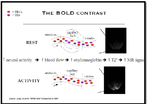
Figure 1- Illustration of the BOLD contrast which measures inhomogeneities in the magnetic field due to changes in the level of O2 in blood. Difference between rest and activity states.

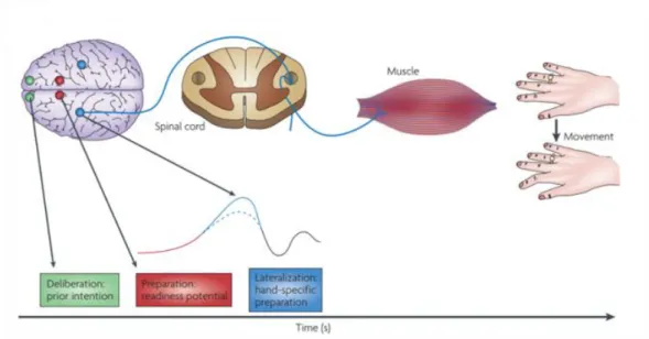
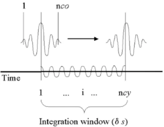
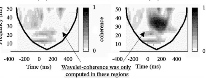
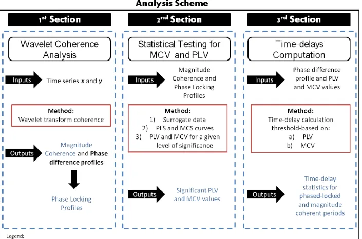
During neural activity there is an increase of blood flow which causes an increase of oxyhemoglobin which is seen in the intensity of MR signal. ... 3 Figure 2- Brain activity preceding a voluntary action of the right hand. The frontopolar cortex (showed in green) forms and deliberates plans and intentions. The pre-SMA (in red) begins the preparation of the action, with other premotor areas, generating the readness potencials, red trace, which can be recorded from scalp. Immediately before the action takes place, M1, (in blue), becomes active. In later stages of preparation the contralateral hemisphere is more active than the ipsilateral hemisphere of the brain (solid and dotted traces). Finally, signal leaves M1 for the spinal cord and to contralateral hand muscles. Addapted from (Haggard 2008). ... 10 Figure 3- Left-hand panel: The primary motor cortex, M1, receives one key input from the supplementary motor area, SMA, and preSMA, which in turn receives inputs from the basal-ganglia and the prefrontal cortex. Right-hand panel: information from early sensory cortices, S1, is relayed to parietal cortex and from there to the lateral part of the premotor cortex, which projects in turn to M1. Adapted from (Haggard 2008). ... 11 Figure 4- Application of the wavelet coherence for two different frequencies. For time and frequency , the Morlet wavelet is defined as the product of a sinusoid at frequency , by a Gaussian window with a standard deviation such that the number of cycles of the wavelet is the same for all frequencies (upper plots, 5 cycles). Since the length of the segments decreases with frequency, it can be seen by comparing (a) and (b) that the length of the integration window decreases with frequency, thus improving the temporal resolution of the coherence estimate. Figure taken from (Lachaux et al. 2002). ... 16 Figure 5- By the convolution of the signal and sucessive nco-cycle Morlet wavelets, the wavelet-coefficients are computed. For each frequency, the wavelet coherence averages the wavelet coefficients over an interval size of that adapts to . corresponds to a constant number of oscillations cycles: . Figure taken from (Lachaux et al. 2002). ... 17 Figure 6- Time-frequency maps for wavelet coherence analysis. On the left: coherence result between two independent signals; on the right: coherence between two signals with a well defined synchronous period. The coherence could not be computed in the regions outside the thick black line because it required data before -400ms or after +600ms outside the recorded interval. Coherence ranges from 0 to 1. Image adapted from (Lachaux et al. 2002). ... 19 Figure 7- Analysis scheme for the three main steps of the presented methodology. The first section is based on Wavelet coherence computation for two chosen time series, x and y. The

(12)

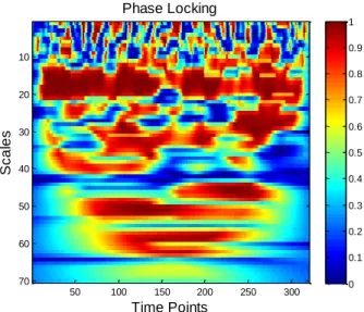
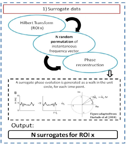
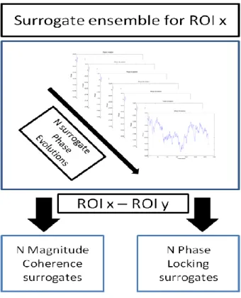
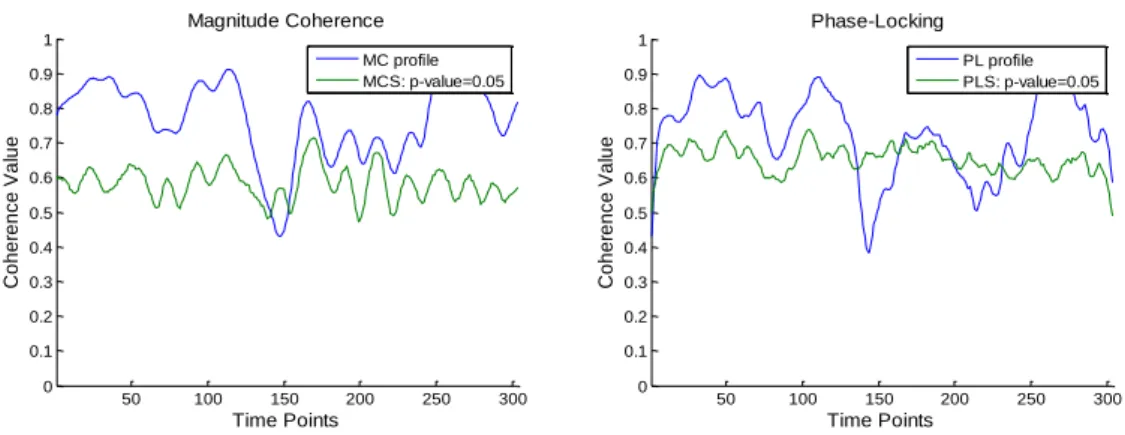
x outputs from this step are both Magnitude Coherence, MC and Phase differences profiles from which the Phase Locking, PL profiles are obtained. On the second section a statistical test is performed for both MCV and PLV using the outputs from the first step as inputs to this section. There is a surrogate data process followed by statistical curves for both PL and MC known as PLS and MCS curves and finally it is applied a statistical decision based on a chosen level of significance to achieve the mentioned outputs. At last, the third section refers to the time-delays computation from the significant statistical PLV and MCV already obtained. Here two different hypothesis of communication are studied , one based on a) PLV and the other on b) MCV as introduced before. The outputs from this analysis are Time-delay statistics for periods of communication between the time series x and y. ... 23 Figure 8- BOLD time courses/time series for two random AAL regions, time series and ,obtained from the pre-processing of data performed on DPARSF toolbox. ... 24 Figure 9- Outputs from WTC function. On the left: matrice for the magnitude coherence values, scaled between [0;1] for both time (time points) and frequency (scales) domains. On the right: matrice for angle difference values, scaled between [ ] for both (time points) and frequency (scales) domains. The values of both magnitude coherence and angle difference are plotted by colormap. ... 24 Figure 10- Phase Locking matrice obtained from Angle difference matrice, Figure 9 on the right, by applying the Phase Coherence integration provided by Lachaux (2002), see equation 6. ... 25 Figure 11- Magnitude Coherence Profile, on the left, and Phase-Locking Profile, on the right - plot of the averaged magnitude coherence/phase locking indexes for a specific narrow frequency band, 0.07-0.13 Hz, and for time points inside influence cone, . ... 26 Figure 12- The surrogate ensemble is performed to a chosen time series named ROI x. It consists on applying the Hilbert Transform to achieve the instantaneous frequencies values from which is made a random permutation N times. This allows one to get a phase reconstrution following Hurtado’ s work. The phase is seen as a walk in the unit circle. From the N random permutation of the power spectrum one gets N surrogates for ROI x. ... 28 Figure 13- Representation of the MCV and PLV procedure. After the computation of the surrogate ensemble for a seed ROI x, it is obtained both N Magnitude Coherence and N Phase-Locking profiles for a ROI pair x and y. ... 29 Figure 14- Phase Locking and Magnitude Coherence Analysis for significant MCV and PLV. In blue: Phase Locking and Magnitude Coherence profiles for a specific pair of ROI signals. In green: PLS and MCS curves for p-value=0.05... 30 Figure 15-A On the left: Magnitude Coherence-based functional connectivity matrix. On the right: Phase-Locking -based functional connectivity matrix. Each matrix entry presents an

(13)

xi averaged value of MC/PL for each ROIs pair for all 116 AAL list of brain regions used on pre-processing (see Appendix 1- AAL brain regions used on DPARSF). ... 33 Figure 16- Brain Mapping for averaged time-delays, in seconds (represented by hot colormap), between a seed region (Left SMA) and a target set of regions. For this example all time-delays have positive values. On the left: brain mapping for communication on significant magnitude coherence periods for 5% level of significance. On the right: brain mapping for communication on significant phase-locked periods for 5% level of significance. The images were obtained overlapping the time-delays values on an anatomical template, MNI template, using the xjview toolbox for MATLAB. ... 34 Figure 17- On the left: Magnitude Coherence profile for Left SMA-Left Insula regions. Blue line: Magnitude Coherence profile for the frequency band 0.07-0.13Hz. Green line: Magnitude Coherence Statistical curve for p-value=0.05. On the Right: Magnitude Coherence profile for Left SMA-Left Insula regions. Blue line: Magnitude Coherence profile for the frequency band 0.07-0.13Hz. Green line: Magnitude Coherence Statistical curve for p-value=0.05. ... 34 Figure 18- On the left: Histogram for time-delays, in seconds; on the right: Histogram for phase-delays, in degrees, for significant Phase-Locking periods. ... 35 Figure 19- On the left: Histogram for time-delays, in seconds; on the right: Histogram for phase-delays, in degrees, for significant Magnitude Coherence periods. ... 36 Figure 20- Values of Mutual Information, ploted with a red color, and values of pearson correlation, ploted with a blue color, for a set of brain regions bellonging to the Parietal-premotor network, PPN. These results correspond to the self-paced finger movement acquisition state. ... 36 Figure 21- Functional Connectivity matrices for all resting states (for subject 1). On the left: functional measure based on Magnitude Coherence metric and on the right: functional measure based on Phase-Locking. From top to bottom: 1st resting state; 2nd resting state; and 3rd resting state moment of the analyzed paradigm. ... 38 Figure 22- Functional Connectivity matrices for action states (for subject 1). On the left: functional measure based on Magnitude Coherence metric and on the right: functional measure based on Phase-Locking metric. From top to bottom: Voluntary action corresponding to self-paced finger movement and Stimulus action corresponding to auditory-self-paced finger movement. ... 39 Figure 23-Functional connectivity sub-matrices focusing the DMN brain regions, presented on Table 4, for subject 1.On the left: Magnitude Coherence metric; on the right: Phase-Locking metric. From top to bottom: 1st resting state; 2nd resting state and 3rd resting state ... 41 Figure 24- Functional connectivity focusing the DMN brain regions presented on Table 4. Left panel: sub-matrices for subject 2; Right panel: sub-matrices for subject 3. For both panels: on

(14)

xii the left: Magnitude Coherence metric; on the right: Phase-Locking metric. From top to bottom: 1st resting state; 2nd resting state and 3rd resting state. ... 42 Figure 25- Functional connectivity focusing FCMN brain regions, presented on Table 4. From top: sub-matrices for subjects 1, 2 and 3, respectively. On the left: Magnitude Coherence metric; on the right: Phase-Locking metrics. ... 43 Figure 26- Functional Connectivity focusing PPN brain regions presented on Table 4. On the left top: sub-matrices for subject 1 during both voluntary and stimulus action and for both MC and PL metrics. On the right top: sub-matrices for subject 2. On bottom: sub-matrices for subject 3. ... 44 Figure 27- Time-delays, in seconds, between Left SMA and PPN regions, for both voluntary and stimulus-driven actions and based on both MC and PL measures of neuronal communication periods. ... 45 Figure 28- Results for L_SMA-L_precentral area during voluntary and stimulus-driven finger movement states. On the left column: Magnitude and Phase-Locking profiles over all time-points; on the middle column: time-delays distribution for both MC and PL measures; on the right column: phase-delays distribution for both MC and PL measures. ... 47 Figure 29- Results for L_SMA-R_precentral area during voluntary and stimulus-driven finger movement states. On the left column: Magnitude and Phase-Locking profiles over all time-points; on the middle column: time-delays distribution for both MC and PL measures; on the right column: phase-delays distribution for both MC and PL measures. ... 48 Figure 30- Results for L_SMA-L_postcentral area during voluntary and stimulus-driven finger movement states. On the left column: Magnitude and Phase-Locking profiles over all time-points; On the middle column: time-delays distribution for both MC and PL measures; On the right column: phase-delays distribution for both MC and PL measures. ... 49 Figure 31- Results for L_SMA-R_postcentral area during voluntary and stimulus-driven finger movement states. On the left column: Magnitude and Phase-Locking profiles over all time-points; on the middle column: time-delays distribution for both MC and PL measures; on the right column: phase-delays distribution for both MC and PL measures. ... 50 Figure 32- ROIs scheme of chronometry-based information flow for brain regions belonging to the FCMN. Each color represents a brain area. Blue circle:Left Basal Ganglia (L_BG); Red:Left SMA(L_SMA) and Green: Left Precentral area. The black arrows show the information flow. On the left: posterior view; in the middle: lateral view and on the right: superior view of the human brain. ... 52 Figure 33- ROIs scheme of chronometry-based information flow for brain regions belonging to the PPN. Each color represents a brain area. Red circle:Left Postcentral; Grey: Left inferior parietal; Pink:Left SMA(L_SMA) and Green: Left Precentral area. The black arrows show the

(15)

xiii information flow chronometry. On the left: posterior view; in the middle: lateral view and on the right: superior view of the human brain. ... 53 Figure 34- Phase distributions for voluntary action (subject 1). On the left column: significant values for MC-based neuronal communication and on the right column: significant values for PL-based neuronal communication PL. From top to bottom: L_SMA-right anterior cingulum; L_SMA-left anterior cingulum; L_SMA-right insula and L_SMA-left insula. ... 57 Figure 35- Phase distributions for voluntary action (subject 2). On the left column: significant values for MC-based neuronal communication and on the right column: significant values for PL-based neuronal communication PL. From top to bottom: L_SMA-right anterior cingulum; L_SMA-left anterior cingulum; L_SMA-right insula and L_SMA-left insula. ... 58 Figure 36- Phase distributions for voluntary action (subject 3). On the left column: significant values for MC-based neuronal communication and on the right column: significant values for PL-based neuronal communication PL. From top to bottom: L_SMA-right anterior cingulum; L_SMA-left anterior cingulum; L_SMA-right insula and L_SMA-left insula. ... 59 Figure 37- Averaged and standard deviation Phase-delays, in seconds units. On the first row: results of subject 1; on the second row: results for subject 2 and the third row presents the results for subject 3. The lef column presents the phase-delays values based on MC measure and the right columns shows the phase-delays values based on PL measure. For each case it is presented the results for Left SMA seed region in relation to Right M1, Left M1, Right PPC and Left PPC. Dark green bar: first resting state moment; green bar: stimulus-driven action (auditory-paced finger movement) and yellow bar: voluntary action (self-paced finger movement). ... 60 Figure 38- Scatter plot, linear regression and linear correlation values, represented by R, for different pairs signals time-delays. Each row refers to a random pair of brain signals. The columns show the results for subject 1, 2 and 3, respectively, from left to right. The units of time-delays are seconds. ... 62 Figure 39- Relationship between MC and PL profiles measured by Pearson correlation and mutual information,MI. The MI values are normalized between [0-1]. Each column presents the results for each subject and the first row reggards to voluntary action, self-paced finger movement, whereas the second one refers to stimulus-driven action, auditory-paced finger movement. The blue bars show the Pearson correlation values whereas the red ones show the MI values for each region belonging to the PPN, see Table 4. ... 63 Figure 40- Relationship between MC and PL profiles measured by Pearson correlation and mutual information,MI. The MI values are normalized between [0-1]. Each column presents the results for each subject and the first row reggards to voluntary action, self-paced finger movement, whereas the second one refers to stimulus-driven action, auditory-paced finger

(16)

xiv movement. The blue bars show the Pearson correlation values whereas the red ones show the MI values for each region belonging to the FCMN, see Table 4. ... 64 Figure 41- Comparison between neuronal synchrony detection based on both Magnitude coehrence and Phase-Locking measures. The black bold curve shows the PLV, phase-locking, profile over time and the other black curve shows the MSC, magnitude coherence profile, between s1 and c2 simulated signals with two specific synchronous intervals. PLS line corresponds to the statistical significant PLV in a 95% level of significance. Image taken from (Lachaux et al. 1999). ... 67 Figure 42- Functional Connectivity matrices for all resting states (for subject 2). On the left: functional measure based on Magnitude Coherence metric and on the right: functional measure based on Phase-Locking. From top to bottom: 1st resting state; 2nd resting state; and 3rd resting state moment of the analyzed paradigm. ... 84 Figure 43- Functional Connectivity matrices for action states (for subject 2). On the left: functional measure based on Magnitude Coherence metric and on the right: functional measure based on Phase-Locking metric. From top to bottom: Voluntary action corresponding to self-paced finger movement and Stimulus action corresponding to auditory-self-paced finger movement. ... 85 Figure 44- Functional Connectivity matrices for all resting states (for subject 3). On the left: functional measure based on Magnitude Coherence metric and on the right: functional measure based on Phase-Locking. From top to bottom: 1st resting state; 2nd resting state; and 3rd resting state moment of the analyzed paradigm. ... 86 Figure 45- Functional Connectivity matrices for action states (for subject 3). On the left: functional measure based on Magnitude Coherence metric and on the right: functional measure based on Phase-Locking metric. From top to bottom: Voluntary action corresponding to self-paced finger movement and Stimulus action corresponding to auditory-self-paced finger movement. ... 87

(17)

xv

LIST OF TABLES

Table 1- Table for inputs parameters values for the application illustration of the presented methodology. ... 32 Table 2- Statistical measures(mean, median and standard deviation) for time-delays (in seconds) for both significant MC and significant PL periods at a p-value=0.05 and number of significant bins. ... 35 Table 3- Narrow frequency bands selected for each subject of A dataset. ... 37 Table 4- Brain regions belonging to the default mode network, the frontal-cognitive motor network and parietal-premotor network; the corresponding AAL region number and the corresponding functional connectivity matrix number. The AAL list of regions is on Appendix 1- AAL brain regions . ... 40 Table 5- Set of bilateral brain regions used on a single-subject analysis for a detailed inspection of neuronal communication. *See Appendix 1- AAL brain regions . ... 46 Table 6- Time-delays statistics for L_SMA-M1/S1 bilateral areas pairs, for both hypothesis of communication: MC-Magnitude Coherence and PL-Phase-Locking measures, and for both voluntarVol, and stimulus-driven,Sti, action states. Averaged, median and std statistics are calculated only for periods, time-points, above MCS and PLS for p-value=0.05. Those periods of communication are quantified and presented as significant bins. ... 51 Table 7- Time-delay statistics (average and std values in seconds units) for all subjects during voluntary finger movement for both MC, magnitude coherence, and PL,phase-locking, measures of neuronal communication. The results are presented for four brain regions belonging to the FCMN , see Figure 32. The ROI pairs are defined by its AAL number, see Appendix 1- AAL brain regions . ... 52 Table 8- Time-delay statistics (average and std values in seconds units) for all subjects during stimulus-driven finger movement for both MC, magnitude coherence, and PL,phase-locking, measures of neuronal communication. The results are presented for brain regions belonging to the PPN, see Figure 33. The ROI pairs are defined byits AAL number, see Appendix 1- AAL brain regions . ... 53 Table 9- Time-delay statistics (average and std values in seconds units) for all subjects during voluntary finger movement for both MC, magnitude coherence, and PL,phase-locking, measures of neuronal communication. The results are presented for brain regions belonging to the PPN, see Figure 33. The ROI pairs are defined by its AAL number, see Appendix 1- AAL brain regions . ... 54 Table 10- Time-delay statistics (average and std values in seconds units) for all subjects during voluntary finger movement for both MC, magnitude coherence, and PL,phase-locking,

(18)

xvi measures of neuronal communication. The results are presented for the pairs: L-SMA/ right and left anterior cingulum and insula brain regions. The ROI pairs are defined by its AAL number, see Appendix 1- AAL brain regions . ... 55 Table 11- Time-delay statistics (average and std values in seconds units) for all subjects during stimulus-driven finger movement for both MC, magnitude coherence, and PL, phase-locking, measures of neuronal communication. The results are presented for the pairs: L-SMA/ right and left anterior insula and Heschl brain regions. The ROI pairs are defined by its AAL number, see Appendix 1- AAL brain regions . ... 56

(19)

xvii

LIST OF ACRONYMS

ACC Anterior Cingulum Cortex

AIC Anterior Insular Cortex

BG Basal-Ganglia

BOLD Blood Oxygen Level Dependent

BP Blood Pressure

CBV Cerebral Blood Volume

DCA Dynamic Connectivity Analysis

DC-EEG Direct-current Electroencephalogram

deoxyHb Deoxyhemoglobin

DMN Default-mode- network

DTI Diffusion Tensor Imaging

EEG Electroencephalogram

fMR Functional Magnetic Resonance

fMRI Functional Magnetic Resonance Imaging

HRF Hemodynamic Response Function

ICN Intrinsic connectivity network

ISF Infra- slow Fluctuations

ISO Infra-slow Oscillations

M1 Primary motor cortex

MC Magnitude Coherence

MCS Magnitude Coherence Statistic

MCV Magnitude Coherence Value

MPF Medial Prefrontal cortex

(20)

xviii oxyHb OxyHemoglobin

PCC Posterior Parietal cortex

PL Phase-Locking

PLS Phase-Locking Statistic

PLV Phase-Locking Value

ROI Region of Interest

RSN Resting State Network

SMA Supplementary Motor Area

(21)

1

1- INTRODUCTION

1.1- Brain Imaging Techniques

Neuroimaging includes the use of different techniques which provide information about both structural and functional imaging without invasive neurosurgery. Nowadays there is a considerable number of safe brain imaging techniques allowing the detection of problems within the human brain and the research of how the human brain works. The investigation of how and where in the brain a cognitive process occurs is performed based on tasks and tests varying the level of demand on the cognitive, sensory or motor capacities of the participant. The performance of a task is correlated with physiological measures in a way to relate functions to areas of the brain. Functional imaging deals with the diagnosis of metabolic diseases and lesions such as Alzheimer's disease, with neurological and cognitive research such as the identification of multiple regions and their temporal relationships associated with the performance of a well designed task and also with brain-computer-interfaces. Some of the most known and used functional neuroimaging techniques are: Electroencephalogram, EEG; Near-Infrared Spectroscopy, NIRS, and functional Magnetic Resonance Imaging, fMRI (Raichle 2003).

1.1.1- EEG, NIRS and fMRI

In a brief description EEG refers to the recording of the electrical activity of the brain (more precisely, post-synaptic potentials), over a period of time, resorting to electrodes that are placed on the subject’s scalp. Time dependent signals such as the EEG can be decomposed into a sum of pure frequency components which allows the exploration of the signal in terms of its power spectrum at each frequency. The EEG spectrum includes frequencies from 0 Hz to the limits of the recording equipment (usually the signal is high-passed filtered above 0.1 Hz). The analysis is typically made below 100Hz because it is the band where most of the power of the EEG signal is contained. Within the range from 0.1Hz to 100Hz the analysis is often made by sub-bands, depending on the application. The most commonly used bands are Delta (0.1 – 3.5 Hz); Theta (4.0- 7.5Hz); Alpha (8.0- 13.0 Hz); Beta (14.0 – 30.0 Hz), and Gamma (30.0 – 100 Hz or above) (Niedermeyer & Lopes da Silva 2005). DC-EEG, direct current-EEG, is adopted for a very slow changing EEG signal. The application of a DC amplifier implies that no low frequencies are omitted and thus it is essential when the signal of interest refers to very slow oscillating neurocortical activity such as signal with frequencies below 1Hz (Saab 2009).

NIRS is a brain imaging technique known as near-infrared spectroscopy based on oxyHemoglobin, oxyHb, and deoxyHemoglobin, deoxyHb, concentrations as an indirect measure of brain activity thanks to the relationship between focal brain activity and regional cerebral blood flow. This neurovascular coupling means that increased activity, that requires

(22)

2 additional metabolic supplies such as oxygen and glucose, is accompanied by local vasodilatation and increased blood flow and oxygenation. This metabolic response known as the hemodynamic response function, HRF, follows neural activity by several seconds. (Gervain et al. 2011)

Nowadays Functional Magnetic Resonance Imaging, fMRI, is a powerful technique which is very popular since it can give high quality visualization of the location of activity in the brain resulting from sensory stimulation or cognitive function. Therefore, it allows the study of how the healthy brain works, how it is affected by diseases and how it recovers after damage, and also how drugs can modulate activity (Strother 2006). So research on fMRI has been undergoing a quite considerable increase.

1.1.2- Hemodynamic BOLD- fMRI Response

Brain activity produces neurological signals that can be monitored and fMRI can be used to measure the hemodynamic response of brain in relation to neural activities. Such measurement is achieved by the detection of changes in blood oxygenation since there is a level dependence between the activation of a brain area and the demand of blood flow. When a specific region of the brain is used, there is an increase of blood flow to that same area. So fMRI research is typical focused on the blood oxygenation level-dependent signal named BOLD signal (Damoiseaux et al. 2006). The BOLD response depends on oxygen uptake, cerebral blood volume, CBV, and cerebral flow velocity. During neural activity there is an increase of blood flow causing an increase of oxyhemoglobin which is detectable with functional magnetic resonance imaging techniques. The magnitude and latency of the hemodynamic responses are affected by changes on neural activity associated (Pfurtscheller et al. 2012). After a sensorial stimulation or even after a mental imagery there is an increase in oxygen and glucose consumption supplied by the vascular system. In the most frequently used form of fMRI, the brain's responses to stimulation or task performance are inferred from the effects of local hemodynamic changes that influence microvascular oxygenation and, thus, measurable levels of MR signal strength. Since arterial blood is essentially oxygenated, this method measures the changes occurring on venous blood oxygenation. The relationship between the blood oxygenation level and the signal strength gives, to this form of functional imaging, the name Blood Oxygenation Level Dependent, BOLD. Using this concept the changes in MR strength are mapped and registered into an anatomical image and can specify the functional response to stimulation or task performance (Mcintyre et al. 2003).

The hemoglobin molecule has magnetic properties that differ depending upon whether it is bound to oxygen or not. The oxygenated hemoglobin (Hb) has no unpaired electron and no magnetic moment (it is diamagnetic). In contrast, deoxyhemoglobin (dHb) has unpaired electron

(23)

3 and magnetic moment (it is paramagnetic). Thus, because blood deoxygenation affects magnetic susceptibility, MR pulses used in fMRI should show more signal for blood with oxygen and less signal for blood deoxygenated. Following Figure 1, during neural activity, there is an increase of blood flow which causes an increase of oxyhemoglobin. Such increase is measured by T2*-weighted MRI (Aizenstein et al. 2004) and it is seen in the intensity of MR signal.

Functional neuroimaging using MRI, based on BOLD contrast, allows the evaluation and identification of brain regions that respond to task-induced activation and are functionally connected to other regions (Chang et al. 2009).

1.1.3- Ongoing slow oscillations

The combination of both electrophysiological and neuroimaging data reveals that mammalian brain dynamics is governed by spontaneous modulations of neuronal activity levels in cortical and sub cortical structures that occur in different frequency bands, 0.01-0.1Hz, 0.1-1 Hz, and <0.01 Hz (Palva & Palva 2012). Fluctuations on the lower frequency range are named slow fluctuations or slow oscillations and represent an interesting property of the brain that has been reported in studies with NIRS, EEG and BOLD fMRI signals. These fluctuations are a prominent feature of the mentioned signals, however, their origin is still not known. According to Pfurtscheller (2012) there are a few possibilities such as the firing of neurons in the reticular formation of the brain stem with a 10 seconds period, or alternatively, neurons may slowly modulate their activity level because of intrinsic excitability changes. Additionally, slow

Figure 1- Illustration of the BOLD contrast which measures inhomogeneities in the magnetic field due to changes in the level of O2 in blood. Difference between rest and activity states. During neural activity there is an increase of blood flow which causes an

(24)

4 systemic fluctuations may also be caused due to the dynamics of cerebral auto-regulation (Pfurtscheller et al. 2012).

The discovery that slow fluctuations in BOLD signals are correlated among specific constellations of brain regions, which constitute intrinsic connectivity networks and define the dynamic architecture of spontaneous brain activity at large, cause a resurgence in interest towards this frequency band (Palva & Palva 2012). It is known that intrinsic activity measured with BOLD fMRI and EEG in the resting brain is organized in multiple highly specific functional networks that fluctuate at frequencies between 0.01 and 0.1 Hz (Fox et al. 2005; Pfurtscheller et al. 2012; Yuan et al. 2013). All the findings on slow oscillations cause an increase of investigation on the respective frequency band and the examination of brain activity is not only made to understand differences between rest and task performance but also to explore the spontaneous brain activity present during resting-state (Biswal et al. 1995). Biswal and colleagues were the first to show that these spontaneous fluctuations were coherent within specific neuro-anatomical systems such as the somato-motor system. Such results were then confirmed and extended to other systems as visual, auditory and language processing networks (Biswal et al. 1995; Greicius et al. 2008).

Over time the human cortical activity has been studied in an intensive way at frequencies ranging from 0.5 Hz to several hundred Hz with EEG. The interpretation of the mechanisms and functions of neuronal events can be done in the context of the ongoing large-scale activity taking into account the full bandwidth of cortical oscillations which includes both very fast and infraslow frequencies. Human cortex may generate infraslow oscillations which are not detectable by conventional EEG because its inferior limit of recording bandwidth of ~0.5 Hz. Vanhatalo et al. used DC-coupled EEG scalp recordings to analyze infraslow oscillations, ISOs, and suggested that such oscillations may represent a slow and cyclic modulation of cortical gross excitability. Previous studies (Gilden et al. 2001) have reported that cortical evoked responses and cognitive performance oscillate at an infraslow rate which supports Vanhatalo et al. to suggest that ISOs are not restricted to sleep states and may rather reflect a continuous oscillatory behavior of wide range of brain functions (Vanhatalo et al. 2004).

Pfurtscheller (2012) hypothesized that these slow oscillations reflect the excitability dynamics of cortical networks. The results suggest that slow oscillations are important in movement and decision making (Pfurtscheller et al. 2012).

1.1.3.1- EEG and NIRS signals recordings

Fluctuations around 0.1Hz in the resting brain were previously found in the EEG (Vanhatalo et al. 2004; Witte et al. 2004) and in both HbO2 and Hb concentrations (Roche-Labarbe et al.

(25)

5 spectroscopy, EEG, BP, blood-pressure, respiration and heart rate in the same study allowed the identification of a short-lasting coupling between prefrontal oxyhemoglobin (HbO2) and central

EEG alpha and/or beta power oscillations in the frequency band 0.07 Hz-0.13 Hz with an approximate 100 seconds of duration (Pfurtscheller, Daly, et al. 2012). Pfurtscheller et al. (2012) also provide support for the idea of Mantini et al. (2007) that resting state networks fluctuate with frequencies between 0.01Hz-0.1Hz.

1.1.3.2- Relation between NIRS and BOLD recordings

NIRS recordings during awake rest have demonstrated slow oscillations with dominance at 0.1Hz (Sasai et al. 2012; Zheng et al. 2010). Both NIRS and fMRI- BOLD signals are based on the detection of hemodynamic response caused by neuronal activity and since ISOs have been discovered in NIRS studies it is also expected that fMRI- BOLD show the same specific feature. There are reports of fMRI-BOLD signal fluctuations on the frequency band 0.01 Hz-0.1 Hz, (Palva & Palva 2012) however, there are no reports referring dominance of 0.1 Hz oscillations.

1.1.4- fMRI confounds

The BOLD contrast does not directly measures the neural activity since it depends on cerebral blood flow, blood volume and oxygenation which are coupled with the ongoing neural processes. There are other physiological processes that can affect the brain`s BOLD response such as the cardiac pulsation and the respiration, which can cause confounding signal fluctuations that are generally considered as physiological noise. (Yuan et al. 2013)

This type of physiological noise translates into non-periodic low frequency fluctuations which overlap with BOLD components. These fluctuations can contribute to a significant variance of BOLD signal. Han Yuan et al. investigated whether the low-frequency fluctuation in physiological noise reflects neuronal activities. The observation of correlation between respiration and electrophysiological recordings suggest that the fluctuation of respiration, that is commonly assumed to be the source of physiological noise in BOLD, may be of neural origin. It is important to note some conclusions of Han Yuan et al. which emphasize that when removing the low-frequency respiratory fluctuation from the BOLD signal, a common substrate of neural activity is also removed and therefore any interpretation requires caution. In contrast if choosing not to remove the respiratory- related low-frequency noise in the BOLD signal, such fluctuation remains a source of confound in fMRI data and the yielded functional connectivity results should also be carefully interpreted. So, unfortunately, slow fluctuation can also be related with physiological noise and not only with neural activity. (Yuan et al. 2013)

1.2- Brain Connectivity

Brain connectivity refers to a pattern of anatomical links, statistical dependencies and causal interactions, between different units within nervous system, from which the terms of

(26)

6 Anatomical, Functional and Effective connectivity arise respectively. Brain connectivity is crucial to elucidate how neurons and neural networks process information and the investigation of connectivity patterns plays a crucial role to determine the functional properties of neurons and neuronal systems. The brain is a complex system whose components organize themselves into dynamic patterns and form networks of interactive components. No single nerve cell can carry out the actions that the human brain is able to perform, however, a large number of nerve cells, linked together into networks inherently provided with dynamic connectivity patterns, make possible all the brain functions such as memory, behavior, thought and consciousness. To understand these integrative functions it is required an understanding of brain networks and the complex dynamic patterns created by them (Sporns 2011).

It seems likely that anatomical variability is one of the sources of functional variability, expressed in neural dynamics and behavioral performance. So, brain connectivity refers to a set of different aspects of brain organization and as it was mentioned before there is a fundamental distinction among structural or anatomical connectivity, effective connectivity and functional connectivity (Sporns 2007).

1.2.1- Types of Connectivity

Anatomical connectivity is related to biophysical processes for the signal transmission. It refers to a network of connections, synaptic connections, which link sets of neurons or neuronal elements and it is usually analyzed with parameters such as synaptic strength or effectiveness. Nowadays diffusion weighted imaging techniques, such as Diffusion Tensor Imaging, DTI, are useful as whole brain in vivo markers of temporal changes in fiber tracts, however, they have insufficient spatial resolution.Effective connectivity describes networks of directional effects of one neural element over another one and so it can be seen as a combination of both anatomical and functional connectivity. It attempts to extract networks of causal influences of one neural element over another (Sporns 2007). Functional connectivity is fundamentally a statistical concept that captures deviations from statistical independence between distributed and often spatially remote neuronal units. It measures dynamic and stochastic characteristics as correlation or covariance, spectral coherence and phase-locking among signals of different brain regions over the cerebral information processing to estimate statistical dependence. It is often calculated among all elements of a system like all brain regions, regardless whether these elements are connected by direct structural links. Functional connectivity is highly dependent on time unlike anatomical connectivity. Statistical patterns between neuronal elements fluctuate on multiple time scales, some as short as tens or hundreds of milliseconds. Functional connectivity can be studied using non-invasive techniques such as electroencephalogram, EEG, near-infrared spectroscopy, NIRS, and functional magnetic resonance, fRMI ( Sporns 2007; Vieira 2011).

(27)

7

1.2.2- BOLD-fMRI based connectivity

Nowadays BOLD-fMRI technique is very commonly used to investigate the functional connectivity of the human brain. The degree of functional connectivity can provide information regarding to the engagement of brain areas during both resting and task performance states.

1.2.2.1- Resting State

Recent neuroimaging studies based on BOLD-fMRI signal have lead to the proposal that rest is characterized by an organized default mode network, formed by specific brain regions, that is modulated or deactivated during specific goal-oriented mental activity. The so called default-mode-network, DMN, includes cingulate cortices, inferior parietal regions and medial prefrontal regions (Fox et al. 2005) and shows strong functional connectivity between those regions. The default mode theory also predicts that engagement between these regions diminishes during cognitive tasks, because of the suppression of the circuit during task execution (Hampson et al.,2006). This resting-state organization is also seen as baseline level of activity characteristic of the human brain which seems to be consistent across different subjects and exhibits significant temporal dynamics (Damoiseaux et al. 2006).

The default mode of brain function hypothesis is readdressed from the perspective of the presence of low-frequency BOLD-fMRI signal changes on the frequency band 0.012–0.1 Hz in the resting brain (Fox et al. 2005; Bluhm et al. 2007). Slow network dynamics characterize neuronal activity also during cognitive tasks (Fox et al. 2005).

Spatial-temporally organized low-frequency fluctuations observed in BOLD-fMRI signal during rest states suggest the existence of underling dynamics networks that emerge spontaneously from intrinsic brain processes (Cabral et al. 2011).

Common networks are quantified in terms of their expected percentage BOLD signal change which provides a measure of the dynamics of the fluctuations. The calculation of the typical amount of variation, in percentage, at each voxel's location of the brain allows the association of coherent networks (Damoiseaux et al. 2006). Previous research reported consistently coherent fluctuations in BOLD fMRI signal within neuroanatomical systems (Biswal et al. 1995; Beckmann et al. 2005). Demoiseaux et al. (2006) reported coherent resting fluctuations in regions involved in motor function, visual processing, executive functioning, auditory processing, memory and also in the default-mode-network, DMN.

1.2.2.2- Task execution

When an attention-demanding cognitive task is taking place there are two possible opposite types of response to be observed. A specific set of frontal and parietal cortical regions routinely exhibit activity increases (Andrew & Pfurtscheller 1996; Cabeza 2000; Corbetta, M & Shulman

(28)

8 2002) whereas a different set of regions, including posterior cingulate, medial and lateral parietal, and medial prefrontal cortex (MPF), routinely exhibit activity decreases (Simpson et al. 2001). As the attention demand of the task is increased the activity in positive regions is further increased whereas activity in negative regions is further decreased (McKiernan et al. 2003). Cognitive tasks can recruit processes of attention and working memory which increase frontal and parietal regions activity (Corbetta, M & Shulman 2002). The repetition of the task can create an episodic memory which can attenuate the decrease of activity. This means that self-referential aspects of a task can modulate the activity intensity. Increased activity is expected in response to attention-demanding cognitive tasks in regions whose function supports task execution and decreased activity in regions supporting unrelated or irrelevant processes (Gusnard & Raichle 2001).

A number of networks has been reported in several studies involving motor cortex, visual cortex and not only regions involved in sensory-related processing but also regions involved in higher cognitive functions have been identified (Biswal et al. 1995). During a task execution there are regions from different networks that seem to activate each other (Damoiseaux et al. 2006).

Functional neuroimaging studies commonly use finger tapping tasks to study the human motor system since its simplicity facilitates the study with both normal control subjects and subjects with neuropathologies affecting the motor system. Finger tapping tasks can vary in the complexity of the tapping and also in the presence or absence of a stimulus which makes it flexible to variations of paradigms. Regarding the presence of a pacing stimulus, the studies usually use visual or auditory regularly paced and repetitive stimulus. A stimulus-paced finger tapping performed in the absence of an external stimulus is internally guided (named self-paced finger tapping). Other variations of finger tapping studies is the performance of a single finger movement, performed by the dominant hand; multi-finger sequence and bimanual movements (Witt et al. 2009).

In Witt (2009), a voxel-wise, coordinate-based meta- analysis was performed on 685 sets of activation foci in Talairach space gathered from 38 published studies employing finger tapping tasks, activation on bilateral sensorimotor cortices, supplementary motor areas (SMA) , left ventral premotor cortex, bilateral inferior parietal cortices, bilateral basal ganglia and bilateral anterior cerebellum. Studies investigating both auditory and visual pacing stimulus have reported different networks of active brain regions without consistency across studies. The variations in the experimental paradigms used and the few specific neural regions analyzed on those studies can justify such inconsistency across studies.

(29)

9

Voluntary action

Voluntary action is one of the most characteristic features of the human brain. Nowadays neuroscience is focused on viewing such actions as a complex set of specific brain processes, rather than a transcendental feature of human nature. To investigate these brain processes, neurocientists apply the classic engineering principle of intervening to control inputs and then measure the outputs. Well-designed studies can provide new insights into the volitional brain. For voluntary actions the stimulus-independence causes difficulties on the experimental study of human volition (Haggard 2008).

To capture the concept of voluntary actions being independent on the stimulus, the most common approaches are not adequate because they use a stimulus as an input to measure the system`s output. The most used experimental solution to this problem, according to Haggard (2013) is to provide a stimulus that only partly determines what the participant should do, in one of three ways: the participant performs a fixed action but chooses "when" to perform it; the participant performs an action at a specific time but chooses the number of repetitions of the actions or the participant chooses whether to perform an action or not.

Another important concept is that a voluntary action is not the same as a reflex action. The first one involves the cerebral cortex whereas the second one is purely spinal. It is known that a voluntary action matures late in individual development whereas a reflex can be present at or before birth (Haggard 2008).

The voluntary action involves two distinct subjective experiences which are the "intention" of performing an action, (the planning of doing something) and the experience of "agency" which is the latest feeling that the action performed as indeed cause an external event (Haggard 2008).

(30)

10 Based on Haggard (2008) during the execution of a voluntary finger movement the frontopolar cortex is responsible for the formation and deliberation of plans and intentions, the pre-SMA begins the preparation of the action with other motor areas and immediately before the action takes place the primary motor cortex, M1, becomes active. Then the signal leaves M1 to the spinal cord and then to the contra lateral hand muscles, as shown on Figure 2. According to the results presented by(Jenkins et al. 2000; Brass & Haggard 2007) it is also expected that regions such as the supplementary motor area, SMA, anterior cingulate cortex, ACC and anterior insular cortex, AIC, are activated during self-initiated movements.

Brain Circuits for Voluntary and Stimulus-driven finger movement

Activity on SMA has been linked to higher motor processing functions such as the initiation of movement, motor planning, motor learning and selection of movement. Activation in the basal ganglia has been associated with the performance of simple repetitive movements. Activity on both SMA and basal ganglia has been preferentially linked to internally generated movements over externally generated movements, however this distinction has not been consistently reported (Cunnington et al. 2002). The premotor cortex has been shown to play an important role in the transformation of sensory information into appropriate motor behavior, especially regarding to sequential movements (Ghuman et al. 2013). The parietal cortex has also been shown to be active during auditory-cued movements (Haggard 2008). Dum (2002) suggested that cortical motor areas show similar preferences for voluntary and for stimulus-driven actions,

Figure 2- Brain activity preceding a voluntary action of the right hand. The frontopolar cortex (showed in green)

forms and deliberates plans and intentions. The pre-SMA (in red) begins the preparation of the action, with other premotor areas, generating the readness potencials, red trace, which can be recorded from scalp. Immediately before the action takes place, M1, (in blue), becomes active. In later stages of preparation the contralateral hemisphere is more active than the ipsilateral hemisphere of the brain (solid and dotted traces). Finally, signal leaves M1 for the spinal cord and to contralateral hand muscles. Addapted from (Haggard 2008).

(31)

11 suggesting that there is a distinction in cortical organization of action (Dum et al. 2002). Several neuroimaging investigations have focused on the comparison between brain activity during manual actions performed as a free will action and performed as a stimulus-dependent action.

The human brain contains different relevant cortical motor circuits converging on the primary motor cortex (M1) responsible for the transmission of motor commands to the spinal cord and muscles. M1 receives two broad classes of inputs which subserve voluntary and stimulus-driven actions, such as the finger movement, see Figure 3. According to Haggard (2008) the studies applied on similar manual action based on external stimulus response and based on voluntary response at a time of the participant choice showed stronger activation on pre-SMA for the volition case than for stimulus-driven action. The role of such brain area on voluntary action is confirmed by recordings of electrodes on the scalp showing an activation occurring 1 s or more before the voluntary movement. The onset readiness potential is seen as the initiation of a cascade of neural activity that spreads from the SMA to M1, causing movement. The pre-SMA belongs to a wider frontal cognitive-motor network, see left-hand panel on Figure 3, which includes the premotor, the cingulate and the frontopolar cortices (Haggard 2008). This network is expected on voluntary action and by contrast the parietal-premotor circuit, see right-hand panel on Figure 3, seems to guide stimulus-driven action, however it has also a contribution to voluntary behavior. Another relevant circuit is the basal ganglia-preSMA which can be more involved on immediate action instead of the parietal-premotor circuit since the basal ganglia-preSMA is more directed to the initiation of action than the parietal-premotor circuit which might arbitrate among alternative action. So the basal ganglia-preSMA has a key

role on voluntary action (Haggard 2008).

Figure 3- Left-hand panel: The primary motor cortex, M1, receives one key input from the supplementary motor

area, SMA, and preSMA, which in turn receives inputs from the basal-ganglia and the prefrontal cortex. Right-hand panel: information from early sensory cortices, S1, is relayed to parietal cortex and from there to the lateral part of the premotor cortex, which projects in turn to M1. Adapted from (Haggard 2008).