Performance analysis of Massive
MIMO receivers
Daniel Filipe Sobral Fernandes
A Dissertation presented in partial fulfillment of the Requirements
for the Degree of
Master in Telecommunications and Computer Engineering
Supervisor
Prof. Dr. Francisco António Bucho Cercas, Full Professor
ISCTE-IUL
Co-Supervisor
Prof. Dr. Rui Miguel Henriques Dias Morgado Dinis, Associate
Professor
FCT-UNL
Resumo
Atualmente, sente-se um aumento exponencial nos dispositivos wireless. De modo a permitir uma boa experiência por parte dos utilizadores é fundamental que a próxima geração de comunicações móveis (5G) assegure fiabilidade nas ligações, uma elevada taxa de transferência de dados e baixa latência.
Uma maneira de elevar a taxa de transferência de dados é utilizar sistemas massive Multiple-Input, Multiple-Output (MIMO), ou seja, sistemas com múlti-plas antenas a emitir e múltimúlti-plas antenas a receber permitindo assim diversidade espacial. Nestes sistemas, para aumentar a bateria dos dispositivos é preferível usar no uplink a modulação Single-Carrier with Frequency-Domain Equalization pois esta modulação reduz a complexidade no emissor transferindo-a para o rece-tor, neste caso na Base Station, onde isso é bastante aceitável.
Esta dissertação estuda o desempenho dos recetores dos sistemas massive MIMO, comparando o desempenho alcançado com o desempenho do Matched Filter Bound (MFB). O recetor Iterative Block Decision-Feedback Equalizer (IB-DFE) apresenta um desempenho muito semelhante ao do MFB no entanto, o algoritmo do receptor inverte matrizes, o que nos sistemas em estudo, onde o tamanho das matrizes é elevado, se reflecte no aumento da complexidade das op-erações associadas. Deste modo, é importante que sejam utilizados recetores de baixa complexidade tal como o Maximal-Ratio Combining (MRC) ou o Equal Gain Combining.
Esta dissertação propõe um recetor simples que combina um recetor IB-DFE com um recetor MRC, criando desde modo um recetor de baixa complexidade e com excelente desempenho.
Palavras-chave: SC-FDE, IB-DFE, Zero Forcing, MRC, EGC, MIMO,
Abstract
We face now an exponential increase in wireless devices and to allow good user ex-perience, it is imperative that the next generation of mobile (5G) communications ensures reliable connections, high data transfer rates and low latency.
One way to increase the data transfer rate is to use massive Multiple-Input, Multiple-Output (MIMO) systems, that is, systems with multiple antennas to emit and multiple antennas to receive thus allowing spatial diversity. In these systems, to increase the battery life of the devices it is preferable to use the Single-Carrier with Frequency-Domain Equalization modulation in the uplink as this modulation reduces the complexity in the emitter, transferring it to the receiver, in this case the Base Staion, where it is quite acceptable.
This dissertation studies the performance of massive MIMO receiver systems, comparing it to the performance achieved with the Matched Filter Bound (MFB). The Iterative Block Decision-Feedback Equalizer (IB-DFE) receiver presents a very similar performance to the MFB, however, the algorithm requires matrix inversions, which in the systems under study, where the size of the matrix is high, implies an increase of the associated operations increases. Thus it is very important that low complexity receivers, such as the Maximal-Ratio Combining (MRC) or Equal Gain Combining are used.
In this dissertation, a simple receiver is proposed combining the IB-DFE re-ceiver with the MRC rere-ceiver, thus creating a low complexity rere-ceiver with excel-lent performance.
Keywords: SC-FDE, IB-DFE, Zero Forcing, MRC, EGC, MIMO, Massive
Acknowledgements
First of all I would like to thank my supervisor, Prof. Dr. Francisco Cercas, for his constant support, guidance, motivation and encouragement during this work. Likewise, I would also like to thank my co-supervisor, Prof. Dr. Rui Dinis, for his motivation, encouragement and willingness to clarify all the scientific doubts encountered throughout the research work.
Secondly, I would like to thank my parents, my sister, my grandparents and all my family for all the support and dedication given over the years. I also want to thank Susan for her contributions with linguistic advices.
This work would have not been possible without the constant support, moti-vation, company and encouragement of my friends Inês, Pedro, Rodrigo, Miriam, João, André and all the other friends and colleagues. My colleagues and friends of the Portuguese Red Cross - Delegation of Setúbal also supported me at this stage. My final thanks go to the undoubted support promoted by Fundação para a Ciência e Tecnologia in the context of research projects PEst-OE / EEI / LA0008 / 2013 and UID / EEA / 50008/2013 - MM5G.
Resumo iii
Abstract v
Acknowledgements vii
List of Figures xi
List of Acronyms xiii
List of Symbols xv
1 Introduction 1
1.1 Motivation and Scope . . . 1
1.2 Objectives . . . 3
1.3 Thesis Organization . . . 3
1.4 Notation and Simulations Aspects . . . 4
2 State of the Art 5 2.1 Evolution to 5G . . . 5
2.2 Block Transmission Techniques . . . 6
2.2.1 Multicarrier versus Single-Carrier modulations . . . 6
2.2.2 OFDM . . . 7
2.2.3 SC-FDE . . . 9
2.2.4 IB-FDE . . . 11
2.3 Multiple-Input, Multiple-Output systems . . . 14
2.3.1 MIMO . . . 14
2.3.2 Massive MIMO . . . 15
3 Receivers for Massive MIMO 17 3.1 IB-DFE for MIMO systems . . . 17
3.2 Zero Forcing . . . 22
3.3 Linear MRC . . . 25
3.4 Linear EGC . . . 26
4 Low complexity receivers for Massive MIMO systems 31 4.1 Iterative MRC . . . 31
4.2 Iterative EGC . . . 35
4.3 Comparison between receivers . . . 38
4.4 The proposed receiver . . . 43
4.5 Results . . . 45
5 Conclusions and Future Work 51 5.1 Conclusions . . . 51
5.2 Future Work . . . 52
Appendices 55
A Publications 57
2.1 OFDM transmission chain. . . 8
2.2 SC-FDE transmission chain. . . 9
2.3 BER performance comparison for SC-FDE with ZF and MMSE equalization. . . 11 2.4 IB-DFE receiver structure. . . 12 2.5 BER performance for an IB-DFE receiver with four iterations. . . . 13 3.1 MIMO system. . . 18 3.2 MIMO IB-DFE receiver structure. . . 19 3.3 BER performance for IB-DFE receiver with P = 2 MTs and R = 6
BSs. . . 20 3.4 BER performance for IB-DFE receiver with P = 60 MTs and R =
180 BSs. . . 21
3.5 BER performance for IB-DFE receiver with P = 60 MTs and R =
360 BSs. . . 21
3.6 BER performance for IB-DFE and ZF receivers with P = 2 MTs and R = 6 BSs. . . 23 3.7 BER performance for IB-DFE and ZF receivers with P = 60 MTs
and R = 180 BSs. . . 24 3.8 BER performance for IB-DFE and ZF receivers with P = 60 MTs
and R = 360 BSs. . . 24 3.9 Massive MIMO receiver and equalization for linear MRC. . . 25 3.10 BER performance for MRC and EGC receivers with P = 2 MTs
and different values of R BSs. . . 27 3.11 BER performance for MRC and EGC receivers with P = 60 MTs
and different values of R BSs. . . 28 3.12 BER performance for MRC and EGC receivers with P = 120 MTs
and different values of R BSs. . . 28 4.1 Massive MIMO receiver and equalization for iterative MRC. . . 32 4.2 BER performance for MRC receiver with P = 2 MTs and R = 6 BSs. 33 4.3 BER performance for MRC receiver with P = 60 MTs and R = 180
BSs. . . 34 4.4 BER performance for MRC receiver with P = 60 MTs and R = 360
BSs. . . 34 4.5 BER performance for EGC receiver with P = 2 MTs and R = 6 BSs. 36
4.6 BER performance for EGC receiver with P = 60 MTs and R = 180 BSs. . . 37 4.7 BER performance for EGC receiver with P = 60 MTs and R = 360
BSs. . . 37 4.8 BER performance for IB-DFE and MRC receivers with P = 60 MTs
and R = 180 BSs. . . 39 4.9 BER performance for IB-DFE and MRC receivers with P = 60 MTs
and R = 360 BSs. . . 39 4.10 BER performance for IB-DFE and EGC receivers with P = 60 MTs
and R = 180 BSs. . . 40 4.11 BER performance for IB-DFE and EGC receivers with P = 60 MTs
and R = 360 BSs. . . 41 4.12 BER performance for MRC and EGC receivers with P = 60 MTs
and R = 180 BSs. . . 42 4.13 BER performance for MRC and EGC receivers with P = 60 MTs
and R = 360 BSs. . . 42 4.14 Proposed receiver. . . 43 4.15 BER performance for the proposed receiver with P = 2 MTs and
R = 6BSs. . . 46
4.16 BER performance for the proposed receiver with P = 60 MTs and
R = 180 BSs. . . 46
4.17 BER performance for the proposed receiver with P = 120 MTs and
R = 360 BSs. . . 47
4.18 BER performance for the proposed receiver with P = 120 MTs and
R = 480 BSs. . . 48
4.19 BER performance for the proposed receiver with P = 60 MTs and
5G 5G
BER Bit Error Rate
BS Base Station
CP Cycle Prefix
DFE Decision-Feedback Equalizer
EGC Equal Gain Combining
FDE Frequency Domain Equalization
FDM Frequency Division Multiplexing
FFT Fast Fourier Transform
FT Fourier Transform
IB-DFE Iterative Block Decision-Feedback Equalizer
IFFT Inverse Fast Fourier Transform
IoT Internet of Things
ISI Inter-Symbol Interference
MC Multicarrier
MFB Matched Filter Bound
MIMO Multiple-Input, Multiple-Output
MMSE Minimum Mean Square Error
mmW millimeter Wave
MRC Maximal-Ratio Combining
OFDM Orthogonal Frequency-Division Multiplexing PMEPR Peak-to-Mean Envelope Power Ratio
QPSK Quaternary Phase Shift Keying
SC Single-Carrier
SC-FDE Single-Carrier with Frequency-Domain Equalization
SINR Signal to Interference-plus-Noise Ratio
SISO Single-Input, Single-Output
SNR Signal-to-Noise Ratio
SVD Singular Value Decomposition
Bk feedback equalizer coefficient for the kth frequency
Bk,p feedback equalizer coefficient for the kth frequency and the pth
user
Eb average bit energy
F sub-carrier separation
Fk feedforward equalizer coefficient for the kth frequency
Fk,p feedforward equalizer coefficient for the kth frequency and the pth
user
Hk overall channel frequency response for the kth frequency
N number of samples/sub-carriers
NG number of guard samples
Nk channel noise for the kth frequency
N o noise power spectral density (unilateral)
P number of users
R number of receiving antennas
R(f ) Fourier transform of r(t)
S(f ) frequency-domain signal
Sk kth frequency-domain data symbol
T duration of the useful part of the block
TB block duration
Ts symbol duration
diagonal matrix with normalization parameter
↵ scale factor associated to the nonlinear operation
A matrix diagonal where elements have absolute value of 1 and phase
identical to the corresponding element of Hk
Uk unitary matrix where left column is singular value of Hk
Vk unitary matrix where right column is singular value of Hk
k error terms matrix for the kth frequency
⌃k matrix diagonal where elements have singular values of Hk
f frequency variable
i iteration index
k frequency index
n time index
p user index
r receiving antenna index
r(t) rectangular impulse; shapping impulse
s(t) time-domain signal
sn nth time-domain data symbol
t time variable
yn nth time-domain received sample
¯
Sk,p "soft decision" for the kth frequency-domain data symbol of the
pth user
¯
sn,p "soft decision" of the nth time-domain data symbol of the pth user
ˆ
Sk "hard decision" for the kth frequency-domain data symbol
ˆ
sn "hard decision" of the nth time-domain data symbol
⇢ correlation coefficient
˜
Sk estimate for the kth frequency-domain data symbol
˜
Sk,p estimate for the kth frequency and the pth user
˜
sn sample estimate for the nth time-domain data symbol
Introduction
1.1 Motivation and Scope
Communication methods have been around for several centuries. The need for hu-manity to communicate at long distances dates almost as back as huhu-manity itself,
with rudimentary methods dating back to that era. Later in the 19th century, the
technological revolution opened the doors to the introduction of new communica-tion methods and allowed Alexander Bell and Elisha Gray to create the first cable telephone in 1876. Since then, the evolution in this area has been remarkable. We are now in the wireless era, where electromagnetism and a simple set of equations known as Maxwell’s equations built the foundation of global wireless communica-tions. With the recent proliferation and evolution of wireless devices and their use, the content consumed by final users is increasing and getting even more complex with the number of users growing exponentially. For this reasons, the telecommu-nications area is in constant innovation and evolution. We are now moving towards
considerable progress: the 5th generation network of mobile communication.
The next generation network of mobile communications is the natural devel-opment of mobile telecommunication standards due to the exponential growth of the wirelesses traffic volume. This growth results, in part, from the demand of entertainment and news in real-time. This will rise exponentially with the advent
of Internet of Things (IoT), where all our gadgets and machines can be connected and will communicate. As we can see, 5G must support diverse specifications like reliability, lower latency and high data rates. Devices should also present low complexity for an increased battery life [1].
A possible solution to achieve the 5G specifications is to use massive MIMO (Multiple-Input, Multiple-Output) systems, where multiple transmitting and re-ceiving antennas are used. This technology uses the base station not only for the uplink (transmission from the Mobile Terminal (MT) to the Base Station (BS)) but also in downlink (transmission from the BS to the MT) with the channel knowledge, so it is possible to offer spatial multiplexing [2]. In this work the major concern is related to the uplink scenario.
Conventional MIMO receivers have a complex hardware implementation re-lated with matrix inversions and a large energy consumption in order to process the received signal [3]. To achieve the objectives of 5G, the massive MIMO schemes can be combined with Single-Carrier with Frequency-Domain Equalization (SC-FDE), as the channels are highly selective in the frequency.
Iterative receivers, such as the Iterative Block Decision-Feedback Equalizer (IB-DFE), have an excellent performance with MIMO [4] but, by increasing the number of transmit antennas, the size of matrixes grows, raising the complexity of matrix inversions. For this reason, the use of this type of receivers and the linear receiver Zero Forcing (ZF) is very limited.
Although receivers that do not require matrix inversions already exist, like the MRC (Maximal-Ratio Combining) and Equal Gain Combining (EGC), the performance of these receivers does not reach the performance of an iterative receiver, although its complexity is much lower.
All the information stated before leads us to a great issue of research which is the main goal of this dissertation: Is it possible to design a receiver with a similiar performance to the iterative receiver while maintaining the complexity of receivers
1.2 Objectives
Throughout this work, the performance of the receivers that do not require matrix inversion will then be studied using theoretical and simulation tools. Then, the obtained results will be analyzed and compared with the existing state of the art published in recent literature. This, in term, will fulfill the challenge the question presented earlier.
Another objective of this work is to develop these receivers so that they can be used in 5G technology.
Finally, the obtained results will be published in international conferences on Telecommunications.
1.3 Thesis Organization
After this first introductory chapter, chapter 2 begins with the evolution of telecom-munication systems up to date, followed by an explanation of block transmission techniques. In this case, the differences between multicarrier and single-carrier modulations are first explained and then a more detailed explanation is given for Orthogonal Frequency-Division Multiplexing (OFDM) modulation and the SC-FDE modulation. In these explanations, the transmission schemes are presented and their differences are highlighted. In the case of the SC-FDE modulation, the IB-DFE receiver and its performance is presented. Finally, the chapter introduces the concept of MIMO and massive MIMO systems.
In chapter 3, the extension of the IB-DFE receiver for massive MIMO systems is presented. In this case, the scenario under study and the receiver scheme are explained. Subsequently, the performance achieved by this receiver for different case studies, where the number of emitting and receiving antennas varies, is pre-sented. The ZF receiver and its performance is also prepre-sented. Finally, the linear version of the low complexity receivers MRC and EGC is explained.
In chapter 4, the low complexity linear receivers presented earlier are again brought to discussion together with the achieved performance, in this case in its iterative version. In this chapter, a comparison is made between all the iterative receivers presented previously. Finally a receiver of low complexity is proposed and analysed that combines two different receivers.
Finally in chapter 5 the conclusions of the work accomplished and the perspec-tives for the future work are highlighted.
1.4 Notation and Simulations Aspects
Throughout this dissertation, the following notation is adopted: bold upper case letters denote matrices or vectors; IN denote the N ⇥ N identity matrix; (·)T, (·)⇤,
(·)H, diag(·) denote the transpose, complex conjugate, hermitian (complex
conju-gate transpose) and diagonal matrices, respectively; [X]n,m denotes the element of
line n and column m of matrix X. E[·] denotes expectation.
In general, upper case letters denote frequency-domain variables and lower case letters denote time-domain variables; ˜(·), ˆ(·) and ¯(·) denote sample estimates, "hard decision" estimate and "soft decision" estimates, respectively.
The performance results presented in this dissertation were obtained by Monte Carlo simulations using the MatLab software environment.
As the accuracy achieved by the Monte Carlo simulations depends on the number of simulated blocks transmitted, the simulations were conducted with data blocks of N = 256 Quaternary Phase Shift Keying (QPSK) symbols per block. Every channel has 100 slots, symbol-spaced, equal-power multipath components.
In all cases it is assumed perfect synchronism between the transmitted blocks associated to the different users and perfect channel estimation.
State of the Art
This chapter deals with literature review of the most important aspects related to the work herein developed. It is divided as follows: Section 2.1 presents the main
reasons for the development of the 5th generation network of mobile
communica-tion. Section 2.2 describes the OFDM and SC-FDE modulations showing their transmission chain diagrams. The IB-DFE concept is also presented in this sec-tion. Finally, section 2.3 presents the theoretical concepts of MIMO and massive MIMO.
2.1 Evolution to 5G
In 1981, in Norway, it was implemented the first communication system (the first generation) that allowed voice transmission using analog modulation. The search for more advanced voice services and the exchange of small messages urged the need to evolve to the second generation, a digital generation. In the 1980s, the third generation began to be planned, which would bring the Internet to the mobile devices of users anywhere. In order to allow users new levels of experience and multi-service capability, the need to move to the fourth generation has arisen [5]. The requirements currently imposed, such as low latency and high bit rates, lead to the concept of 5G. With the passage from the fourth generation to the fifth
generation the spectral efficiency will increase as well as the data rate which may increase up to 1000⇥. According to [6] this increase of 1000⇥ is due to the extreme densification of active nodes, the use of millimeter Wave (mmW) technology, that allows the establishment of wireless connections with a high data transfer [7] and, finally, the use of MIMO.
2.2 Block Transmission Techniques
This section deals with several block transmission techniques. Initially the Single-Carrier (SC) modulation, where the information is transmitted in the time-domain is discussed. Subsequently the modulations where information is transmitted in the frequency-domain are presented: the Multicarrier (MC) modulations.
2.2.1 Multicarrier versus Single-Carrier modulations
In a Single-Carrier modulation the energy associated with each symbol is dis-tributed over the entire bandwidth. In the time-domain, the expression for the complex envelope of a N-symbol burst (N is considered an even value for reasons of simplicity) can be written as:
s(t) =
N 1X n=0
snr(t nTs), (2.1)
where sn is a complex coefficient corresponding to the nth symbol determined
from a certain constellation (e.g., a QPSK constellation), Ts is the symbol
dura-tion and r(t) represents the transmitted impulse. The corresponding expression in the frequency-domain, represented in 2.2 is obtained by applying the Fourier Transform (FT).
S(f ) =F{s(t)} =
N 1X
in which R(f) is the FT of r(t). Thus the transmission band associated to each
symbol sn is the band occupied by R(f).
Multicarrier modulations are characterized by the transmission of information in the frequency-domain according to the following expression:
S(f ) =
N 1X k=0
SkR(f kF ). (2.3)
During the same time interval, T , the N symbols are distributed by N different
sub-carriers. In expression 2.3, F = 1
T represents the spacing between the
sub-carriers and the Sk symbolizes the kth symbol in the frequency-domain. Applying
the inverse FT the following expression is obtained:
s(t) =F 1{S(f)} =
N 1X k=0
Skr(t)ej2⇡kF t. (2.4)
Frequency Division Multiplexing (FDM) is the simplest multicarrier modula-tion where overlapping of sub-carriers does not occur.
In order for the impulses of r(t) to be orthogonal and thus to avoid ISI (Inter-Symbol Interference), the following condition must be met:
Z +1
1
r(t nTs)r⇤(t n0Ts)dt = 0, n6= n0. (2.5)
For the case of multicarrier modulations the expression is analogous to 2.5:
Z +1
1
R(f kF )R⇤(f k0F )df = 0, k 6= k0. (2.6)
2.2.2 OFDM
In the year of 1966, a multicarrier modulation was proposed, the Orthogonal Frequency-Division Multiplexing (OFDM) [8] in which the information is sent through N subcarriers, respecting the principles of orthogonality [9]. The spacing
between them is F 1
TB, where TB is the duration of an OFDM block, which is
revealed in a total available bandwidth of N ⇥ F . This type of modulation allows a higher spectral efficiency to be achieved when compared to FDM, since, due to orthogonality, the spectrum of the subcarriers may overlap [10].
The data is sent in the frequency-domain and has a size N of {Sk; k = 0, 1, . . . , N
1}, a block of N complex symbols, chosen from a selected constellation (e.g., QPSK
constellation). After the data passes through the Inverse Fast Fourier Transform
(IFFT), a Cycle Prefix (CP) of NG samples is added at the beginning of each block
of N IFFT coefficients. This prefix is a cycle extension, in the time domain, of the
OFDM block. The transmitted block is {sn; n = NG, . . . , N 1} with a time
duration of N + NG.
At the receiver end, after the CP is removed and the data block passes the Fast
Fourier Transform (FFT) block, the samples {Yk; k = 0, 1, . . . , N 1}, already in
the frequency-domain, are subjected to Frequency Domain Equalization (FDE).
After the FDE block, the samples, ˜sn, pass through a decision device yielding an
estimated sample ˆsn. The complete transmission chain is represented in Fig. 2.1.
{ Sk} Channel {yn} { Yk} {s~n} {s^n} Transmiter Receiver IFFT Cyclic Prefix
FFT FDE DecisionDevice
Noise
+
2.2.3 SC-FDE
OFDM modulations are vulnerable to transmitter nonlinearities, especially those associated with power amplifiers since the OFDM scenario undergoes large enve-lope fluctuations and a high Peak-to-Mean Enveenve-lope Power Ratio (PMEPR) [11]. Therefore, this type of modulation should be used in downlink communications [12]. Since with SC-FDE modulations, the signals have low envelope fluctuations and the emitters have a high power efficiency, this type of modulation must be used in the MT, that is, in the uplink scenarios. This allows MTs to be cheap and to increase the life of batteries. However, the signals may suffer from high distor-tion which makes the transmission bandwidth larger than the channels’s coherence bandwidth, thus increasing the complexity of the receivers [13].
{ sn} Channel {Yk} { s n} ~ { sn} ^ {S~k} {Fk} FDE Cyclic Prefix Decision Device FFT IFFT Receiver {yn} Noise Transmiter +
Figure 2.2: SC-FDE transmission chain.
In Fig. 2.2 the block transmission chain is represented for this type of modula-tion. The data is transmitted in blocks of N convenient modulated time-domain
symbols {sn; n = 0, . . . , N 1}, where sn is chosen according to a given mapping
rule (e.g., QPSK constellation with Gray mapping). Before the blocks are trans-mitted, a CP is inserted, as explained in the preceding section, resulting in the
following transmitted signal: {sn; n = NG, . . . , N 1}. At the receiver, the CP
is withdrawn from the received data, obtaining the samples {yn; n = 0, . . . , N 1}
in the time-domain. The yn samples then continue through the transmission
{Yk; k = 0, . . . , N 1} where Yk is characterized by the following expression:
Yk = HkSk+ Nk. (2.7)
In equation 2.7, Hk represents the frequency channel response for the kth
subcar-rier and Nk the Gaussian channel noise component, in the frequency-domain, for
that subcarrier. After the equalizer, the frequency-domain samples ˜Sk result in
expression 2.8.
˜
Sk= FkYk. (2.8)
Fk represents the feedforward coefficient of the equalization process and can be
defined according to the criterion ZF (expression 2.9) or Minimum Mean Square Error (MMSE) (expression 2.10).
Fk= 1 HK = H ⇤ k |Hk|2 (2.9) Fk = Hk⇤ 1 SN R +|Hk|2 (2.10) As it is possible to verify, in the case of the equalizer ZF, the channel is com-pletely inverted which can increase the noise in a frequency-selective channel, resulting in a decrease of the Signal-to-Noise Ratio (SNR). This problem can be overcome using the MMSE [14].
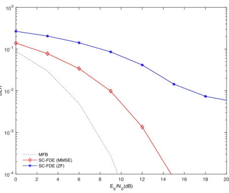
The Bit Error Rate (BER) performance in the scenarios of SC-FDE with ZF and MMSE equalization is presented in Fig. 2.3. In the case of the MMSE criterion, a better performance is achieved due to the fact that this criterion allows to minimize the combined effects of channel noise and ISI.
0 2 4 6 8 10 12 14 16 18 20 E b/N0(dB) 10-4 10-3 10-2 10-1 100 BER MFB SC-FDE (MMSE) SC-FDE (ZF)
Figure 2.3: BER performance comparison for SC-FDE with ZF and MMSE equalization.
2.2.4 IB-FDE
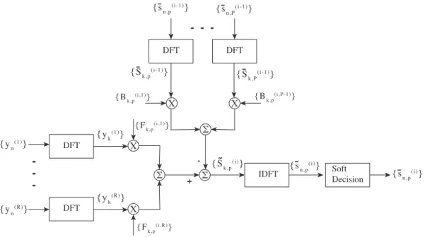
The linear FDE used in both OFDM and SC-FDE schemes allows to achieve good performance. However, to increase the performance of SC-FDE, the linear FDE can be replaced by an IB-DFE, as initially proposed in [15]. This receiver includes two filters: the first one, the feedforward filter, equalizes most of the interference and the second one, the feedback filter, removes some of the residual interference. This is an iterative process that gradually increases the reliability of the received data. Still, this process may not be able to cancel the interference if the first detection is very bad [4]. The structure of this receiver is shown in Fig. 2.4.
In the ith iteration, after the equalizer, the samples in the frequency-domain
are { ˜S(i)
k ; k = 0, 1, . . . , N 1}, with
˜
Sk(i) = Fk(i)Yk Bk(i)Sˆ (i 1)
{ yn} { Yk} {S~k( i)} { S^k( i-1)} {s~n(i)} { s^n(i)} { s^n(i -1)} { Fk ( i )} {Bk (i )} + -DFT IDFT DFT Delay Decision Device
Figure 2.4: IB-DFE receiver structure.
where {F(i)
k ; k = 0, 1, . . . , N 1} is the feedforward coefficient and {B
(i)
k ; k =
0, 1, . . . , N 1} is the feedback coefficient from the Decision-Feedback Equalizer
(DFE) block. The "hard decision" sample from previous iteration is denoted as { ˆSk(i 1); k = 0, 1, . . . , N 1} and represents the DFT of the blocks {ˆs(i 1)n ; n =
0, 1, . . . , N 1} [16].
In order to maximize the Signal to Interference-plus-Noise Ratio (SINR) the feedforward coefficient must be
Fk(i) = H ⇤ k 1 SN R + (1 (⇢(i 1))2)|Hk|2 (2.12) and the feedback coefficients
Bk(i)= ⇢(i 1)(Fk(i)Hk 1), (2.13)
where ⇢ represents the correlation coefficient and is defined by ⇢(i) = E[ ˆS
(i) k Sk⇤]
E[|Sk|2]
. (2.14)
The coefficient of correlation is a parameter that guarantees a good receiver performance because, in the feedback loop, the hard decisions for each block are taken into account, plus the overall reliability of the block, therefore reducing the propagation of errors.
implies B(1)
k = 0and F
(1)
k corresponding to equation 2.10. This happens since there
is no information about snat this time. After this first iteration the coefficient Bk
reduces a large part of residual ISI.
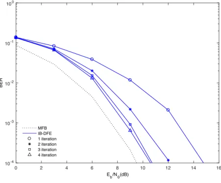
Fig. 2.5 shows the MFB and the BER performance of 4 iterations for the
IB-DFE. As it is possible to verify, in the first iteration, for a value of Eb
N o = 14.7
dB we have a BER = 10 4. For this value of BER over the following iterations
the value of Eb
N o decreases to around 10.5 dB. It is also possible to see that the
performance of iterations 3 and 4 is very similar and both approach the MFB, that is, the simulated samples approach the transmitted samples.
When a pulse is transmitted in an environment without ISI, it is possible to represent the best possible error performance for a receiver, that is, the MFB [17].
0 2 4 6 8 10 12 14 16 Eb/N0(dB) 10-4 10-3 10-2 10-1 100 BER MFB IB-DFE 1 iteration 2 iteration 3 iteration 4 iteration
2.3 Multiple-Input, Multiple-Output systems
In this section the MIMO is initially presented, followed by the massive MIMO.2.3.1 MIMO
In 1996, Foschini [18] demonstrated that multiple streams of data can be transmit-ted at the same frequency by establishing multiple parallel transmission channels. This is only possible if there are several antennas at both the transmitter and the receiver ends. The MIMO systems allow an increase on the reliability of transmis-sion and the coverage area, thus increasing the throughput [19].
This type of MIMO systems undergoes frequency selective fading effects which decrease the performance achieved by the system. In order to minimize this effect, MIMO systems are combined with the OFDM technique. Thus MIMO-OFDM systems transform frequency selective fading into parallel flat fading, where all input signal frequencies suffer the same fading [20, 21, 22].
In order to increase the performance of MIMO-OFDM systems, the Singu-lar Value Decomposition (SVD) linear processing technique can be used. This technique allows the MIMO channel to be decomposed into Input,
Single-Output (SISO) channels and can only be used if the channel matrix (Hk) is known
to the transmitter and the receiver [21].
The SVD of Hk it is given by:
Hk = Uk⌃kVHk , (2.15)
where Uk and Vk are unitary matrices with the columns representing the left
and right singular vector of Hk, respectively. ⌃k is a matrix that in its diagonal
If at the transmitter sn is processed by linear transformation sn = Vsn then
the received signal is:
Yk = HkVkSk+ Nk. (2.16)
By multiplying both elements by UH
k gives:
UHkYk = UHkHkVkSk+ UHkNk. (2.17)
Applying expression 2.15 results in
UkHYk= UHk Uk⌃kVkHVkSk+ UHkNk. (2.18)
As UH
kUk= Iand VHkVk= I, where I represents the identity matrix, equation
2.18 simplifies to
UHkYk = ⌃kSk+ UHkNk. (2.19)
Therefore we conclude that it is possible to treat this system as having SISO channels.
However the main disadvantage of this technique is that the diversity of the signal allowed by the channel is not exploited [13, 21, 23, 24].
2.3.2 Massive MIMO
In order to comply with 5G specifications, there is a need to increase the data rate and to reduce the latency, therefore in [2, 3] the evolution of MIMO, known as massive MIMO, is studied. Massive MIMO systems work with dozens or hundreds of cheap and simple antennas [25]. With this increase of antennas it is possible to direct the energy in a single region, thus increasing the throughput and reducing the power loss.
Since the components are low-power and energy-efficient, it is possible to have devices that consume even less energy.
The existence of flat fading in these systems requires an increase in the trans-mitter power to ensure reliable transmission. As explained in section 2.3.1, it is possible to assume that each channel is only affected by flat fading, using OFDM, which greatly simplifies the analysis. However, and due to the problems presented at the beginning of section 2.2.3, for massive MIMO systems it is preferable to use SC-FDE [13].
Receivers for Massive MIMO
This chapter shows some receivers that can be used in MIMO systems and be extended to massive MIMO systems. The following approach begins with a the-oretical explanation and ends with the presentation of results obtained experi-mentally. Section 3.1 aims to present the extension of SC-FDE with IB-DFE for MIMO systems. In other words, this section will be the extension of section 2.2.4. A linear receiver, which has no iterations, is explained in section 3.2, posteriorly. Subsequently, linear low complexity receivers, MRC and EGC, are presented in sections 3.3 and 3.4, respectively.
3.1 IB-DFE for MIMO systems
In the previous chapter the concept of IB-DFE was associated with a system with an antenna to receive (R= 1) and an antenna to emit (P = 1), i.e., a SISO system.
When passing to a MIMO system [26], with P R, which is shown in Fig. 3.1,
the block diagram shown in Fig. 2.4 may be extended to a block diagram for
detecting the pth MT presented in Fig. 3.2. For the ith iteration, ˜S
k,p (i)
is given by:
˜
MT 1
BS 1
MT P
...
BS R
Figure 3.1: MIMO system.
where F(i)
k,p T
= hFk,p(i,1), . . . , Fk,p(i,R)i and B(i)k,pT = hBk,p(i,1), . . . , B(i,P )k,p i with Fk,p and
Bk,p represent feedforward and feedback coefficients, respectively [27].
Matrix Yk is given by:
Yk =
h
Yk(1), . . . , Yk(R)iT = HkSk+ Nk. (3.2)
This equation (3.2) is analogous to equation 2.8 but in this case it is an
ex-tension for a case with more emitting and receiving antennas. Hk denotes the
R ⇥ P channel matrix for the kth frequency, with (r, p)th element H(r,p)
k , and
Nk=
h
Nk(1), . . . , Nk(R)iT denotes the channel noise.
The DFT of the block in the time-domain {¯s(i)
s,p; n = 0, 1, . . . , N 1}, for
the pth user and for the ith iteration, is the block { ¯S(i)
k,p; k = 0, 1, . . . , N 1}
whose elements constitute the vector ¯S(i 1)
k,p =
h ¯
Sk,1(i), ¯Sk,p 1(i) , ¯Sk,p(i 1), . . . , ¯Sk,P(i 1)iT. The elements ¯sn,p and ¯Sk,p represent the "soft decisions" in the time domain and
frequency domain, respectively. Once the "soft decisions" do "symbol averages" and the "hard decisions" do "blockwise average" [28] the following relationship
{yn (1)} {yk (1)} {Fk,p (i,R)} {yn(R)} {yk (R)} {Fk,p (i,1)} + -{Bk,p(i,1)} {B k,p (i,P-1)} DFT DFT DFT DFT {Sk,p (i-1)} _ {Sk,P (i-1)} _ {s_n,p(i-1)} {s_n,P(i-1)} {S~k,p(i)} IDFT {sn,p (i)} ~ Soft Decision {sn,p (i)} _ . . . . . .
Figure 3.2: MIMO IB-DFE receiver structure.
can be written: ¯ S(i 1)k ' P(i 1)S˜(i)k , (3.3) where P(i 1) = diag(⇢(i 1) 1 , . . . , ⇢ (i 1) P ). (3.4)
The correlation coefficient ⇢(i 1)
P defined in equation 2.14 and ˜S
(i)
k can be
ap-proximated by:
˜
S(i)k ⇡ P(i 1)Sk+ k. (3.5)
In equation 3.5 the coefficient k = [ k,1, . . . , k,P]T has zero mean and it is
uncorrelated with P(i 1). When the first iteration is considered, i = 1, P(0) is a
null matrix which implies that ˜S(0)
k is a null vector [29].
The BER performance of the IB-DFE receiver for a MIMO case, i.e., 2 MTs transmit to 6 BSs (R/P = 3), is shown in Fig. 3.3. As it is possible to verify, the iterations 2, 3 and 4 present very similar performance among themselves and are very close to the MFB, at about 0.4 dB. The first iteration of this receiver to a
0 2 4 6 8 10 12 14 16 E b/N0(dB) 10-4 10-3 10-2 10-1 100 BER MFB IB-DFE 1 iteration 2 iteration 3 iteration 4 iteration
Figure 3.3: BER performance for IB-DFE receiver with P = 2 MTs and R = 6 BSs.
BER = 10 4 has an Eb
N o of approximately 10.3 dB, which is 1 dB higher than the
remaining iterations.
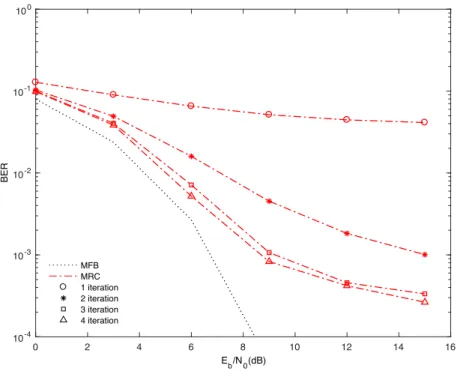
When the use of this receiver is extended to a system with 60 MTs and 180 BSs (R/P = 3), i.e. a massive MIMO system, the performance obtained is shown in Fig.3.4. It is possible to verify that the 4 iterations present the same progress
until they reach an Eb
N o = 6 dB corresponding to a BER ⇡ 10 2. The BER = 10 4
is reached in the first iteration when the Eb
N o = 10 dB and in the fourth iteration
when Eb
N o ⇡ 8.5 dB.
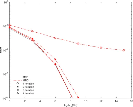
As the R/P increases to 6, as represented in Fig. 3.5, the performance achieved by the receiver is identical to the previous case (Fig. 3.4), so the second, third
and fourth iterations are coincident with each other and reach a BER = 10 4 for
Eb
N o ⇡ 8.4 dB. It can then be verified that the receiver under study presents a
0 2 4 6 8 10 12 14 16 E b/N0(dB) 10-4 10-3 10-2 10-1 100 BER MFB IB-DFE 1 iteration 2 iteration 3 iteration 4 iteration
Figure 3.4: BER performance for IB-DFE receiver with P = 60 MTs and R = 180BSs. 0 2 4 6 8 10 12 14 16 Eb/N0(dB) 10-4 10-3 10-2 10-1 100 BER MFB IB-DFE 1 iteration 2 iteration 3 iteration 4 iteration
Figure 3.5: BER performance for IB-DFE receiver with P = 60 MTs and R = 360BSs.
Despite the excellent performance achieved by this receiver for massive MIMO systems, the algorithm followed presents many matrix manipulations, as previously stated.
Since the complexity of matrix operations depends on their size and once these matrices have very large dimensions, the complexity of the operations makes these receivers not suitable for massive MIMO systems.
3.2 Zero Forcing
In the previous section, an iterative receiver was analyzed that approached the MFB after some iterations. However this type of receiver presents some problems due to its computational complexity. In this section a linear receiver, the Zero Forcing (ZF), is presented.
In this receiver, after the equalizer, the frequency-domain samples ˜Sk are given
by: ˜ Sk = h ˜ Sk(1), . . . , ˜Sk(R)iT = FTkYk= (HkHHk + ↵I) 1HHkYk, (3.6)
where I represents the identity matrix and ↵ = E[|Nk(r)|2]
E[|S(p) k |2]
is assumed identical for all values of r and p [30]. For the receiver under study ↵ = 0 which simplifies the previous equation to:
˜
Sk = (HkHHk ) 1HHkYk. (3.7)
Similarly to the receiver presented in the previous section, this one also presents the necessity of channel inversion for each one of the k frequencies, which makes it too heavy computationally when used for massive MIMO systems.
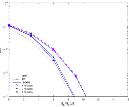
Fig. 3.6 shows the BER performance of the ZF receiver in the case of a MIMO system. Figures 3.7 and 3.8 show the BER performance of the ZF receiver in a massive MIMO system. In these figures, the BER performance for the IB-DFE receiver is also presented because in both systems the BER performance of the ZF
0 2 4 6 8 10 12 14 16 Eb/N0(dB) 10-4 10-3 10-2 10-1 100 BER MFB ZF IB-DFE 1 iteration 2 iteration 4 iteration
Figure 3.6: BER performance for IB-DFE and ZF receivers with P = 2 MTs and R = 6 BSs.
that can be drawn is that for massive MIMO systems the increase of R/P does not modify the performance achieved by this receiver.
As this receiver is not an iterative receiver and its performance is very similar to the first iteration of the IB-DFE, which only differs 1.9 dB from the MFB at
BER = 10 4, this receiver will not be considered in section 4.3, which compares
0 2 4 6 8 10 12 14 16 E b/N0(dB) 10-4 10-3 10-2 10-1 100 BER MFB ZF IB-DFE 1 iteration 2 iteration 4 iteration
Figure 3.7: BER performance for IB-DFE and ZF receivers with P = 60 MTs and R = 180 BSs. 0 2 4 6 8 10 12 14 16 Eb/N0(dB) 10-4 10-3 10-2 10-1 100 BER MFB ZF IB-DFE 1 iteration 2 iteration 4 iteration
Figure 3.8: BER performance for IB-DFE and ZF receivers with P = 60 MTs and R = 360 BSs.
3.3 Linear MRC
As seen in the previous section, IB-DFE receivers present an excellent performance, however, its algorithm includes too many matrix inversions which increases their computational load. For massive MIMO systems, it is fundamental to think of an algorithm that is simpler and does not involve the inversion of matrices such as the Maximal-Ratio Combining (MRC).
Soft Decision IDFT R-branch MRC T size-N IDFTs {Yk} {Sk} ~ {s~n} {s_n}
Figure 3.9: Massive MIMO receiver and equalization for linear MRC.
At the MRC receiver, the signal from each branch is multiplied by a weight factor proportional to the signal amplitude of that branch. So, if a branch presents a weak signal it will be attenuated while a branch with a strong signal will be amplified [31, 32].
The problem of the ZF receiver is related to the channel inversion so, in the case of the MRC, the approximation presented in expression 3.8 simplifies the receiver.
HkHHk ⇡ RI, (3.8)
with I corresponding to the identity matrix. When R 1the correlation between
the channels among different transmit and receive antennas is very small [30]. Thus expression 3.7 of the ZF receiver can be simplified to
˜
S(i)k = HHkYk, (3.9)
where the diagonal of the matrix is represented by and the element (p, p)th is
given by:
N 1XXR
|H(r,p)k |2
! 1
The block diagram of this receiver is shown in Fig. 3.9. Expression 3.10 ensures that the overall frequency response of the "channel plus receiver" for each MT has average 1.
The performance of this linear receiver is represented in figures 3.10, 3.11 and 3.12 together with the receiver performance studied in the next section.
3.4 Linear EGC
In this section we present another low complexity receiver: the Equal Gain Com-bining (EGC).
This receiver does not require channel estimation which makes its implementa-tion simpler when compared to the MRC. In the case of EGC, regardless of signal amplitude of each branch, all branches are weighted by the same factor. In order to avoid the cancellation of the signal, it is necessary to co-phase all the signals [31].
Like in the MRC receiver, when R 1, the small correlation between the
signals from the different emitters and receivers is very small [33]. Thus, the elements outside the diagonal of expression 3.11 are much lower than those of the diagonal.
AHkHk. (3.11)
The elements of the diagonal of A, i.e., the (i, i0)th elements are given by:
[A]i,i0 = exp ⇣
j arg⇣[H]i,i0 ⌘⌘
, (3.12)
so the phase corresponds to the element of matrix H and the absolute value is 1. The receiver and equalization scheme of this receiver is similar to that shown in Fig. 3.9, its only difference being the block corresponding to the "R-branch
At this receiver, the matrix ˜S(i)
k is given by:
˜
S(i)k = HHkYk, (3.13)
Fig. 3.10 shows the performance of linear MRC and EGC receivers in a MIMO system and in figures 3.11 and 3.12 a massive MIMO system is considered. In these figures the number of receiving antennas (R) was varied in order to obtain different R/P values. 0 2 4 6 8 10 12 14 16 Eb/N0(dB) 10-4 10-3 10-2 10-1 100 BER MFB MRC EGC R=4 R=6 R=8 R=10
Figure 3.10: BER performance for MRC and EGC receivers with P = 2 MTs and different values of R BSs.
In the case of the MIMO system (Fig. 3.10), the EGC receiver performs better in comparison to the MRC receiver, however the performance achieved by these receivers is very poor, since the values of BER are too high. It is also possible to verify that with the increase of R/P the performance improves slightly, but even
so the best performance that these receivers present for an Eb
N o = 15 dB is BER
= 8⇥ 10 3 for the case of EGC and a BER ⇡ 10 2, for the case of the MRC with
0 2 4 6 8 10 12 14 16 E b/N0(dB) 10-4 10-3 10-2 10-1 100 BER MFB MRC EGC R=120 R=180 R=240 R=300
Figure 3.11: BER performance for MRC and EGC receivers with P = 60 MTs and different values of R BSs.
0 2 4 6 8 10 12 14 16 Eb/N0(dB) 10-4 10-3 10-2 10-1 100 BER MFB MRC EGC R=240 R=360 R=480 R=600
Figure 3.12: BER performance for MRC and EGC receivers with P = 120 MTs and different values of R BSs.
Considering the massive MIMO system (figures 3.11 and 3.12) the performance achieved with the receivers is similar to the MIMO system. In this type of systems, the MRC receiver achieves better performance than the EGC receiver, and when
R/P = 5, for an Eb
N o = 15 dB, a BER = 1.5 ⇥ 10 2 is reached. It is possible to
verify that when doubling the number of emitting antennas, and maintaining the same R/P relationship, the performance reached by these receivers is very similar.
Low complexity receivers for
Massive MIMO systems
The receivers shown in chapter 3 presented some problems such as their imple-mentation complexity or their poor performance. In this chapter low complexity iterative receivers that can be used in MIMO systems are presented.
This chapter begins with the presentation iteratives versions for the MRC and EGC receivers, in sections 4.1 and 4.2 respectively. In section 4.3 a comparison between the different iterative receivers studied is presented. Finally, in section 4.4 a receiver that tries to overcome the previous drawbacks is proposed.
4.1 Iterative MRC
As shown in the previous chapter, the linear receiver MRC presented a very poor performance and with the increase of R/P it has to take into account the resid-ual interference. Thus, the linear receiver presented previously used iterations to reduce this interference. The iterative MRC receiver is shown in Fig. 4.1 [30] and the corresponding ˜S(i)
k is given by:
˜
S(i) = HH
where B(i)
k reduces interference between users and ISI and is given by:
B(i)k = HHkHk I. (4.2) + -Soft Decision IDFT R-branch MRC T size-N IDFTs T size-N DFTs {Yk} {Sk} ~ {s~n} {s_n} {Sk} _ DFT {Bk}
Figure 4.1: Massive MIMO receiver and equalization for iterative MRC.
Still, in expression 4.1 we have the element ¯S(i)
k =
h ¯
S0(i), . . . , ¯SN 1(i) i that repre-sents the average values, in the frequency domain, conditioned to the FDE output of the previous iteration. This output can be computed as explained in section 3.1.
In the first iteration, i.e. i = 1, there is no previous information ¯S(0)
k = 0, which
causes the receiver to be viewed as a linear MRC. In the following iterations, the results from previous iterations are used to reduce ISI and interference between users.
With the increase on the number of iterations, for moderate-to-high SNR val-ues, the average of the receiver’s output is close to the transmitted signals, which
indicates that the interference cancellation performed by the Bk element becomes
more efficient, leading to an increase in the receiver performance.
In Fig. 4.2 the BER performance of an MRC receiver with 4 iterations for a MIMO system is presented. In the first iteration this receiver has a low slope
dB the curves present the same progress towards the MFB. For higher Eb
N o values
the curves depart from the MFB. In short, this receiver is only efficient for more than 4 iterations. It can also be emphasized that in none of these 4 iterations, the
receiver reaches a BER of 10 4.
0 2 4 6 8 10 12 14 16 Eb/N0(dB) 10-4 10-3 10-2 10-1 100 BER MFB MRC 1 iteration 2 iteration 3 iteration 4 iteration
Figure 4.2: BER performance for MRC receiver with P = 2 MTs and R = 6 BSs.
When the system being studied is a massive MIMO, the performance of the MRC is much better, as shown in figures 4.3 and 4.4. In the case of R/P = 3, shown in Fig. 4.3, and for the first iteration, the performance of the receiver is
quite poor. However the second iteration already reaches a BER = 10 4 when
Eb
N o = 14.4dB, only 6.2 dB apart from the MFB. Iterations 3 and 4 present a very
close performance to the MFB, and for a BER = 10 4 the 3rd iteration already
presents Eb
N o = 8.6 dB and for the 4th iteration
Eb
N o = 8.3 dB that is only 0.03 dB
away from the MFB.
When R/P = 6, as shown in Fig. 4.4, the performance improves reasonably
in comparison with the R/P = 3 case. The first iteration reaches a BER ⇡ 10 2
when Eb
N o = 15 dB and the second iteration for BER = 10
0 2 4 6 8 10 12 14 16 E b/N0(dB) 10-4 10-3 10-2 10-1 100 BER MFB MRC 1 iteration 2 iteration 3 iteration 4 iteration
Figure 4.3: BER performance for MRC receiver with P = 60 MTs and R = 180 BSs. 0 2 4 6 8 10 12 14 16 Eb/N0(dB) 10-4 10-3 10-2 10-1 100 BER MFB MRC 1 iteration 2 iteration 3 iteration 4 iteration
Figure 4.4: BER performance for MRC receiver with P = 60 MTs and R = 360 BSs.
from the MFB, which demonstrates the improvement on the performance with the increase of R/P . The performance achieved with iterations 3 and 4 coincides almost entirely with the performance of MFB.
Therefore, these results show that the performance achieved after only 3 itera-tions is quite good, especially when R/P is substantial, allowing its use in massive MIMO systems.
4.2 Iterative EGC
For MRC receiver, with high R/P , the interference between users and the ISI also increases, so it is important to define a factor that can minimize these effects. This factor, B(i)
k , is given by equation:
B(i)k = AHkHk I. (4.3)
The calculation of ˜S(i)
k is given by [33]:
˜
S(i)k = HHkYk B(i)k S¯(i 1)k . (4.4)
The same assumptions for the MRC receiver can also be taken for the EGC
receiver, that is, for the 1st iteration the receiver can be seen as a linear EGC
receiver and with the increase in the number of iterations its performance increases,
since the cancellation done by matrix Bk becomes more efficient.
The BER performance of the EGC receiver for MIMO systems and massive MIMO systems is shown in figures 4.5, 4.6 and 4.7. It can be verified that for both systems the first iteration is very poor not converging to the MFB. In this case, a performance similar to the MFB performance is also achieved.
For MIMO systems, shown in Fig. 4.5, the second iteration, a BER = 10 4 is
reached when Eb
N o = 14 dB. The performance for the 3
0 2 4 6 8 10 12 14 16 E b/N0(dB) 10-4 10-3 10-2 10-1 100 BER MFB EGC 1 iteration 2 iteration 3 iteration 4 iteration
Figure 4.5: BER performance for EGC receiver with P = 2 MTs and R = 6 BSs.
the same progress as the performance of the MFB over the increase of Eb
N o, however
these curves for a similar value of BER are now separated by about 1.2 dB and 1 dB from the MFB, respectively.
In the case of massive MIMO systems, shown in figures 4.6 and 4.7, the first iteration curve is practically flat. In the case of R/P = 3, Fig. 4.6, the 2nd iteration
never reaches a BER = 10 4. When Eb
N o = 10 dB the 3rd iteration presents a BER
= 10 4 and the performance for the 4th iteration reaches 1.2 dB from the MFB.
With the increase of R/P to 6, Fig. 4.7, the receiver performance improves as
the second iteration reaches a BER = 10 4 for an Eb
N o = 10.5 dB. The 3
rd and 4th
0 2 4 6 8 10 12 14 16 E b/N0(dB) 10-4 10-3 10-2 10-1 100 BER MFB EGC 1 iteration 2 iteration 3 iteration 4 iteration
Figure 4.6: BER performance for EGC receiver with P = 60 MTs and R = 180 BSs. 0 2 4 6 8 10 12 14 16 Eb/N0(dB) 10-4 10-3 10-2 10-1 100 BER MFB EGC 1 iteration 2 iteration 3 iteration 4 iteration
Figure 4.7: BER performance for EGC receiver with P = 60 MTs and R = 360 BSs.
4.3 Comparison between receivers
In this section it is possible to compare the BER performance for the IB-DFE, MRC and EGC receivers. Firstly it is considered a massive MIMO system with
60 MTs and 180 BSs, i.e., R/P = 3 and later on the system considers R/P = 6,
being composed of 60 MTs and 360 BSs.
In figures 4.8 and 4.9 it is possible to compare the first 4 iterations of the
IB-DFE receiver with the MRC receiver. When R/P = 3, Fig. 4.8, the 1st and
2nd iterations of the MRC give bad results, and its performance is worse than
that of the first iteration with IB-DFE. However for a BER = 10 4 the curve for
the fourth iteration of the IB-DFE is 0.5 dB away from the MFB while the 4th
iteration of the MRC coincides with the MFB.
When R/P is increased to 6, Fig. 4.9, the performance of both receivers
improves. Although the 1st iteration of the MRC does not provide good results,
the 2nd iteration provides the performance of the 1st iteration of the IB-DFE. The
performance resulting from the 4th iteration of the MRC coincides with that of
the MFB, and is about 0.2 dB better, than that achieved by the IB-DFE.
It can be concluded that, for a receiver with only one iteration, the IB-DFE receiver is the only technique that achieves the best performance, although pre-senting too much complexity for this type of systems. When the four iterations are considered, the MRC exhibits an excellent performance, which nearly coincides with the MFB, and does not have the complexity of the IB-DFE.
When comparing IB-DFE with the low complexity EGC receiver, as shown in figures 4.10 and 4.11, it is again possible to verify that the first iteration of the low complexity receiver does not give good results, in fact much worse than those of the IB-DFE iterations.
In the case shown in Fig. 4.10, with R/P = 3, the results provided by the 4th
0 2 4 6 8 10 12 14 16 E b/N0(dB) 10-4 10-3 10-2 10-1 100 BER MFB IB-DFE MRC 1 iteration 2 iteration 4 iteration
Figure 4.8: BER performance for IB-DFE and MRC receivers with P = 60 MTs and R = 180 BSs. 0 2 4 6 8 10 12 14 16 Eb/N0(dB) 10-4 10-3 10-2 10-1 100 BER MFB IB-DFE MRC 1 iteration 2 iteration 4 iteration
Figure 4.9: BER performance for IB-DFE and MRC receivers with P = 60 MTs and R = 360 BSs.
of the IB-DFE results in a performance curve that is only 0.3 dB away from the MFB. 0 2 4 6 8 10 12 14 16 Eb/N0(dB) 10-4 10-3 10-2 10-1 100 BER MFB IB-DFE EGC 1 iteration 2 iteration 4 iteration
Figure 4.10: BER performance for IB-DFE and EGC receivers with P = 60 MTs and R = 180 BSs.
When R/P = 6, Fig. 4.11, the 2nd iteration of the EGC provides slightly better
results than the previous case and the 4thiteration results in the performance level
achieved by the 1st iteration of the IB-DFE. The 2nd and 4th iterations lead to
substantially coincident results and for a BER = 10 4 the distance from the MFB
is about 0.2 dB.
In these scenarios, despite the complexity of the IB-DFE, the performance achieved is higher than that of the EGC.
When comparing the two low complexity receivers, as in figures 4.12 and 4.13, it is noticiable that the first two iterations of both receivers lead to very poor
results when R/P = 3, as seen in Fig. 4.12,. While the 4th iteration of the MRC
0 2 4 6 8 10 12 14 16 E b/N0(dB) 10-4 10-3 10-2 10-1 100 BER MFB IB-DFE EGC 1 iteration 2 iteration 4 iteration
Figure 4.11: BER performance for IB-DFE and EGC receivers with P = 60 MTs and R = 360 BSs.
For the case of R/P = 6, Fig. 4.13, the performance of both receivers improve
and the performance resulting from the 2nd iteration of the MRC is better than
that of the 4th iteration of the EGC.
Figures 4.12 and 4.13 show us that the IB-DFE receiver presents a good per-formance as practically all its iterations are close to the MFB. However, it has the disadvantage of being too complex in its implementation for massive MIMO systems.
When considering a receiver of low complexity, like the MRC, and although the first two iterations do not reach a good results, the performance reached after only 4 iterations already coincides with that of the MFB and this is better than the performance achieved by IB-DFE for the same case study.
It can also be concluded that with the increase of R/P the performance of low complexity receivers improves.
0 2 4 6 8 10 12 14 16 E b/N0(dB) 10-4 10-3 10-2 10-1 100 BER MFB MRC EGC 1 iteration 2 iteration 4 iteration
Figure 4.12: BER performance for MRC and EGC receivers with P = 60 MTs and R = 180 BSs. 0 2 4 6 8 10 12 14 16 Eb/N0(dB) 10-4 10-3 10-2 10-1 100 BER MFB MRC EGC 1 iteration 2 iteration 4 iteration
Figure 4.13: BER performance for MRC and EGC receivers with P = 60 MTs and R = 360 BSs.
4.4 The proposed receiver
The simplicity of implementation of the low complexity receivers allows their use in the massive MIMO systems and thus enabling its implementation for the 5G system. However, the performance of these receivers when using only one iteration is very poor. In order to use this receiver for massive MIMO systems it is then necessary to improve the efficiency of the first iteration.
The idea behind the proposed receiver is to improve the effect of the first iteration in order to be able to use low complexity receivers and still achieve a good overall system performance.
The proposed receiver [34] uses the IB-DFE in its first iteration to obtain a good performance and the MRC in the remaining iterations so that the complexity of the receiver allows its use in massive MIMO systems. The proposed receiver scheme is shown in Fig. 4.14.
+ Soft Decision IDFT R-branch MRC T size-N IDFTs 1 iter 1 iter X iter X iter 1st iteration result Remaining iterations results {S~k} {s~n} {s_n} {Yk} {Sk} _ IDFT Soft Decision {s~n} {s_n} {Fk} DFT {Sk} _ {Bk} -T size-N DF-Ts DFT
Figure 4.14: Proposed receiver.
In the first iteration, the proposed receiver behaves as the IB-DFE receiver, so ˜
˜ Sk,p(1) = F(1)k,pTYk B(1)k,p T ¯ S(0)k,p, (4.5) where F(1) k,p T =hFk,p(1,1), . . . , Fk,p(1,R)i and Bk,p(1)T =hBk,p(1,1), . . . , Bk,p(1,P )i with Fk,p(1) = H ⇤ k,p 1 SN R + (1 (⇢(0))2)|Hk,p|2 , (4.6) and Bk,p(1) = ⇢(0)(Fk(1)Hk 1). (4.7)
As in the first iteration, ⇢ = 0 then equations 4.6 and 4.7 can be simplified to
Fk,p(1) = H ⇤ k,p 1 SN R +|Hk,p|2 , (4.8) Bk,p(1) = 0. (4.9) So ˜Sk,p(1) comes ˜ Sk,p(1) = F(1)k,pTYk. (4.10)
Using the IB-DFE in the first iteration, the resulting BER performance is good, as already studied in the previous chapters, however this type of receiver is too complex to be used for the remaining iterations.
Therefore, it is proposed that in the following iterations the receiver uses the
MRC principle, which is a low complexity receiver. So, for these iterations ˜S(i)
k is
where, as presented in section 3.3, represents the diagonal of the matrix
whose element (p, p)th is given by expression 4.12 and the calculation of matrix
B(i)k is represented in equation 4.13.
N 1X k=0 R X r=1 |H(r,p)k |2 ! 1 , (4.12) B(i)k = HHkHk I. (4.13) The ¯S(i)
k element present in expression 4.11 represents the average of the values
resulting from the previous iteration. In the case of the proposed receiver, in the second iteration, this element is the output of the first iteration, that is, the outuput of the IB-DFE receiver. In the remaining iterations that element is derived from the MRC receiver.
4.5 Results
In this section we present the results obtained experimentally for the proposed receiver. In spite of being a receiver designed for massive MIMO systems, the BER performance achieved for a MIMO system is initially presented in Fig. 4.15. The BER performance of the receiver with only one iteration does not match the performance of the MFB, being about 0.7 dB away. With the second and fourth
iterations, values are very similar and the BER = 10 4 is reached for Eb
N o = 9 dB.
After reviewing the performance of the proposed receiver for a MIMO system, the receiver performance for the massive MIMO systems is now analyzed.
In Fig. 4.16 we consider 60 MTs and 180 BSs and in Fig.4.17 120 MTs and
360 BSs are considered, both with R/P = 3. In these two cases the system
performance is quite similar and in the first iteration, for both cases when Eb
N o ⇡ 10
0 2 4 6 8 10 12 14 16 E b/N0(dB) 10-4 10-3 10-2 10-1 100 BER MFB Receiver 1 iteration 2 iteration 4 iteration
Figure 4.15: BER performance for the proposed receiver with P = 2 MTs and R = 6BSs. 0 2 4 6 8 10 12 14 16 Eb/N0(dB) 10-4 10-3 10-2 10-1 100 BER MFB Receiver 1 iteration 2 iteration 4 iteration
Figure 4.16: BER performance for the proposed receiver with P = 60 MTs and R = 180 BSs.
0 2 4 6 8 10 12 14 16 E b/N0(dB) 10-4 10-3 10-2 10-1 100 BER MFB Receiver 1 iteration 2 iteration 4 iteration
Figure 4.17: BER performance for the proposed receiver with P = 120 MTs and R = 360 BSs.
When the second and fourth iterations are applied and for Eb
N o > 6 dB, the
performance practically coincides with that of the MFB. While the MFB reaches
a BER = 10 4 when Eb
N o = 8.24 dB, the proposed receiver, in its fourth iteration,
reaches the same BER performance when Eb
N o = 8.3dB, which , in practical terms,
is equivalent.
These results allow us to conclude that despite the numbers of MTs and BSs may vary, the performance achieved is similar, provided we keep the R/P ratio for a massive MIMO.
In the last two test cases presented we used a R/P = 4, P = 120 and R = 480, as shown in Fig. 4.18 and R/P = 6 (P = 60 and R = 360) as shown in Fig. 4.19. When R/P = 4, it is possible to verify that with the increase of BSs the per-formance is also improved. In this case, the second and fourth iterations give the
same results and from Eb
N o = 6 dB its performance overlaps with the performance
Eb
N o = 9.4 dB and the second iteration of our receiver already coincides with the
MFB performance.
With the increase of R/P to 6, the first iteration of the receiver improves its performance but the following iterations present the same performance achieved for R/P = 4.
It can then be concluded that the proposed receiver performance for massive MIMO systems is excellent since its second iteration coincides with the perfor-mance of the MFB. Besides this excellent perforperfor-mance achieved by the receiver, its level of complexity is kept low, as explained in the previous section.
Another conclusion is that the performance of the proposed receiver improves substantially with the increase of R/P , up to a value of 4.
0 2 4 6 8 10 12 14 16 Eb/N0(dB) 10-4 10-3 10-2 10-1 100 BER MFB Receiver 1 iteration 2 iteration 4 iteration
Figure 4.18: BER performance for the proposed receiver with P = 120 MTs and R = 480 BSs.
0 2 4 6 8 10 12 14 16 E b/N0(dB) 10-4 10-3 10-2 10-1 100 BER MFB Receiver 1 iteration 2 iteration 4 iteration
Figure 4.19: BER performance for the proposed receiver with P = 60 MTs and R = 360 BSs.
Conclusions and Future Work
5.1 Conclusions
The main objective of this dissertation was to analyze the receivers used for massive MIMO systems and to present a solution for a new receiver in the frequency domain that presents low complexity and excellent performance, applicable in the new 5G system.
Initially, in chapter 2, the main differences between multicarrier and single-carrier modulations were presented and it was concluded that in order to reduce the energy expended by the MTs, the SC-FDE modulation should be used in the uplink, since this modulation transfers the complexity of the emitter to the receiver located at the BSs. Also in this chapter the transmission scheme of the iterative receiver IB-DFE was presented and it was verified that its performance approached the MFB. Finally, the MIMO and massive MIMO systems were studied.
In chapter 3, the concept of the IB-DFE receiver was extended to massive MIMO systems together with its performance analysis. It was verified that the performance achieved by MIMO and massive MIMO systems was similar and did not vary with the increase in the R/P ratio. Later on, the linear versions of the ZF, MRC and EGC receivers were presented. In the case of the ZF receiver, the performance achieved was equivalent to the first iteration of the IB-DFE,