Universidade de Lisboa
Instituto Superior de Economia e Gestão - ISEG
ENSAIOS EM ANÁLISE
TÉCNICA E CADEIAS DE
MARKOV
Flavio Ivo Riedlinger de Magalhães
Orientador: Professor Catedrático Doutor João Carlos Henriques da Costa Nicolau Tese especialmente elaborada para obtenção do grau de Doutor em Economia
Esta tese foi financiada pela Fundação para a Ciência e a Tecnologia - FCT SFRH/BD/77426/2011
2018 Júri:
Presidente: Professora Catedrática Doutora Maria do Rosário Lourenço Grossinho Vogais:
Professor Catedrático Doutor António Manuel Pedro Afonso
Professor Catedrático Doutor João Carlos Henriques da Costa Nicolau, Orientador Professor Associado Doutor José Joaquim Dias Curto, Relator
University of Lisboa
Lisboa School of Economics & Management
ESSAYS ON TECHNICAL
ANALYSIS AND MARKOV
CHAINS
Flavio Ivo Riedlinger de Magalhães
Supervisor: Professor Doutor João Carlos Henriques da Costa Nicolau
A thesis submitted in fulfillment of the requirement for the award of the Degree of Doctor of Economics
This thesis was supported by the Science and Technology Foundation - FCT SFRH/BD/77426/2011
2018 Júri:
Presidente: Professora Catedrática Doutora Maria do Rosário Lourenço Grossinho Vogais:
Professor Catedrático Doutor António Manuel Pedro Afonso
Professor Doutor João Carlos Henriques da Costa Nicolau, Orientador Professor Associado Doutor José Joaquim Dias Curto, Relator
Declaration
I certify that except where due acknowledgment is made, this thesis presented to the Lisbon School of Economics and Management (ISEG) in fulfillment of a PhD degree is solely my work. The copyright of this thesis belongs to the author. Quotation from it is permitted, provided that full acknowledgment is made. This thesis may not be reproduced without the prior written consent of the author. I warrant that this authorization does not, to the best of my belief, infringe the rights of any third party. I confirm that in Chapter Four there is a jointly co-authored paper with João Nicolau.
Signature :
Student : Flavio Ivo Riedlinger de Magalhães
To God
Acknowledgment
First and foremost, I want to thank my adviser Professor Catedrático João Carlos Henriques da Costa Nicolau. It has been an honor to be his PhD student. I appreciate all his contri-butions of time and ideas to make my dissertation experience productive and stimulating. Nicolau has given me the freedom to pursue my ideas and provided insightful guidance throughout the writing of the articles bound in this thesis.
I would like to extend thanks to the many people in ISEG who so generously con-tributed to the work presented in this thesis. In particular, special mention and profound gratitude to Alda Soledade Maduro for the support during this challenging years. Alda has been a truly friend. I am also particularly indebted in ISEG to Lurdes da Conceição Ribeiro Rua and my dear PhD colleagues Carla Freire and Hélio Fernandes.
I gratefully acknowledge the PhD fellowship from the Science and Technology Foun-dation (FCT) and the Center for Applied Mathematics and Economics (CEMAPRE). Ad-ditionally, I would like to thank the Instituto Nacional de Matemática Pura e Aplicada (IMPA), for my visiting PhD student experience.
I am deeply grateful to my beloved Raquel for the encouragement and love and to my lovely Valeria and Violeta.
Finally, I must express my very profound gratitude to my family and friends. My unique thanks to my mom for the unconditional love and support in pursuing my dreams. To my dad with love “in memory” and brother Ivo Mauricio. I am also indebted to my friend and tutor, Professor Mario Henrique Simonsen “in memory”. I would like also to extend heartfelt thanks to my very especial friends Luciana Alves, Maria João Correia, Carlos Fagulha, José Alberto Garcia and Maria José Fuertes Guzman for their unconditional support and encouragement. This accomplishment would not be possible without them. Thank you very much.
Abstract
The efficient market hypothesis (Fama, 1970) has been one of the most fundamen-tal pillars of modern financial theory. According to the weak-form of the efficient market hypothesis, prices should reflect all available information. Consequently, it should not be possible to earn excess returns consistently from any investment strategy that attempts to predict asset price movements based on historical data (Fama, 1965; and Fama & Miler, 1972).
Nevertheless, in recent decades, empirical studies have provided evidence that models used for forecasting stock markets, such as technical analysis (TA), which are based on past stock price and volume, can lead to sustainable profitability. Indeed, the TA methodology, which is one of the most widely-used financial market forecasting tools, has been classified as a high-performing method, capable of predicting the stock market.
TA is classified as a price forecasting and market timing methodology, based on the assumptions that markets move in trends, and that these trends persist, suggesting some sort of serial dependency of the behavior of past prices series. In the TA jargon, market action discounts everything.
In this dissertation, we empirically study the predictive power of technical analysis indicators and propose a new theoretical framework, based on a well-defined statistical and mathematical platform. Accordingly, we introduce a new TA methodology, based on multivariate Markov chains. Using as a source the MTD-Probit model proposed by Nicolau (2014), we explore the use of the Markov chain to explain the departure from the martingale property when data snooping is statistically controlled.
Resumo
A hipótese do mercado eficiente (Fama, 1970) tem sido um dos mais fundamentais pilares da teoria financeira moderna. De acordo com a forma fraca da hipótese, os preços dos ativos financeiros devem refletir todas as informações disponíveis. Consequentemente, não é possível obter consistentemente retornos superiores à média do mercado com qualquer estratégia de investimento destinada a prever oscilações dos preços das ações com base em dados históricos (Fama, 1965; e Fama & Miller, 1972).
No entanto, nas últimas décadas, estudos empíricos têm fornecido indícios de que os modelos utilizados para a previsão do mercado de ações com base em informações históricas, como a análise técnica (AT), podem conduzir a uma rentabilidade sustentável. Efetivamente, a metodologia da AT, uma das ferramentas de previsão de mercado financeiro mais ampla-mente utilizada, tem vindo a ser classificada como um método de alta performance, capaz de prever os mercados de ações.
A AT é uma metodologia de previsão de preços e “timing“ de mercado que se baseia nas premissas de que os mercados oscilam por tendências, e de que essas tendências persistem, sugerindo algum tipo de dependência em série com base no seu comportamento passado. No jargão da AT, o mercado desconta tudo.
Nesta dissertação, estudamos empiricamente a capacidade de previsão de indicadores de análise técnica e propomos um novo quadro teórico, baseado numa metodologia estatística e matemática bem definida. Neste sentido, apresentamos uma nova metodologia de AT, com base em cadeias de Markov multivariadas. Utilizando como fonte o modelo MTD-Probit proposto por Nicolau (2014), exploramos o uso da cadeia de Markov para explicar o desvio em relação à propriedade de Martingale quando o ”data-snooping” é estatisticamente controlado.
Contents
Declaration iii Dedication iv Acknowledgment v Abstract vi Resumo viiList of Figures xii
List of Tables xiii
List of Appendices xiv
1 Introduction and Research Overview 1
1.1 Introduction 1
1.2 Research Overview 2
2 Testing the Profitability of Technical Analysis in the PSI-20 Index 4
2.1 Introduction 5
2.2 A Brief Literature Review 6
2.3 The Index, data, and sample selection 7
2.3.1 The PSI-20 7
2.3.2 Data Sample Selection and Descriptive Statistics Results 8
2.4 TA Rules Modeling Framework 10
2.4.1 Technical Indicators Trading Rules 10
2.4.2 TAI Financial Strategy 12
2.4.3 Transaction Costs 13
2.5 Data-Snooping Bias 14
2.5.1 The RC and SPA Tests 15
2.6 Empirical Evaluation 17
2.6.1 Best Performing TAI Trading Rules 17
2.6.1.1 Detailed Technical Analysis Empirical Evidence 18
2.6.2 Robustness Check 23
2.6.2.1 Transaction Costs 25
2.6.2.2 Results of Data-snooping Tests 25
2.7 Conclusion 27
Appendix 1 28
Appendix 2 30
Appendix 3 31
3 The Efficient Market Hypothesis of Stock Prices in the Markov Chain Framework 37
3.1 Introduction 38
3.2 A Brief Literature Review 39
3.3 The Basic Markov Chain Theory 40
3.3.1 First-order Markov Chain 40
3.3.2 High-order Markov Chains 41
3.3.3 The MTD-Probit Estimation Method 42
3.4 The Markov Chain Tests Methodology 44
3.4.1 Introduction 44
3.4.2 The Polansky (2007) Markov chain time-homogeneity Test 45
3.4.2.1 The Polansky Test Method 45
3.4.3 The Anderson and Goodman´s Standard Markov Chain Tests 47
3.4.3.1 The Anderson and Goodman’s time-homogeneity Test 47
3.4.3.2 The Anderson and Goodman’s time-dependency Test 49
3.5 The EMH Test Procedure 50
3.5.1 Introduction 50
3.5.2 The HOMC time-dependence Test Procedure 51
3.5.3 The Polansky time-homogeneity Test Procedure 51
3.5.4 The Anderson and Goodman’s time-homogeneity Test Procedure 53
3.5.5 The State aggregation Method 53
3.6 Empirical Examination 54
3.6.1 Data Sample Selection and Statistics Results 54
3.6.2 Main Sample Index Statistics Results 54
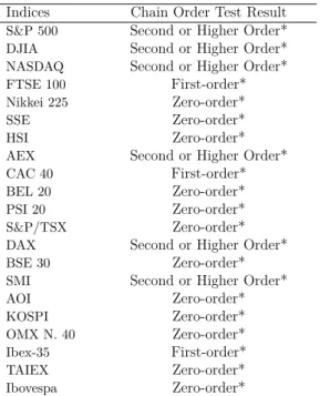
3.6.3 Results of the time-dependence Test 56
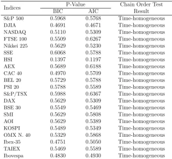
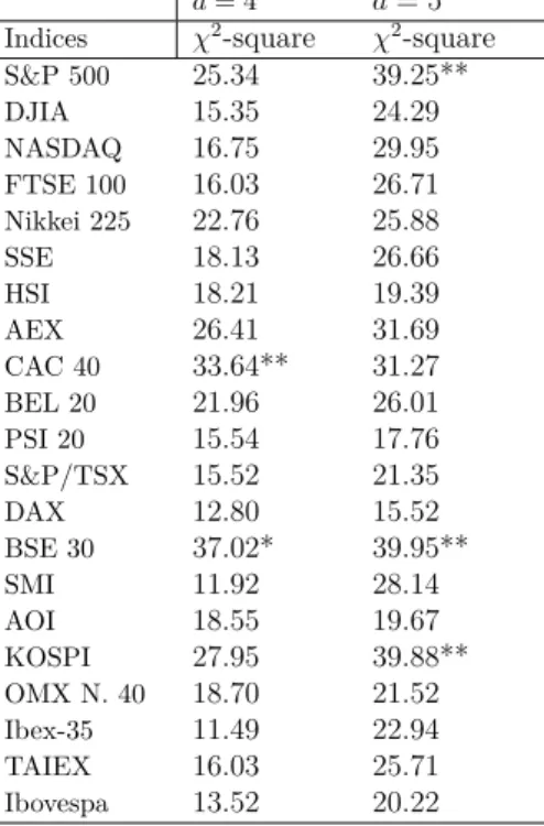
3.6.4 Results of the time-homogeneity Test 59
3.6.5 The Efficient Market Hypothesis 60
3.6.6 A Robustness Results 62
3.7 Conclusions 63
Appendix 1 63
Appendix 2 64
Bibliography 66
4 Estimation and Inference in Multivariate Markov Chains 70 5 The Profitability in the FTSE 100 Index: a New Markov Chain Approach 83
5.1 Introduction 84
5.2 Methodology 85
5.2.1 Multivariate Markov Chain Model and MTD-Probit Estimation Method 85
5.3 Markovian Financial Strategy 87
5.3.1 Modeling Framework 87
5.3.2 The MTD-Probit Forecast Strategy 88
5.3.3 Transaction Costs 90
5.4 Data-Snooping Bias 91
5.4.1 The RC and SPA Tests 91
5.5 Empirical Examination 94
5.5.1 Main Sample Statistics Results 94
5.5.2 Results of the Markovian Stock indices Predictions 95
5.5.3 Robustness Check 98
5.5.3.1 Transaction Costs 99
5.5.3.2 Results of the Data-snooping Tests 99
5.6 Conclusion 100
Appendix 1 101
Appendix 2 101
Bibliography 103
6 The Technical Analysis and the Markov Chain Methodology 108
6.1 Introduction 109
6.2 Technical Analysis and Efficient Market Hypothesis 110
6.3 Methodology 111
6.3.1 The MTD-Probit Estimation Method 111
6.3.2 TA Rules Modeling Framework 113
6.3.2.1 Technical Indicators Trading Rules 113
6.3.3 Noise Reduction Markov Chain Strategy 114
6.3.4 Modeling Framework 115
6.3.5 The MTD-Probit Noise Reduction Forecast Strategy 115
6.3.6 Transaction Costs 118
6.4 Empirical Examination 118
6.4.1 Main Sample Statistics Results 119
6.4.2 Empirical Results 120
6.4.2.1 Best Performing MTD-Probit Trading Rules 120
6.4.2.2 MTD-Probit Noise Reduction Results 121
6.4.2.3 Detailed Empirical Evidence 124
6.4.3 Is the MTD-Probit efficient in noise control? 124
6.5 Conclusion 127 Appendix 1 128 Appendix 2 130 Appendix 3 131 Bibliography 132 7 Conclusion 137
Appendix - Gauss Routines 139
Technical Analysis Routines 140
BBL 140 CCI 140 CHO 141 CMF 142 EMA 143 MACD 144 MFI 144 PPO 145 PVO 146 ROC 147 RSI 147
STO 148 WRI 149 Estimation Routines 151 financial_prediction_MTD_probit 151 matrix_financial_MTDTAI_1 151 matrix_financial_MTDTAI_2 152 matrix_financial_TAI_1 152 matrix_financial_TAI_2 153
Markov Chain Routines 154
categoriza – Nicolau(2014) 154 fv_mul_MC_probit (Nicolau, 2014) 154 MMC_5_log_HOMC 154 MMC_5_probit 155 MMC_5_probit_forecast 156 MMC_5_probit_HOMC 156 multivariate_Markov_Chain_01 (Nicolau, 2014) 157 multivariate_Markov_Chain_02 157 stationary _bootstrap 158 Test Routines 159 mad 159 polansky_homogeneity 159 polansky_time 160 test_bic_aic 160 test_Markov_Chain_Time_Dependence_01 161 test_Markov_Chain_Time_Dependence_12 161 test_Markov_Chain_Time_Homogeneity 162 test__Polansky_bootstrap 162
List of Figures
2.1 PSI - 20 Sample 9
List of Tables
2.1 PSI-20 Composition 8
2.2 PSI-20 Index Returns Descriptive Statistics 9
2.3 TAI Strategies 11
2.4 The Best 10 TAI Trading Strategies Return for the PSI-20 20
2.5 The Best 10 TAI Trading Strategies Return for the PSI-20 21
2.6 The Best 10 TAI Trading Strategies Return for the PSI-20 22
2.7 The Best 10 TAI Trading Strategies Return for the PSI-20 24
2.8 The Best Investment Strategy Data-Snooping Results for the PSI-20 Index 26
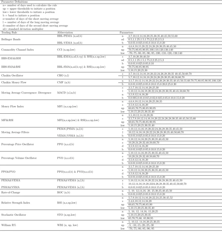
2.9 Technical Analysis Indicators 29
2.10 TAI Parameter Definition 30
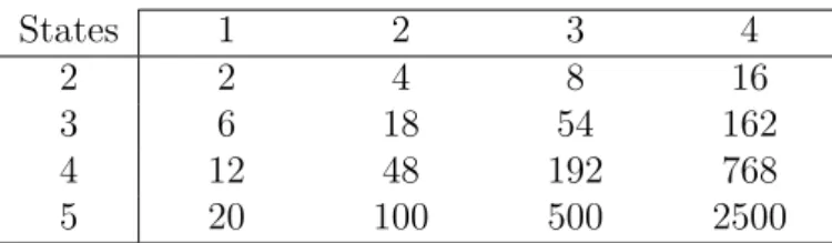
3.1 Number of Parameters for Testing Different Order Markov Chains 50
3.2 Data Sample and Market Capitalization - January, 2015 55
3.3 Indices Descriptive Statistics 57
3.4 Results of the Anderson and Goodman’s Time-dependence Test 58
3.5 Results of the BIC Test for HOMC 58
3.6 Results of the Polanski’s Time-homogeneity Test 59
3.7 Results of the Anderson and Goodman´s Time-homogeneity Test 60
3.8 Results of the Anderson and Goodman’s and Polansky Tests 61
3.9 Results of the Time-Homogeneity and Time-Dependence Tests 62
5.1 FTSE 100 Index Return Descriptive Statistics 95
5.2 The Best 100 Days MTD-Probit Trading Strategies for the FTSE 100 97
5.3 The Best Investment Strategy Data-Snooping Results for the FTSE 100 Index 99
5.4 Explanatory Variables and Parameters MTD-Probit Model 101
6.1 TAI Strategies 114
6.2 FTSE 100 Index Return Descriptive Statistics 120
6.3 The Top 10 Performing MTD-Probit Trading Strategies for the FTSE 100
Index (ODS) 122
6.4 The Best Top 10 MTD-Probit Trading Strategies for the FTSE 100 Index (TRS)123
6.5 The Top 10 Performing Noise Reduction Trading Strategies return for the
FTSE 100 Index (ODS) 125
6.6 The Top 10 Performing Noise Reduction Trading Strategies return for the
FTSE 100 Index (TRS) 126
6.7 Technical Analysis Indicators 129
6.8 TAI Parameter Definition 130
Chapter 1
Introduction and Research Overview
1.1 Introduction
The widespread use of technical analysis (TA) as a leading stock market forecasting tool (see, e.g. Skynkevich, 2012) is still challenging the concept of market efficiency. Since the study of Fama (1970), the efficient market hypothesis (EMH) has been one of the most fundamental pillars in modern finance theory. According to the EMH (Fama, 1965, 1966 and Fama & Miller, 1972), prices should reflect all available information, and it should therefore not be possible to earn excess returns consistently from any investment strategy based on historical data. Consequently, the best conditional choice for future prices should be the current price. That is to say, buying and holding the security is the best investment strategy.
Nevertheless, in recent decades, new empirical evidence has suggested that the stock market can be inefficient, and that it is possible to obtain abnormal stock returns that are not fully explained by common risk measures. In particular, some authors have ad-dressed the possibility that TA could result in sustainable profitability (Murphy, 1986; Sweeney,1986,1988; Brown and Jennings, 1989; Brock et al., 1992; Blume et al.,1994; Neely et al., 1997; Gencay, 1998; Hsu et al., 1999; Lo et al., 2000; Griffioen, 2003; Park and Irwin, 2004 and 2007; Hsu et al., 2010; Neely and Weller, 2011; and Hsu et al., 2013).
The main objective of this dissertation is to study the effectiveness of the technical analysis methodology, and to propose a new multivariate Markov chain (MMC) model to forecast financial market behavior. We believe that the use of this methodology is of special interest in finance, as it is theoretically robust, well defined, and parsimonious. Indeed, the MMC estimation process does not require any extensive set of assumptions, such as the normality distribution, or the existence of homoscedasticity in the series under analysis.
In this context, our key hypothesis is that financial markets are in some way inefficient and that the use of a robust forecasting technique can lead to a substantial profit oppor-tunity. Additionally, we believe that financial time series display a non-random behavior which depends on some independent explanatory variables, and therefore, for forecasting purposes, we have to consider these intrinsic features. This concept is relatively similar to that of the econometrics models which are used to characterize and model financial time series.
In the MMC framework, nevertheless, when the number of categorical data (say s) and the number of states that each financial data can assume (say m) becomes large, any model estimation becomes rapidly intractable, even with moderate values of s and m (e.g. Raftery, 1985 and 1994; Raftery and Tavare, 1994; Berchtold, 1985; Ching et al., 2002 and 2008; and Zhu and Ching, 2010). Nonetheless, a new MMC estimation procedure, called
“MTD-Probit” (Nicolau, 2014), has led to a simpler approach which facilitates model parameter estimation and its statistical inference.
As a result, in this dissertation we forecast the Financial Time-Stock Exchange 100 Share Index (FTSE 100), using a simple trading strategy based on the MTD-Probit estima-tion method. We call this procedure the “markovian MMC indicator” (MMCI). As far as we know, this methodology has never been used to forecast the stock markets.
Furthermore, we carry out inference and model selection, and apply the White (2000) Bootstrap Reality Check (RC) and the Hansen (2005) Superior Predictive Ability (SPA) data-snooping bias tests. These tests allow us to forecast the Index, based on a large set of parameters and co-variables, without any data mining spurious results.
1.2 Research Overview
This dissertation is structured in five interconnected essays, and is divided into two main sections. We follow a “basic focus rationale” and produce a concise study, which could be of innovative interest for the academic and business community alike.
The first section is based on the study of the standard technical analysis framework. Its main focus is to expand our knowledge of the profitability of technical analysis in an unexplored empirical area. In Chapter Two, we therefore propose a study of TA profitability in the Euronext Lisbon stock exchange index, PSI-20.
We analyse the performance of a total of 152,071 trading rules, checking, after con-sidering the costs involved, for the existence of superior returns, compared to adopting the reference strategy, which is buying and retaining the asset (buy-and-hold).
To the best of our knowledge, this is the first paper in which the data snooping con-trolled methodology has been applied in an extensive one-country study of the Portuguese fi-nancial market, which is a relatively “young and less-capitalized” market in a well-developed region.
In the second section, we analyse the previous understanding of the technical analysis methodology and propose a new forecasting instrument, which is dependent on MMC math-ematical framework. The main objective is to provide a sound theoretical structure, based on a well-defined statistical and mathematical platform, which is feasible to be applied in the ”real” world. This section covers four chapters.
In Chapter Three, we explore the standard Markov chains test methodology applied in financial market studies, and propose some reconfiguration to expand its main findings.
In Chapter Four, co-authored with João Nicolau, we closely study the theoretical formulation of the MMC methodology, and thus propose a more structured formulation of the tools used.
Then, in Chapter Five, we introduce a new multivariate Markov chain forecasting methodology based on the MTD-Probit model proposed by Nicolau (2014). We call this procedure the “Markovian MMC indicator”, and use it to forecast the FTSE 100 index.
In Chapter Six, we consolidated all previously discussed concepts, and examine a new research prospect which combines both the Markov chain framework and the standard technical analysis methodology. As a result, we present a new methodology to maximize the performance of any technical analysis trading strategy.
It is well known by financial market professionals that one major difficulty with the use of TA methodology is how to correctly forecast stock price movement signals without being confused by false signals. These trading noises can be seen even in the best-behaved stock price series, and are one of the most challenging problems, as late entries and exit points are responsible for lower investment return.
In this context, we use the MTD-Probit model as a noise control method for the TA strategies, and apply it to forecast the FTSE 100 Index. Our main objective is to provide evidence that this methodology not only potentially controls and filters out false trading signals, but that it is also an important step for the study of TA predictive power.
To the best of our knowledge, this is the first time that Markov chain methodology has been used in conjunction with technical analysis, as part of a stock market investment strategy.
Chapter 2
Testing the Profitability of Technical Analysis in the
PSI-20 Index
Abstract
In this paper, we present a new evidence of the profitability of the technical analysis trading rules in the Portuguese Stock Exchange PSI-20 Index. We apply a total of 152,071 simple and complex trading strategies and test for superior performance compared to the buy-and-hold trading strategy. It has been found that economically significant excess returns over the buy-and-hold trading benchmark strategy are generated, before take in account the effects of data-snooping bias. Nevertheless, the data-snooping tests suggest that the best rule performance across sub-samples is not significant at any significant conventional test level. Indeed, in spite of the wide number of rules tested in this study, our superior profitability could be due to chance rather than to the existence of high-performance strategies. Under such circumstances, the possibility of spurious results is a reasonable assumption.
Keywords: technical analysis, efficient market hypothesis, data-snooping, PSI-20 In-dex.
2.1 Introduction
The efficient market hypothesis (Fama, 1970) has been one of the most fundamental
pillars in modern financial theory. According to the weak-form of the efficient market
hypothesis, prices should reflect all available information; therefore, it should not be possible to earn excess returns consistently with any investment strategy that attempts to predict asset price movements based on historical data (Fama, 1965; and Fama & Miler, 1972).
Nevertheless, in recent decades, empirical studies have provided evidence that models used for forecasting stock markets, based on past stock price and volume, such as technical analysis (TA), can produce sustainable profitability. Indeed, the TA methodology, which is one of the most widely-used financial market forecasting tools (e.g. Shynkevich, 2012), has been considered a high-performance method, capable of predicting the stock market (see among others Sweeney, 1988, and Brock. et al., 1992, Hudson et al., 1996, Taylor, 2000, Skouras, 2001, Park and Irwin, 2004 and 2007, Marshall et al., 2010, Neely and Weller, 2011, and Hsu et al., 2013).
Formally, TA is a price forecasting and market timing methodology, based on the as-sumptions that markets move in trends, and that these trends persist, suggesting some sort of serial dependency about the behavior of past prices series. In the TA jargon, market action discounts everything. Amongst the possible explanations for the superior perfor-mance of TA, is the possibility of a nonlinear stochastic dynamic in stock returns (Berchold and Raftery, 2002), as well as some sort of short-run time inefficiency (Timmermann and Granger, 2004). From this perspective, the TA strategies’ superior profitability could be the result of exploiting those intrinsic characteristics, despite the lack of strong formal mathe-matical and statistical structures.
However, it has been also suggested that the use of TA to forecast financial markets can be profitable only if data-snooping is not statistically controlled. Indeed, it is well known that data-snooping is a typical problem in financial time-series analysis (Lo, 1990, Brock, 1992, White, 2000, Hansen, 2005, Romano and Wolf, 2005, Hsu and Kuan, 2005, Park and Irwin, 2007, Wang, 2007, Romano et al., 2008, Hsu, Hsu, & Kuan, 2010, Park and Irwin, 2010, Day and Lee, 2011, Neuhierl and Schlusche, 2011, Chen et al., 2011, and Yu, 2013).
In this paper, we study the TA profitability in the Euronext Lisbon stock exchange index, the PSI-20. Its main objective is to expand our knowledge of the profitability of technical analysis in an unexplored empirical area. Although there is voluminous literature on the study of the performance of TA, little research has been undertaken to study the Portuguese stock market. Indeed, to the best of our knowledge, this is the first paper in which the data snooping controlled methodology is applied in an extensive one-country study of the Portuguese financial market, which is a relatively “young and less capitalized” market in a well-developed region.
We contribute to the literature in two ways. Firstly, we produce a novel study of the TA rules’ profitability, using a unique broad sample of trading rules. We analyse the performance of a total of 152,071 trading rules, based on well-known mathematically-defined trading rules, checking for the existence of superior returns, after considering the costs
involved, compared to adopting the reference strategy, which is buying and retaining the asset (buy-and-hold). Secondly, we test the TA profitability adjusting accordingly for data-snooping bias, by applying the White (2000) “Bootstrap Reality Check” (RC) and the Hansen (2005) (SPA) tests.
The study shows that before adjusting for data-snooping and transaction costs there is some evidence that TAI rules are capable of consistently producing superior performance over the buy-and-hold benchmark. It was seen that the benchmark is outperformed with an excess return that lies between 43.45% (2011 to 2014) and 14.63% (1993 to 2002). Never-theless, the data-snooping tests suggest that the best rule performance across sub-samples is not significant at any conventional test level. Indeed, in spite of the high number of rules tested in this study, our superior profitability could be due to chance rather than to the existence of high-performance strategies. Thus, we conclude that there is non-significant evidence of abnormal profitability of the TAI strategies applied to forecast the PSI-20, and therefore we cannot rejected the weak-form of the efficient market hypothesis (Fama, 1965 and 1970).
The remainder of this study is organized as follows. The theoretical consideration related to the efficient market hypothesis and technical analysis is presented in Section 2.2. In section 2.3, we present an overview of the PSI-20 Index and define the study sample. In sections 2.4 and 2.5, the trading rules modelling framework and data-snooping test that are used in our study are presented, respectively. In Section 2.6, we present the empirical evaluation of the TA profitability, using controlled data-snooping tests. Finally, Section 2.7 concludes the paper.
2.2 A Brief Literature Review
The use of TA is probably one of the most popular and oldest 1 investment tools among
practitioners, which is used mainly as a complement for fundamental analysis. Indeed, as is acknowledged by Menkhoff (2010) in a survey with 692 fund managers in five countries, TA is a highly used methodology and “is obviously in widespread and of relevant use among fund managers” (p.2573).
However, despite its widespread use, the empirical studies in the area are ambiguous and controversial. On the one hand, there is a body of research that validates the market efficiency and presents contrary evidence for the use of TA as a method that could generate abnormal returns, based on publicly available market information (Fama, 1966; Bessem-binder and Chan, 1995 and 1998; Allen and Karjalainen, 1999; Ready, 2002; Li and Wang, 2007; and Hoffmann and Shefrin, 2014).
On the other hand, several other studies have shown that TA could be a high-performance method capable of analyzing any fundamental stochastic structures presented in financial data series (Sweeney, 1986; Neftci, 1991; Brock et al., 1992; Blume et al., 1994; Sullivan et al., 1999; Lebaron, 1999; Lo et al., 2000; Qi and Wu, 2006; Cheung et al., 2011; Mitra, 2011; Metghalchi et al., 2012; and Shynkevich, 2012).
There are some explanations for these controversial results. We would like to point out two of them. First, the research in this area has proven to be difficult to model, because it re-quires specially-designed forecasting models, as they often exhibit a near-random behavior, which is characterized by non-stationarity, dependence on higher moments, heteroscedastic-ity, and specially, nonlinear behavior (Bollerslev, Chou and Kroner, 1992, Hamilton, 1994, Berchtold and Raftery, 2002, and Gonzalez and Rivera, 2009).
Furthermore, as TA methodology is a highly diverse group of techniques and methods, empirical studies in this area were formulated using several different approaches, ranging from simple trading rules as moving averages, through a complex graphic pattern of analysis recognition 2.
Second, it is considered that the existence of any TA profitable trading rule is just the result of data-snooping. Indeed, it is well known that any empirical result in the financial time-series analysis could produce controversial results, because of the data-snooping bias (e.g. Lo and MacKinlay, 1990, Brock et al., 1992, White, 2000, Hansen, 2005, Lin et al., 2010, Bajgrowicz and Scaillet, 2012, and Kuang et al., 2014).
In this context, the study of technical trading rules’ performance on the Portuguese Stock Exchange is an unexplored empirical area. Indeed, there is only one published global empirical study that examines the predictive-ability of moving average trading rules for 16 European stock markets (Metghalchi et al., 2012), over the 1990 to 2006 period, that included the Portuguese market. Applying the White “Reality Check” (2000) test, the authors presented empirical results that support the superior profitability hypothesis from the technical analysis strategies in the PSI-20 Index.
2.3 The Index, data, and sample selection
In this section, we describe the PSI-20, data and sample selection methodology used in the empirical study of the profitability of TAI rules applied to the PSI-20.
2.3.1 The PSI-20
The PSI-20 Index is the Portuguese stock market index and the benchmark for struc-tured products, funds, exchange traded funds and futures. The Index that was created on 31/12/1992, with a 3,000 points base level, and is a composite of the twenty largest companies in terms of a free float market capitalization. Nowadays, it has a market cap-italization of €41.69 billion (December 31, 2014), and is part of the pan-European stock exchange group, Euronext, alongside Brussels’s BEL20, Paris’s CAC 40, and Amsterdam’s AEX.
Formally, the PSI-20 is a market value-weighted index with a selection principle based 2An extensive review of the use of TA in different scenarios can be found in Park and Irwin (2004) and
on the free float adjusted market capitalization. Companies are selected based on their “velocity threshold” and a minimum “free float” market capitalization of €100 million. The free float is the total of listed shares available for trading, and velocity is the daily ratio of the number of traded and listed shares. The Index composition is annually review in March by an independent PSI Steering Committee. For the annual review, the constituent companies must have an annual trading free float velocity of at least 25% to avoid replacement that can occur quarterly in June, September and December. On January 1, 2014, the Index rules changed. In the new context, the PSI-20 reduced its constituents to a minimum of 18
companies, and lowered the free float market capitalization minimal requirement. Table2.1
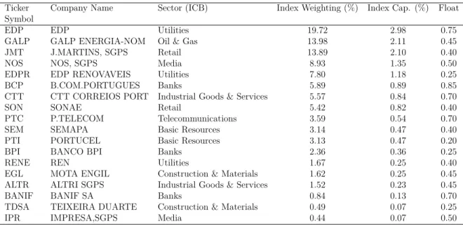
summarizes the PSI-20 composition on December 31, 2014. Table 2.1: PSI-20 Composition
Ticker Symbol
Company Name Sector (ICB) Index Weighting (%) Index Cap. (%) Float
EDP EDP Utilities 19.72 2.98 0.75
GALP GALP ENERGIA-NOM Oil & Gas 13.98 2.11 0.45
JMT J.MARTINS, SGPS Retail 13.89 2.10 0.40
NOS NOS, SGPS Media 8.93 1.35 0.50
EDPR EDP RENOVAVEIS Utilities 7.80 1.18 0.25
BCP B.COM.PORTUGUES Banks 5.89 0.89 0.85
CTT CTT CORREIOS PORT Industrial Goods & Services 5.57 0.84 0.70
SON SONAE Retail 5.42 0.82 0.40
PTC P.TELECOM Telecommunications 3.59 0.54 0.70
SEM SEMAPA Basic Resources 3.14 0.47 0.40
PTI PORTUCEL Basic Resources 3.13 0.47 0.20
BPI BANCO BPI Banks 2.36 0.36 0.25
RENE REN Utilities 1.67 0.25 0.40
EGL MOTA ENGIL Construction & Materials 1.62 0.25 0.45 ALTR ALTRI SGPS Industrial Goods & Services 1.52 0.23 0.45
BANIF BANIF SA Banks 0.84 0.13 0.70
TDSA TEIXEIRA DUARTE Construction & Materials 0.49 0.07 0.25
IPR IMPRESA,SGPS Media 0.44 0.07 0.50
Data Source: Euronext Lisbon, December 31, 2014
2.3.2 Data Sample Selection and Descriptive Statistics Results
In this study, we consider a large Index data sample from January 01, 1993 to December
31, 2014, obtained from the Datastream database. In Table 2.2, we report a summary of
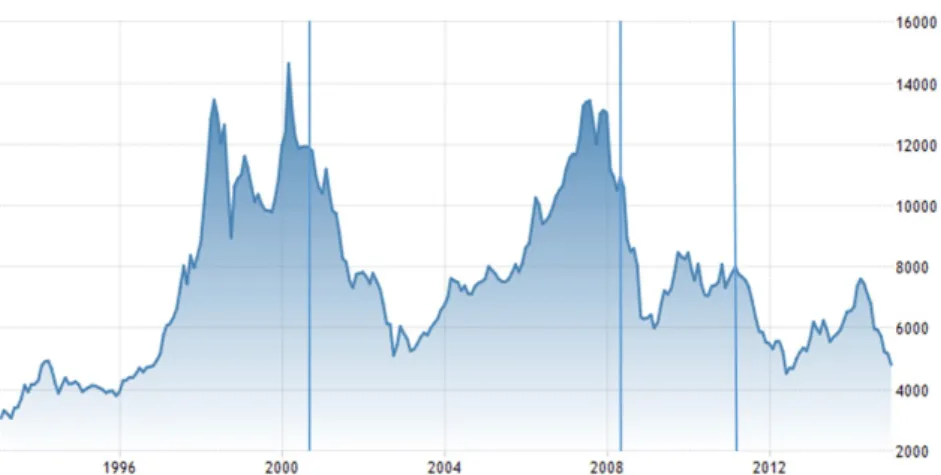
the descriptive statistics for the daily log returns on the indices considered in the paper. We conduct our study on four subsequent sub-samples, in order to provide a dynamic analysis of trading rules performance (e.g. Sullivan et al., 1999, and Park and Heaton, 2014). We consider these sub-samples based on two combined criteria: a time-frame large enough to produce consistent parameter estimation, and some important historical facts that might generate some PSI-20 structural breaks.
In this framework, we selected the first sub-sample based on Portugal’s entrance to
the Euro zone in 20023. We believe that the Euro provoked a permanent effect on the
Index, since it reduced its exchange rate exposure. The second sub-sample corresponds to the sub-prime crisis period in 2008, when major worldwide financial institutions collapsed. The third sub-sample is defined by the European Union financial assistance package signed in May, 2011. Finally, the last period ends in 2014.
Table 2.2: PSI-20 Index Returns Descriptive Statistics
Period 01/01/1993 31/12/2014 01/01/1993 31/12/2001 01/01/2002 30/08/2008 01/09/2008 31/04/2011 01/05/2011 31/12/2014 N(Obs.) 5552 2229 1699 682 939
Mean Daily (%) 8.46E-03 0.043 5.79E-03 -0.0171 -0.0506 Max. (%) 14.6161 12.0992 4.8244 10.1959 5.4612 Min. (%) -12.0992 -14.6161 -6.0125 -10.3792 -4.2669 SD 1.1789 1.1635 0.8777 1.5971 1.3252 Skewness -0.4539 -0.9048 -0.5545 0.1825 -0.3211 Kurtosis 15.8468 24.6197 7.7458 11.5300 3.8445 ρ(1) 0.089* 0.112* 0.054** 0.045 0.121* ρ(2) -0.001* -0.009* 0.044** -0.056 0.030* ρ(3) 0.009* 0.036* 0.059* -0.043 -0.033* ρ(4) 0.037* 0.079* 0.020* 0.054 -0.049* ρ(5) -0.015* 0.023* 0.002* -0.072* -0.041* ρ(6) -0.024* -0.012* -0.034* -0.078** 0.020* Q(6) 56.81* 46.26* 17.03* 14.58** 19.88* JB 38370.12* 43714.83* 1505.22* 2076.24* 44.04*
Notes: Mean Daily (%) is the mean sample log-return, SD is the standard deviation, JB are the Jarque-Bera test statistics, ρ(n) is the estimated auto-correlation at lag n for each series and Q(n) are the Ljung-Box-Pierce test statistics for the nth lag. *
**Statistical Significance at the 10% level for a two-tailed test. **Statistical Significance at the 5% level.*Statistical Significance at the 1% level.
Figure2.1 shows the Index behavior for the entire sample period and sub-samples.
In general terms, our data sample series can be considered consistent for most financial
series distributions. Indeed, as can be seen in Table2.2, the highest mean daily buy-and-hold
return for the PSI 20 Index is 0.043%, which equates to 250 trading days per year, a yearly average of 10.75%. Additionally, the table also shows that the Index is skewed to the left, which indicates that extreme negative returns are more probable than extreme positive ones. The sample excess kurtosis level reveals that the return series has fatter tails than the normal distribution, i.e. low positive and negative returns are more probable. The results show that the first sub-sample (1993-2001) is the highest leptokurtic (24.61) and skewed (-0.9048) period, and that the last sub-sample (2011-2014) has the lowest kurtosis (3.84) and negative asymmetry (-0.3211). There is also evidence of some significant autoregressive process in the PSI-20 return dynamics for some sub-samples, which is a common phenomenon in stock indices returns series. Nevertheless, this linear time dependence can also reflect the existence of a certain level of linear predictability in the index return.
Finally, the Ljung-Box Q statistics rejects, at the 1% level, the null hypothesis of no autocorrelations in the first six lags for the Index and, based on the Jaque-bera test results, the null hypothesis of normality is also rejected.
2.4 TA Rules Modeling Framework
The main goal of this paper is to evaluate TA profitability performance to predict stock market behavior. In this context, it is crucial to select an appropriate set of technical rules since this is an essential step to ensure properly tested procedures. Therefore, in this paper we adopt three basic rules selection criteria: (1) relevance of the instrument; we chose the most widely tools used in the financial market and in the academic literature; (2) replication capacity; we considered only mathematically well-formulated rules, and (3) analytical appropriateness; we selected the rules that are by construction “Markovian times”, as proposed by Neftci (1991). In this scenario, we choose to study technical indicators trading (TAI) rules.
2.4.1 Technical Indicators Trading Rules
In the TA methodology there are special kinds of rules based not on the subjective judgment of figures or chart patterns analysis. Instead, they are focused on market variables data transformation such as trade price, volume and volatility, which can easily be quantified and tested (Murphy, 1986). These strategies can be seen as mathematically well-defined methods for foreseeing securities, based only on the past behavior. Indeed, in the case of these rules, study of historical data is enough to identify some aspects of price dynamics that can produce buy or sell signals, which can be used not only to foresee future changes in prices, but also to provide the information needed to create or adjust any taken market strategy adopted.
In this paper we consider an extensive set of TAI rules, drawn from a wide variety of parametrization specifications that are presented in previous academic studies and also
the technical analysis manuals (see e.g. Edwards and Magee, 2012, and Pring, 2012). As acknowledged by Sullivan et al.(1999), the list of trading rules should be “vastly larger than those compiled in previous studies, and we include the most important types of trading rules that can be parsimonious parametrized and that do not rely on "subjective" judgments” (p.1655).
In this context, we choose a broad set of starting parameters that are presented in the financial literature, such as the number of days of the different horizons time measures, the size of the increase or decrease necessary to generate a buy or sell signal, the number of days’ rate of change in price or volume and overbought/oversold levels. We selected a parameter set that is diversified enough to avoid the type of “survivorship bias” problem related to the best performing historical rules (Sullivan et al., 1999).
Furthermore, since one of the trickiest aspects in technical analysis is the inaccuracy created by short-run false signals we combine TAI strategies, using some complex strategies to confirm an initial trading signal. We want to study multi-indicator trading rules that could help minimize the trading of signal-to-noise and increase profitability (Hsu et al., 2010). We provide an analysis of four complex trading rules. We test the MFI&RSI (Yen and Hsu, 2010), PPO&PVO, PMA&VMA and BBS&RSI. The list of trading rules is presented
in Table 2.3 and in Appendices 1 and 2, we comprehensively detail how the rules and
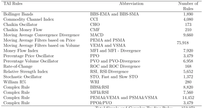
parameter values used in our analysis were defined. As a result, we select a total of 152,071 TAI trading rules parametrization, based on 36 different sets of simple and complex double-rules, provided by the practitioners and academic mainstream literature in the area (see e.g. Brock et al., 1992, and White, 2000).
Table 2.3: TAI Strategies
TAI Rules Abbreviation Number of
Rules
Bollinger Bands BBS-EMA and BBS-SMA 1,890
Commodity Channel Index CCI 4,080
Chaikin Oscillator CHO 173
Chaikin Money Flow CMF 210
Moving Average Convergence Divergence MACD 9,660
Moving Average Filters based on Price PEMA and PSMA
75,918 Moving Average Filters based on Volume VEMA and VSMA
Money Flow Index MFI and MFI - Divergence 7,920
Percentage Price Oscillator PPO 3,479
Percentage Volume Oscillator PVO and PVO-Divergence 6,958
Rate-of-Change ROC and ROC Divergence 168
Relative Strength Index RSI, RSI-Divergence 5,652
Stochastic Oscillator STO, Fast and Slow STO 1,372
William R% WRI 280
Complex Rule BBS&RSI 8,820
Complex Rule MFI&RSI 7,560
Complex Rule PEMA&VEMA and PSMA&VSMA 14,452
Complex Rule PPO&PVO 3,479
2.4.2 TAI Financial Strategy
This section presents our trading rule methodology used to forecast the PSI-20 Index. We assume the existence of some sort of serial dependency on prices that can be seen as a generalization of McQueen and Thorley´s (1991) approach for analyzing stock returns pre-dictability.
We propose evaluating a market strategy using a very simple approach. We assume that the investor buys or sells the PSI-20 Index, according to the trading signal based on the TAI estimation model.
We study the proposed strategy under two different investor behavior assumptions: the one-day strategy (ODS) and the trend reversal strategy (TRS). In the first strategy, we assume the naive and costly hypothesis that any signal lasts for a one-day period only. In the second strategy, we consider that the investor liquidates the position, only if it has a trend reversal signal, for example, from a buy signal to a sell signal.
To sum up, the procedure can be described through the following algorithm:
Step 1: For each sub-sample, we split our dataset into two segments. Then, we use the first t observations to determine the first TAI signals for buy, sell or no action, where the sell signal implies short selling. The size of t is given by the minimum size that is needed to calculate all the TAI trading rules.
Although it is not possible to sell short owing to legal or market restrictions, we follow the approach that it is essential to accurately calculate a total trading rule profitability. Additionally, if our investment rule indicates a no-change market (no action) we account for no return 4.
Step 2: We use the t + 1 observations to re-value the next TAI signals, and so on, sequentially, until we reach a time horizon of n predictions trading signals.
Step 3: We record all the returns that our trading rules are generating and measure total net returns. Mathematically, the returns are determined based on the signal function for the kth TAI rule, k = 1, ..., M , given by:
R∗k,t= Rk,t− R0t, (2.1)
Rk,t = Ik,tRt− abs(Ik,t− Ik,t−1)T c, (2.2)
Rt = ln(pt/pt−1), (2.3)
where Rk,t∗ is the one-day excess return of the kth TAI strategy discounting the market
benchmark strategy R0
t, which in our case is the buy-and-hold trading strategy, after
ac-counting for the one-way transaction cost T c. Furthermore, pt is the daily closing quote of
the index at time t and Ik,t is a variable indicator for the kth TAI rule, which takes the
values 1,0 or -1, respectively if we take a long, no action or short position in t, respectively. Step 4: For each model set up, we calculate the percentage success rate (PSR), based on the predictive accuracy of the trading signals generated in the previous steps, as follows:
P SRk= Vk/n, (2.4)
where Vk is the number of times that our kth TAI trading model estimated signal matches
the real market movement in our forecasting horizon.
Step 5: We evaluate the performance of our forecast methodology, using the White (2000) “Bootstrap Reality Check” and the Hansen (2005) data-snooping test. More details of the bootstrap method and tests applied in this study are presented in Section 5.
2.4.3 Transaction Costs
In this study, we do not consider transaction costs directly, but make a simple assumption that T c = 0. There is no doubt that an investment rule is profitable only when its profit is greater than any trading costs. However, the recent introduction of a new computational trading floor process and online trading systems have lowered the overall “transactional costs” (see e.g. Bessembinder and Chan, 1995, Mitra, 2010, Bajgrowicz and Scaillet, 2012, and Kuang et al., 2014). Therefore, it is very difficult to choose any previous or recom-mended one-way transaction costs level.
To minimize the effects of this “somewhat unrealistic assumption” (Bajgrowicz and Scaillet, 2012), we present a break-even transaction costs analysis based on the method-ologies of Hsu et al. (2010) and Mitra (2010). Then, we calculate the “potential margins for profitability” (PMP) that is the level of T c which could offset any foreseen profitability. As proposed the PMP is the break-even transaction cost, which measures the trading rule capacity to absorb any transaction costs (see e.g. Hsu et al., 2016). It is estimated as follows:
P M P = RT k
Nk
, (2.5)
where RT kand Nk are respectively, the total return and the number changing signals
gener-ated along the investment period horizon for the kth TAI rule. In our investment method-ology, the transaction cost depends of the type of market strategy adopted. In the case of ODS, it is payable twice in each investment decision (round-trip cost), that is:
Nk= n
X
t=1
2 ∗ abs(Ik,t). (2.6)
However, in the TRS case, the transaction cost should be considered initially when a buy/sell signal generates an investment position, and secondly, when a new signal is generated; requiring a change in the previous investment decision as follows:
Nk= n X t=1 abs(Ik,t− Ik,t−1). (2.7)
2.5 Data-Snooping Bias
Many authors have raised concerns about reusing the same data set to test model forecasting accuracy, as this could generate a data-snooping bias (Lo, 1990, Brock, 1992, Hsu and Kuan, 1999, White, 2000, Hansen, 2005, Hsu and Kuan, 2005, Romano et al., 2005, Park and Irwin, 2010, Day and Lee, 2011, Neuhierl and Schlusche, 2011, Chen et al., 2011, and Yu, 2013). Indeed, the possibility of spurious results is a reasonable assumption since superior profitability could be due to chance rather than to the existence of high-performance strategies.
Two different approaches are described in the literature to overcome such biases. The first approach is to validate the forecasting results based on an available comparable data set or in out-of-sample testing (see, e.g. Lo and MacKinlay, 1990). However, such a procedure is not only dependent on existence of a comparable data set, but it is also highly sensitive to the arbitrary sample splitting choice.
A second approach is to test forecasting performance comparing the weighted distance between two alternative competing strategies. If this pairwise comparisons shows any sta-tistically significant divergence, then we cannot consistently reject the null hypothesis that there is no profitable trading rule.
Nevertheless, the use of this methodology has an important pitfall, since using the same data set for a large number of competing strategies, can generate a sequential testing bias. In this case, a null hypothesis is a composite hypothesis of several individual hypotheses and, as a consequence, if we are testing each of the models separately (at some level α), then the overall test size increases whenever we test a new hypothesis.
To overcome the sequential test problem, some studies proposed new tests to provide a solution to the data-snooping problem. The methodology is based on the “best rule” (Sullivan et al., 1999, White, 2000, Hansen, 2005, and Shynkevich, 2012), verifying whether there is a superior rule within a “universe” of rules that could outperform some benchmark models, for example the buy-and-hold trading strategy or mean zero criterion.
2.5.1 The RC and SPA Tests
In this study, we use the White RC and Hansen SPA tests to provide accurate analysis of the profitability for our TAI trading rules taking into account data-snooping effects.
On the one hand, White (2000) proposes to test the predictive superiority of a trading rule (model) based on the performance measure relative to the benchmark trading strat-egy.
Formally, following the literature (see e.g. Lai and Xing, 2008, Hsu et al., 2010, and
Metghalchi et al., 2012), let fk (k = 1, ...., M ) denote the excess return of the kth trading
rule to the benchmark model or performance measure (White, 2000) and φk = Ε(fk). The
null hypothesis is that there is no superior trading rule in the universe of the M trading rules:
H0 : max
1≤k≤Mϕk≤0. (2.8)
The rejection of (2.8) implies that at least one of the models has superior performance
over the benchmark and is evidence against the EMH. In this context, White (2000) proposes a statistic to test this null hypothesis based on the maximum of the normalized sample average:
Vn= max
1≤k≤M
√
n ¯fk, (2.9)
where ¯fk = Pni=1fk,i/n with fk,i being the ith observation of fk and fk,1, ..., fk,n are the
computed returns in a sample of n past prices for the kth trading rule. Additionally, the
author approximates the sampling distribution of Vn 5 by:
V∗n = max
1≤k≤M
√
n( ¯fk− ϕk). (2.10)
In this set-up, White (2000) suggests using the Politis and Romano (1994) stationary
boot-strap method (SB)6 to compute the p-values of (2.10), based on the empirical distribution
of Vn, which is obtained with realizations of B bootstrapped samples, b = 1, ...., B, of the
following statistic: V∗n(b) = max 1≤k≤M √ n( ¯fk ∗ (b) − ¯fk), (2.11) where ¯fk ∗ (b) = Pn i=1f ∗
k,i(b)/n denote the sample average of the bth bootstrapped sample
{f∗
k,1(b), ..., f
∗
k,n(b)}. White´s reality check test p-value is then obtained comparing Vnwith
the quantiles of the empirical distribution of V∗n(b), computing:
5White (2000) shows in the corollary 2.4 that, under a suitable regularity condition, the distribution of
Vn and V ∗
n are asymptotically equivalent.
6In Appendix 3 we provide an explanation of the SB method. For a more detailed explanation see, e.g.
ˆ pRC = B X b=1 IRC B , (2.12)
where IRC is an indicator function that takes the value one if V
∗
n(b) is higher than Vn. The
null hypothesis is rejected whenever ˆpRC < α, where α is a given significance level.
On the other hand, Hansen (2005) points out that the RC test has two major
limita-tions as the null distribution is obtained under the “least favorable configuration”7 and the
statistic is not studentized. As a result, the author proposes two improvements to produce a more powerful and less conservative test. First, Hansen (2005) proposed the studentization
of White´s RC test statistic on Eq. (2.9):
˜ Vn = max[ max 1≤k≤M √ n ¯fk ˆ σk , 0], (2.13) where ˆσ2
k is a consistent estimate of σk2 = var(
√
n ¯fk). In this paper, we estimate ˆσk based
on the stationary bootstrapped resamples of √n ¯fk (see, e.g. Hansen, 2005 and Hsu and
Kuan, 2005).
Secondly, the author suggests that under the null, when there are some ϕk < 0 and
at least one ϕk = 0, the limiting distribution of (2.10) depends only on the trading rules
with zero or higher mean returns. As a result, Hansen´s “superior predictive ability” data-snooping test discards the irrelevant or poor performance models re-centering the null
dis-tribution based on a preset threshold rate given by −√2loglogn8:
˜ Vn ∗ (b) = max[ max 1≤k≤M √ n ¯Zk ∗ (b) ˆ σk , 0], (2.14) ¯ Zk ∗ (b) = n X i=1 Zk,i∗ (b) n , (2.15) Zk,i∗ (b) = fk,i∗ (b) − ¯fk.I{√ nfk¯ ˆ σk≤− √ 2loglogn}, (2.16) where ¯Zk ∗
(b)9 is the sample average of the bootstrapped re-centered performance measure
Zk,i∗ (b), and I{.} is an indicator function taking on the value of one if the condition is satisfied
and zero otherwise. In this scenario, the consistent p-values of ˜Vn are determined by the
empirical distribution of ˜Vn
∗
(b), b = 1, .., B, and is computed by:
7White (2000) obtain the null distribution based on irrelevant models, i.e. ϕ
1 = ϕ2 = .... = ϕM = 0,
artificially enhancing the p-values of the RC test (see, e.g. Hsu et al., 2010).
8Hansen´s threshold is motivated by the law of the iterated logarithm. Nonetheless, as pointed out by
Hansen (2005), other threshold values can also produce valid results with different p-values in finite samples, for example, Hsu and Kuan (2005) used n14/4. The log is the natural logarithm.
ˆ pSP A= B X b=1 ISP A B , (2.17)
where ISP A is an indicator function takes value one if ˜Vn
∗
(b) is higher than ˜Vn. In a similar
fashion to the RC test, the null hypothesis is rejected whenever ˆpSP A< α.
Hansen (2005) also proposes two additional estimators in order to provide a lower and upper boundary to the consistent p-value of the conventional former test. On the one hand, the lower boundary is based on stricter configuration that eliminates any negative performance model and is given by:
Zk,il∗(b) = fk,i∗ (b) − max( ¯fk, 0). (2.18)
On the other hand, the upper bound considers the inclusion of the poor and least favorable alternatives as suggested in the RC test:
Zk,iu∗(b) = fk,i∗ (b) − ¯fk, (2.19)
where Zl∗
k,i(b)≤Zk,ic∗(b)≤Zk,iu∗(b). In the literature, the SPA test given by (2.16) is called
the SP Ac and the lower and the upper bounds are referred to as the SP Al and SP Au,
respectively.
2.6 Empirical Evaluation
In this section, we provide the empirical evaluation of the best rule performance and analyze our data-snooping bias controlled results for a total of 152,071 trading strategies.
2.6.1 Best Performing TAI Trading Rules
The results for the TAI models for the PSI-20 are presented in Tables 2.4 to 2.7 for each
of the four sub-samples10. In the Tables, the first column highlights the top 10 performing
TAI strategies, based on the log return criteria, while the second column reports the mean return for these strategies.
Columns 3 and 4 detail the mean daily return from the buy and sell trading signals, respectively. The numbers in parentheses are the standard t-ratios testing the significance
of the returns and the difference of the mean buy and the mean sell returns11. In columns 6
to 8, we report the P SR which is the, number of times that our TAI trading rule estimation
matches the real market movement for each sub-sample investment time horizon. The
10For the first period we do not use strategies based on volume, since this variable is not provided in the
main financial databases.
All(% , Buy(% and Sell(% are respectively the overall percentage, buy and sell correct
signals reported in the sample.
Additionally, the number of trades are reported in columns 9 to 11, where N o.Buy and
N o.Sell are the total number of buy and sell trades respectively. In our study, the buy and
sell returns were computed without considering the possibility of an additionally risk-free overnight return when the trading rule indicates the no position (out of the market).
Finally, in the last column we present the “potential margins for profitability” (P M P %) as suggested by Hsu et al. (2010). That is, the break-even transaction cost values that elim-inate any superior out-performance.
2.6.1.1 Detailed Technical Analysis Empirical Evidence
Table2.4presents the profitability of our TAI trading rules for the first sub-sample data from
January 01, 1993 to December 31, 2001, where the mean buy-and-hold return is 0.0632%. In the Table, we observe that all the mean daily returns are significant and the t-test for the difference between buy and sell mean returns are not significant.
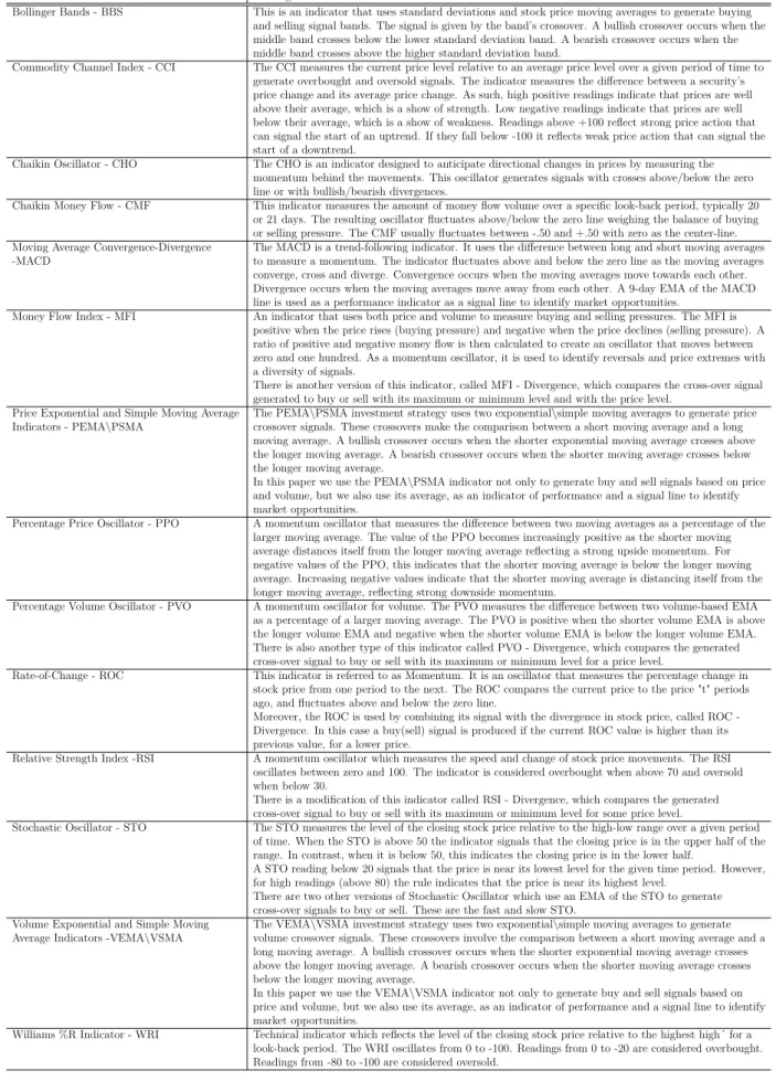
In the case of the ODS, the best 10 rules mean daily return are based on two types of TAI trading strategies. The first is a centered oscillator: the Rate-of-change indicator (ROC). The ROC is also referred to as Momentum. It is an oscillator that measures the percentage change in price from one period to the next, comparing the current price to the price "t" periods ago, and fluctuates above and below the zero line.
The second TAI is a trend-following indicator, based on the exponential moving aver-ages indicator (EMA) of the PSI 20 price Index. The EMA is a TA trading strategy that uses two exponential moving averages to generate crossover signals. These crossovers in-volve the comparison between a short moving average and a long moving average. A bullish crossover occurs when the shorter exponential moving average crosses above the longer mov-ing average. A bearish crossover occurs when the shorter movmov-ing average crosses below the longer moving average.
In the second part of Table2.4, we present the best-performance rules under the TRS.
In the TRS case, as expected, we have a higher mean daily return, 10.92 basis points (bps), and a lower number of trades than in the ODS case. In this sample, we observe that the best 10 trading rules are based on a mix of simple and complex TAI strategies. On the one hand, the best performance rule is based on the Moving Average Convergence-Divergence (MACD) indicator. The MACD is a trend-following strategy that uses the difference between long and short moving averages to identify market opportunities. The indicator fluctuates above and below the zero line as the moving averages converge, cross and diverge. Convergence occurs when the moving averages move towards each other. Divergence occurs when the moving averages move away from each other.
We also observed the presence of simple and complex EMA strategies. The complex strategy is based on the Bollinger Bands indicator (BBS). The BBS is a trading strategy
signal bands. The signal is given by the band´s crossover. A bullish crossover occurs when the middle band crosses below the lower standard deviation band. A bearish crossover occurs when the middle band crosses above the higher standard deviation band. In this set-up, the indicator combines the Index standard deviations with its exponential moving average to generate buy and sell signals.
Table 2.5 shows the profitability of our TAI trading rules for the second sub-sample
data from January 01, 2002 to August 08, 2008, where the mean buy-and-hold return is 0.0651%. In the Table, we observe for the ODS case that the t-test for the mean daily return and the difference between buy and sell mean daily returns are not significant for most of the trading rules. On the other hand, in the TRS case, only the mean daily returns are all significant.
Additionally, we also observe that the best 10 strategies in the ODS and TRS are based on a single type of TAI strategy, the ROC and the EMA, respectively. In the ODS case, the three best rules presented a significantly higher daily mean return (7.4 bps). On the other hand, in the TRS case, the best trading rules have the same performance (8.64 bps). Furthermore, we also observed a lower expected trading activity.
Table2.6shows the profitability of our TAI trading rules for the third sub-sample data
from September 01, 2008 to April 31, 2011, where the mean buy-and-hold return is -0.0596%. The results for the mean daily return and the difference between buy and sell mean daily returns are non-significant for most of the trading rules in the ODS case. Furthermore, for the TRS case the trading rules mean return and their buy-sell differences are highly non-significant.
We observe for the ODS, that the best 10 rules presented approximately the same daily mean return, from 11.17 bps to 10.07 bps, based only on the Percentage Volume Oscillator indicator (PVO). The PVO is a momentum oscillator based on volume that measures the difference between two volume-based EMA strategies as a percentage of a larger moving average.
In the second part of Table 2.6, the best 10 TAI which are also based on a variety of
TAI strategies have a mean daily return from 16.64 bps to 13.05 bps. On one the hand, we have a complex trading rule strategy based on the BBS and the Relative Strength Index (RSI). The RSI is a momentum oscillator that measures the speed and change of price movements.
On the other hand, the Percentage Price Oscillator (PPO) is a momentum oscillator that measures the difference between two moving averages as a percentage of the larger moving average. The oscillator moves into positive and negative terrain as a function of the difference between the shorter moving average and the longer moving average. Note, that contrary to previous sub-sample findings, in both types of market strategies, ODS and TRS, we verify that there is non-significant difference in the number of trades.
Table 2.7 shows the profitability of our TAI trading rules for the last sub-sample data
from May 01, 2011 to December 31, 2014, where the mean buy-and-hold return is -0.0123%. In this sub-sample, we observe that not only all mean daily returns t-test are significant,
T able 2.4: The Best 10 T AI T rading St rategies Return for the PSI-20 One-da y ahead Strategy -01/01/1993 to 31/12/2001 Mean Daily Log Return PSR Num b er of T rades PMP Strategies (P arameters) All (%) Buy (%) Sell (%) Buy-Sell (%) All (%) Buy (%) Sell (%) No. Buy No. Sell No. Neutral (%) R OC(10,0.01) 0.0897(3.45)* 0.0327(0.71) 0.1596(4.72)* -0.1268(1.51) 48.49 50,00 59,72 881 1 100 7 0.045 R OC(10,0) 0 .0895(3.44)* 0.0334(0.73) 0.1582(4.69)* -0.1248(1.49) 48.44 50.25 59.72 886 1102 0 0.045 R OC(12,0) 0 .0891(3.43)* 0.0328(0.71) 0.1583(4.69)* -0.1255(1.50) 48.79 50.87 59.94 885 1103 0 0.045 PEMA(24,26,25,0,0) 0.0883(3.40)* 0.0354(0.72) 0.1451(4.45)* -0.1097(1.23) 48.84 45.90 64.32 798 1 190 0 0.044 PEMA(24,26,50,0,0) 0.0883(3.40)* 0.0354(0.72) 0.1451(4.45)* -0.1097(1.23) 48.84 45.90 64.32 798 1 190 0 0.044 PEMA(24,26,48,0,0) 0.0883(3.40)* 0.0354(0.72) 0.1451(4.45)* -0.1097(1.23) 48.84 45.90 64.32 798 1 190 0 0.044 PEMA(24,26,35,0,0) 0.0883(3.40)* 0.0354(0.72) 0.1451(4.45)* -0.1097(1.23) 48.84 45.90 64.32 798 1 190 0 0.044 PEMA(24,26,40,0,0) 0.0883(3.40)* 0.0354(0.72) 0.1451(4.45)* -0.1097(1.23) 48.84 45.90 64.32 798 1 190 0 0.044 PEMA(24,26,45,0,0) 0.0883(3.40)* 0.0354(0.72) 0.1451(4.45)* -0.1097(1.23) 48.84 45.90 64.32 798 1 190 0 0.044 PEMA(24,26,30,0,0) 0.0883(3.40)* 0.0354(0.72) 0.1451(4.45)* -0.1097(1.23) 48.84 45.90 64.32 798 1 190 0 0.044 T rend Rev ersal Strategy Mean Daily Log Return PSR Num b er of T rades PMP Strategies (P arameters) All (%) Buy (%) Sell (%) Buy-Sell (%) All (%) Buy (%) Sell (%) No. Buy No. Sell No. Neutral (%) MA CD(5,10,16,0.1) 0.1092(4.22)* 0.0485(0.44) 0.2192(1.98)*** -0.1707( 0.82) 50.81 64.06 52.89 137 109 1742 0.619 MA CD(5,10,16,0.15) 0.1042(4.02)* 0.0428(0.41) 0.2155(2.06)*** -0.1728(0.88) 50.20 63.93 51.71 155 1 24 1709 0.588 BBS-SMA&RSI(3,0.5,0,10,75) 0.1032(3.98)* 0.0660(0.41) 0.1472(0.42) -0.0811(0.03) 48.44 40.42 68.16 1 8 1979 11.394 BBS-EMA&RSI(3,0.5,0,10,75) 0.1032(3.98)* 0.0660(0.41) 0.1472(0.37) -0.811( 0.03) 48.44 40.42 68.16 1 6 1981 14.649 BBS-SMA&RSI(3,0.5,0,10,70) 0.0981(3.78)* 0.1955(0.14) 0.1025(0.34) 0.930(0.04) 47.94 12.69 90.92 1 16 1971 5.733 BBS-EMA&RSI(3,0.5,0,10,70) 0.0981(3.78)* 0.1955(0.14) 0.1025(0.29) 0.930(0.04) 47.94 12.69 90.92 1 12 1975 7.497 BBS-EMA&RSI(3,0.5,0,15,75) 0.0964(3.66)* 0.0405(0.06) 0.1620(0.34) -0.1216(0.10) 47.33 71.27 39.32 4 6 1978 9.5 82 PEMA(5,10,0,0) 0.0949(3.61)* 0.0533(0.30) 0.1342(1.09) -0.0809(0.25) 49.35 49.75 61.97 73 73 1842 0.6 89 PEMA(5,10,35,0.015,0.015) 0.0939(3.61)* 0.0533(0.37) 0.1342(1.74) -0.0809(0.33) 48.59 37.93 70.62 114 188 1686 0.7 40 PEMA(5,10,30,0.015,0.015) 0.0939(3.13)* 0.0212(0.17) 0.1717(2.17)*** -0.1505( 0.66) 48.59 37.93 70.62 114 188 1686 0.740 Notes: The fir st column highligh ts the top 10 p erfo rmi n g T AI strategies, ba se d on the log return criteria, while the second column rep orts the mean return for these strategies. Columns 3 and 4 detail the me a n daily returns from the bu y and sell trading signals, res p ectiv ely . The B uy − S el l(%) is the difference of the mean buy and the mean sell returns. The n um b ers in paren these s are the standard t-ratios testing the returns significance and the difference of the mean buy and the mean sell returns. In columns 6 to 8, w e rep ort the P S R whic h is the n um b er of times that our T AI trading rule esti ma tio n matc hes the real mark et mo v emen t for eac h sub-sample in v estme n t time horizon. The Al l(% , B uy (% and S el l(% are resp ectiv e ly the o v erall p ercen tage, buy and se ll correct signals rep orted in the sample. A dditionally , N o.B uy and N o.S e ll are the total n um b e r of buy and se ll trades resp e ctiv ely . Finally , in the last column w e presen t the “p oten tial margins fo r profita bi lit y” (P M P %) as suggested b y Hsu et al. (2010). That is, the break-ev en transaction cost v alues that eliminate an y out-p erformance. *** Statistical Significance at the 10% lev el for a tw o-tailed test. **Statistical Significance at the 5% lev el.*Statistical Significance at the 1% lev el.
T able 2.5: The Best 10 T AI T rading St rategies Return for the PSI-20 One-da y ahead Strategy -01/01/2002 to 3 0/08/2008 Mean Daily Log Return PSR Num b er of T rades PMP Strategies (P arameters) All (%) Buy (%) Sell (%) Buy-Sell (%) All (%) Buy (%) Sell (%) No. Buy No. Sell No. Neutral (%) R OC(10,0) 0.0740(3.63)* 0.01674(0.39) 0.1230(4.84)* -0.1063( 1.56) 46.72 36.52 69.67 324 667 0 0.037 R OC(10,0.01) 0.0737(3.62)* 0.0159(0.37) 0.1231(4.84)* -0.1072(1.56) 46.72 36.24 69.67 322 667 2 0.037 R OC(10,0.2) 0.0 733(3.68)* 0.0205(0.45) 0.1281(4.86)* -0.1076( 1.50) 45.31 33.70 66.11 300 625 66 0.039 R OC(5,0.2) 0.0396(2.02)*** -0.0250(0.54) 0.0961(3.45)* -0.1207( 1.64) 42.68 33.10 57.95 300 572 11 9 0.022 R OC(5,0) 0.0388(1.90) -0.0410(1.02) 0.0977(3.73)* -0.1390(2.09)*** 44.6 0 38.20 64.02 356 635 0 0.019 R OC(5,0.025) 0.0377(1.85) -0.0430(1.05) 0.0988(3.71)* -0.1418(2.10)*** 44.40 37.64 62.76 349 619 23 0.019 R OC(5,0.01) 0.0 375(1.83) -0.0420(1.04) 0.0968(3.67)* -0.1391(2.08)*** 44.40 37.92 63.39 353 628 10 0.019 R OC(5,0.15) 0.0 373(1.87) -0.0250(0.56) 0.0900(3.25)* -0.1151(1.60) 43.09 35.39 58.79 314 588 89 0.021 R OC(5,0.1) 0.0370(1.84) -0.0280(0.6 5) 0.0896(3.2 9)* -0.1176(1.66) 43.59 36.00 60.25 323 600 68 0.020 R OC(5,0.05) 0.0 358(1.76) -0.0410(1.00) 0.0948(3.52)* -0.1362(1.99)*** 43.79 37.08 61.51 343 611 37 0.019 T rend Rev ersal Strategy Mean Daily Log Return PSR Num b er of T rades PMP Strategies (P arameters) All (%) Buy (%) Sell (%) Buy-Sell (%) All (%) Buy (%) Sell (%) No. Buy No. Sell No. Neutral (%) PSMA(5,12,25,0.01,0.01) 0.0864(4.25)* 0.0356(0.38) 0.1410(1.9 5) -0.1053(0.64) 48.23 42.42 68.41 68 80 843 0.599 PSMA(5,10,25,0.01,0.01) 0.0864(4.25)* 0.0356(0.38) 0.1410(1.9 5) -0.1053(0.64) 48.23 42.42 68.41 68 80 843 0.599 PSMA(5,10,120,0.01,0.01) 0.0864(4.25)* 0.0356(0.38 ) 0.1410(1.95) -0.1053(0.64) 48.23 42.42 68.41 68 80 84 3 0.599 PSMA(5,12,30,0.01,0.01) 0.0864(4.25)* 0.0356(0.38) 0.1410(1.9 5) -0.1053(0.64) 48.23 42.42 68.41 68 80 843 0.599 PSMA(5,10,80,0.01,0.01) 0.0864(4.25)* 0.0356(0.38) 0.1410(1.9 5) -0.1053(0.64) 48.23 42.42 68.41 68 80 843 0.599 PSMA(5,10,20,0.01,0.01) 0.0864(4.25)* 0.0356(0.38) 0.1410(1.9 5) -0.1053(0.64) 48.23 42.42 68.41 68 80 843 0.599 PSMA(5,10,70,0.01,0.01) 0.0864(4.25)* 0.0356(0.38) 0.1410(1.9 5) -0.1053(0.64) 48.23 42.42 68.41 68 80 843 0.599 PSMA(5,10,55,0.01,0.01) 0.0864(4.25)* 0.0356(0.38) 0.1410(1.9 5) -0.1053(0.64) 48.23 42.42 68.41 68 80 843 0.599 PSMA(5,10,60,0.01,0.01) 0.0864(4.25)* 0.0356(0.38) 0.1410(1.9 5) -0.1053(0.64) 48.23 42.42 68.41 68 80 843 0.599 PSMA(5,10,90,0.01,0.01) 0.0864(4.25)* 0.0356(0.38) 0.1410(1.9 5) -0.1053(0.64) 48.23 42.42 68.41 68 80 843 0.599 Notes: The first column highligh ts the top 10 p erforming T AI strategies, based on the log return criteria, while the second column rep orts the mean return for these strategies. Columns 3 and 4 detail the mean daily return from the buy and sell trading signals, resp ectiv el y . The B uy − S el l(%) is the difference of the mean buy and the mean sell returns. The n um b ers in paren these s are the standard t-ratios testing the returns significance and the difference o f the mean buy and the mean sell returns. In columns 6 to 8, w e rep ort the P S R whic h is the n um b er of times that our T AI trading rule estim a ti o n matc hes the real mark et mo v emen t for eac h sub-sample in v estmen t time horizon. The Al l(% , B uy (% and S el l(% are resp ectiv ely the o v erall p ercen tage, buy a nd sell correct signals rep orted in the sampl e. A dditionally , N o.B uy and N o.S el l are the total n um b er of buy and sell trades resp ectiv ely . Finally , in the last column w e p re sen t the “p oten tial margins for profitabilit y” (P M P %) as suggested b y Hsu et al. (2010 ). That is, the break-ev en transaction cost v alues that eliminate an y out-p erformance. *** Statistical Significance at the 10 % lev el fo r a tw o-tailed test. **Statistical Significance at the 5% lev el.*Statistical Significance at the 1% lev el.