A Work Project, presented as part of the requirements for the Award of a Masters Degree in Finance from the NOVA – School of Business and Economics.
Differences in the prices of physical ETF’s and synthetic ETF’s
Diogo André Pereira Alves Nunes, #392
A Project carried out on the Finance course, under the supervision of: Professor Miguel Ferreira
2
Abstract
Exchange Traded Funds, ETF’s, are a relatively recent investment product that observed high growing in the last decade. They bring investors some advantages, but might also
have some disadvantages, depending on the investor profile. In this piece of research,
the pricing mechanism of ETF’s is exhaustively dissected and it is compared with external factors that influence ETF’s prices, namely volatility, in order to determine if there is a relationship between them and if volatility is a good explanatory variable for
ETF’s prices.Also, the pricing mechanism of two different types of ETF’s is compared, physical ETF’s and synthetic ETF’s, in order to determine if there are any significant differences between both of them.
3
Index
Abstract ... 2
1. Introduction ... 4
2. Exchange Traded Funds (ETF’s) Definition ... 6
3. Physical Replication Vs. Synthetic Replication ... 10
4. Pricing Mechanism and Arbitrage Opportunities... 14
5. Data Analysis ... 19
6. Conclusions ... 25
4
1.
Introduction
Exchange Traded Funds, ETF’s, are a type of funds, just like mutual funds, but with some special characteristics, the most important of them is that they trade like a stock
and they are conceived to track an underlying performance, rather than beating a
benchmark, has it is the case of mutual funds.
There are two main types of ETF’s, physical ETF’s and synthetic ETF’s. The difference between them lies in the way they replicate the underlying performance: by owning the
underlying, in the case of physical replication, or through derivatives and swaps, in the
case of synthetic replication.
ETF’s are traded in stock exchanges, so their price is influenced by supply and demand factors, just like any other stock (with some important differences that will be addressed
later on).
The pricing mechanism of ETF’s suggests that volatility might be an important factor to take into account, when studying ETF’s prices. It also suggests that there might be a difference between the pricing of physical ETF’s and synthetic ETF’s, and that volatility might influence both of them in different ways.
In this research, the main objective was trying to find evidence for the ideas suggested
above, by analyzing real data from a large sample of ETF’s and relate it with market volatility to find out if effectively there is a relationship between both, and how
5
After all the analysis was made, it was observed that there is an effective relation
between market volatility and ETF’s prices, and this relation is different for physical and synthetic ETF’s.
This difference is caused by the pricing mechanism mentioned, and the reason for that is
that the higher the volatility, the less efficient this mechanism is and ETF prices are less
6
2.
Exchange Traded Funds (ETF’s)
Definition
ETF’s are a relatively recent investment vehicle, but in less than 20 years they have become one of the most popular choices between investors. The first attempt of
launching something similar to an ETF occurred in 1989, but only in 1993 the first ETF
was successfully created and started trading in January of that year.
With the uprising of financial markets and the spread of information, investors became
more and more informed and sophisticated, and started looking to alternative
investments and asset classes. However, investing in these alternative vehicles, rather
than the conventional ones, proved to be sometimes very difficult, or even impossible.
ETF’s offer an easy and accessible exposure to almost every asset class and region in the world, weather it is equities, commodities, foreign exchange, interest rate or debt.
As the name suggests, an Exchange Traded Fund is a fund that, unlike a mutual fund, is
traded in stock exchanges just like a regular stock. This way, investors can very easily
buy or sell their participation in the fund, and realize gains or change their investing
perspective and market vision, from one asset class to another.
As mutual funds have already been mentioned above, it makes sense, in order to better
understand what is an ETF, to make a comparison between ETF’s and mutual funds, and talk about the advantages and disadvantages of the first ones when compared to the
second ones, and when compared to investing directly in the underlying of the funds.
On the advantages side, the following are the most relevant ones:
- Diversification: ETF’s offer an easy way to diversify the investments; for
7
by an ETF that tracks this index, instead of buying all its constituent shares in
the appropriate proportions. The same happens when an investor wants to be
exposed to a specific region of the world, a specific sector, etc.
- Low management fees: Unlike mutual funds, ETF’s are passively managed,
since their objective is not to beat a benchmark but instead to track it, whereas in
mutual funds, the goal is to beat the benchmark. This implies that mutual funds
need to be actively managed, in order to reach their objectives, which requires
higher management fees to be paid by investors.
- Trade like a stock:As mentioned before, ETF’s are traded in stock exchanges.
This provides investors all the advantages of trading stocks, like selling short, or
manage risk by trading futures and options over ETF’s. Also, an investor can be updated throughout the day about the valuation of it fund, unlike the case of a
mutual fund, in which the price is only published at the end of the day at its Net
Asset Value (NAV; we will deepen this concept in part 4). This gives investors
more information about the worthiness of intraday trading, in a more volatile
market session.
Depending on the profile of the investor, ETF’s might have some disadvantages, when compared to investing in mutual funds or directly in the underlying; the following are
the most relevant ones:
- Intraday pricing might be a disadvantage: If an investor has a long time
horizon, high hourly swings in the price of ETF’s might trigger trades, that otherwise would not happen in the case of mutual funds, since their price is only
published at the end of day; this way, high hourly swings could cancel out
8
investment objective. In the long run, high intraday changes in the price of
ETF’s will not have a significant impact on the investment return, which is what long term investors are looking for.
- Might be more expensive: As mentioned above, one of ETF’s advantages are their lower management fees when compared to mutual funds, since they are
passively managed funds. However, when compared to investing directly in the
underlying of the ETF’s (for example, buying stocks, or buying commodities), ETF’s are more expensive because although their management fees are lower than mutual funds, there is still a price to pay, whereas when buying directly the
underlying, only transaction fees are paid, which are also included in the ETF’s management fees.
- Riskier: Depending on the risk profile of the investor this characteristic of some
ETF’s might be a disadvantage. There are some specific types of ETF’s that leverage the returns of the underlying (double or triple leveraged ETF’s, for example). This means that the gains in the ETF’s will be higher than the appreciation of the underlying, but also the losses are higher than the
depreciation of the underlying. For investor with a risk lover profile, usually
more informed investors, this can be seen has an advantage, but for a more
conservative investor, this might represent a big disadvantage and risk.
- Lower dividend yields:There are dividend paying ETF’s, which aggregate the
dividends paid by the constituent stocks of the index tracked by the ETF. As this
aggregated dividend is calculated through a weighted average of the relative
weights of every component of the index, the dividend will be lower than the
9
looking for a dividend paying alternative and can take on the risk of owning
only the high-yielding stocks, abdicating the diversification effect provided by
the index tracking fund, than it might be better to buy the stocks than owning the
10
3.
Physical Replication Vs. Synthetic Replication
As mentioned before, ETF’s objective is to track the performance of its underlying asset, weather it is a stock index, a commodity, a foreign exchange parity, etc. In order
to do this, ETF managers have two options: they can use a physical replication
approach, Physical ETF’s, or choose to do it by synthetically replicate the returns, Synthetic ETF’s.
In the case of physical replication, the ETF management company actually buys the
underlying and holds it, in order to benefit from its returns. For example, if an ETF
tracks a stock index, say the S&P500, the management company buys each one of the
stocks composing the index, in the same relative proportions. If we have an ETF that
tracks a commodity, say gold, the management company buys and stores gold and
benefits from its appreciation, replicating those returns in the ETF.
On the other hand, when we have a synthetic replicating strategy, there are no physical
underlying involved; their performance is replicated by using derivative or futures
contracts, or by entering into swap agreements with counterparties that guarantee the
performance of the underlying, in exchange for a swap spread paid by the management
company.
There are ETF managers who prefer to follow the Physical Replication method and
there are others who prefer to do it using Synthetic Replication, but both of them have
some advantages and disadvantages. Some ETF’s track underlyings that are very illiquid; this makes Physical Replication very hard to achieve, so Synthetic Replication
is a solution in these cases. On the other hand, since on the second case we are
11
performance, Synthetic Replicating ETF’s are exposed to counterparty risk, which is almost inexistent in the case of Physical Replicating ETF’s.
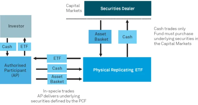
To illustrate the mechanism of these two replication ways, the following figure shows
the structure of a physically replicating ETF:
Figure 1: A Physically Replicating ETF (Source: Blackrock)
An Authorized Participant (AP), is an entity, generally large broker-dealers, that act as
market makers of the ETF, taking or delivering units of the fund into the market.
As we can see in figure 1, the ETF managers receive cash from investors (through the
AP’s), which then use to buy the underlying of the fund, in order to be exposed to its performance and reflect that performance in the ETF. Also, the AP’s can, instead of paying the fund managers directly the cash from investors, buy the underlying on the
market and then give it to the ETF managers in exchange for the ETF shares. This
process will be addressed later on, when we approach the pricing mechanism and
12
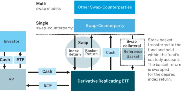
For the synthetic replicating ETF’s, we have two models, the Unfunded Swap Model and the Fully Funded Swap Model. In the first case the ETF manager “buys” from a counterparty a reference basket of securities, that generally is not related with the
replicating index, and then swaps with the counterparty the performance of the
reference basket by the performance of the underlying (figure 2). In this case, the
counterparty risk is associated with the difference between the NAV of the fund and the
value of the reference basket, because in case of a counterparty default, the ETF
managers will use the reference basket to pay investors.
Figure 2: A Synthetic Replicating ETF – Unfunded Swap Model (Source: Blackrock)
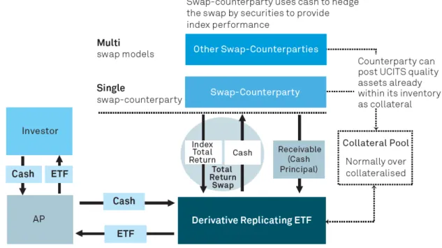
In the case of the Fully Funded Swap Model, the ETF managers transfer the notional
amount of the fund to the counterparty, which in return guarantees the underlying
performance and place with a third party a collateral pool, which is accessed by the ETF
managers in case of a counterparty default (figure 3). This collateral pool is generally
13
between the Unfunded Swap Model and the Fully Funded Swap Model is the
overcollateralization, in the second case.
14
4.
Pricing Mechanism and Arbitrage Opportunities
One of the most commonly known phrases that describe ETF’s is “They trade like a stock”; this means that after being issued, their price is ruled only by supply and demand effects. So, a question arises: What makes their price always trade so close to
their Net Asset Value, NAV? Before answering that question, we should define what
the NAV of an ETF is. As in any other fund (also mutual funds), the NAV of an ETF is
determined by dividing the value of its holdings by the number of shares outstanding.
When issued, an ETF is sold at its NAV, but after that its only supply and demand
effects that rule its price. When the price of an ETF is trading above its NAV, we say
the ETF is trading at a premium; if the opposite happens, than the ETF is trading at a
discount. If suddenly the demand for a specific ETF increases drastically, that would
cause its price to jump. However, if its holdings remain unchanged, also does its NAV,
and that means that the ETF would be trading at a large premium. When the price of
ETF’s deviate from its NAV, at a certain point an arbitrage opportunity is created; AP’s then, benefit from this arbitrage causing the ETF price to converge again to its NAV.
To explain how this arbitrage mechanism works, first we need to say that, at the
beginning of each day, the ETF managers provide a description of a basket of securities
they are willing to take from AP’s in exchange for issuing a new share of the ETF, or the opposite, redeeming an ETF share in exchange for the same basket of securities.
This is valid for the case of Physical ETF’s; in the case of Synthetic ETF’s, instead of the basket of securities the ETF managers determine an amount in cash they are willing
to take in exchange for an ETF share, which is then used to buy the derivatives or swaps
15
In the case of a physical ETF, the NAV of the fund will be closely related to the price of
its underlying; the NAV will always be equal to the mid price of the basket of securities
equivalent to one share of the fund. Consequently, the price of the ETF tends to trade
between the bid/ask spread of the basket of underlyings. If the ETF price diverges
sufficiently from the NAV, above the underlying ask price or bellow its bid price, than
an arbitrage opportunity is created: for example, if the ETF price is trading above the
ask price of the underlying, an AP can sell an ETF share and buy the corresponding
basket of securities. At the end of the day, the ETF managers will accept the basket of
securities and issue a new ETF share in exchange, which is then used to settle the sale
of the share made during the day. The profit is the difference between the ETF price and
the underlying ask price, at the time of the trade (if we exclude trading costs). When the
ETF price drops below the bid price of the underlying, the same arbitrage occurs, but
working the opposite way; an AP can now buy a share of the ETF from the market and
sell the equivalent basket of securities. At the end of the day, the ETF managers will
accept to redeem the ETF share in exchange for its corresponding basket of securities,
which is then used to settle the sale of the basket.
For synthetic ETF’s, the process works similarly but with a slight difference, besides the fact that instead of having a basket of securities we have an amount in cash, has
mentioned before; due to the fact that the settlement is only made at the end of the day,
the cash amount equivalent to selling or buying an ETF share during the day might be
different from the amount needed to buy or sell derivatives equivalent to that share at
the end of the day, because the counterparty will only quote the derivatives, or swap at
the end of day, which is when the ETF managers exchange cash and ETF shares with
16
benefit from the arbitrage, until the end of the day, so does the price of the derivatives.
This means that the AP’s are exposed to a risk between the arbitrage trading and the end of the day. They can, and do, edge that risk, but that edging has a cost. This means that
for an arbitrage to happen in the case of synthetic ETF’s, the difference between the ETF price and the underlying price must be a bit higher than in the case of physical
ETF’s, in order to cover for the hedging costs.
This study focuses on the differences between the premiums/discounts of physical
ETF’s and Synthetic ETF’s, and then tries to relate the differences observed with market volatility, in order to understand if this factor influences the differences in the
prices of physical and synthetic ETF’s. Thus, in order to understand the conclusions presented later, we should first understand the volatility effects in the pricing of ETF’s.
Volatility affects ETF’s pricing in two main ways; the first one applies to both physical and synthetic ETF’s, and the second one applies to the synthetic ETF’s pricing mechanism.
First, as we mentioned before, for an arbitrage opportunity to arise, the ETF price must
trade outside the bid/ask spread of the underlying. When we have low market volatility,
the underlying bid/ask price will be easier and more accurately determined. In figure 4,
we can see an ETF price trading between the underlying bid/ask lines, perfectly
17
Figure 4: Underlying Bid/Ask under low market volatility conditions (Source: Blackrock)
When market volatility increases, there is more uncertainty surrounding the underlying
price, and the perfectly determined bid/ask lines of figure 4 will turn into “bands” of possible prices for the underlying (figure 5).
Figure 5: Underlying Bid/Ask under high market volatility conditions (Source: Blackrock)
In this case, it is harder to accurately price the underlying, and the difference between
the prices of the ETF and the underlying will need to be a bit higher, in order to cover
for the uncertainty surrounding the underlying price, and guarantee that the arbitrage
18
we expect that when volatility increases, so does the ETF’s premium/discount, because this difference needs to be higher for arbitrage to be profitable.
The second volatility effect is more related with the pricing mechanism of synthetic
ETF’s. As we mentioned before, in the case of synthetic ETF’s there are hedging costs that need to be considered, in order to cover for the risk of the underlying price variation
during the day, from the moment when the arbitrage is traded until it is settled, at the
end of day, which will also affect the price of the derivatives and swaps on the
underlying, and finally change the amount of cash needed to create or redeem an ETF
share. In periods of high market volatility, this daily changes in the price of the
underlying will also be higher, and so it will be the hedging costs. As the hedging costs
increase, so it does the difference between the ETF price and the underlying bid/ask, in
order for the arbitrage to be profitable. Thus, due to this effect we expect that the ETF
premium/discount increases with market volatility.
In conclusion, and taking into account what was mentioned above, we would expect to
see a higher ETF premium/discount in periods of high market volatility, especially in
19
5.
Data Analysis
In order to study the differences in the prices of physical ETF’s and synthetic ETF’s, a large sample of ETF’s was used; the data used consisted of daily prices and NAV’s for a set of over 2600 physical ETF’s and 4500 synthetic ETF’s. For a period of 7 years, from the beginning of 2005 until the end of 2011, the daily premium/discount was
calculated for each ETF, using the following expression:
For each day, an average of the deviations from NAV was calculated in order to obtain
the daily average premium/discount, separately for synthetic ETF’s and physical ETF’s.
With this procedure, two series of data were obtained: the daily average
premium/discount for synthetic ETF’s, with a 7 years length, and the same series for physical ETF’s. The goal now was to analyze these series, relate them with market volatility and try to identify if what was expected to be observed, based on the
theoretical background previously exposed, was in fact observed in the real world. But
before that, the data needed to be cleaned from every extreme value (outliers) that could
bias the analysis. To do that, the 10% extreme values of the deviations from NAV on
each day, positive and negative (premiums and discounts) were eliminated, and only the
middle values, 80% of the total, were used. The decision of eliminating 10% of the
values on each extreme was taken, because with the exclusion of less than 10% on each
tail the data was still very “noisy”.
The goal now was to compare the values obtained with market volatility. To measure
20 -1,50%
-1,00% -0,50% 0,00% 0,50% 1,00% 1,50% 2,00%
14-01-2004 28-05-2005 10-10-2006 22-02-2008 06-07-2009 18-11-2010 01-04-2012 14-08-2013
P/D (%)
Premium/discounts and VIX - S&P500 volatility index
Physical
Synthetic
VIX
reflects an estimation of the future volatility of the S&P500 index, and it is a good
estimation for overall market volatility. A series with the same frequency and length of
the daily deviations from NAV was used (daily values from 2005-2011).
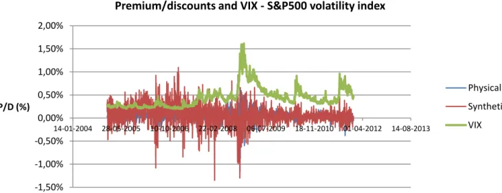
In figure 6, we can see the three series of data obtained:
Figure 6: ETF’s premiums and discounts
Simply from observing the previous figure there is not much to conclude, so, two linear
regressions were made, to see if VIX might be an explanatory variable of the
premiums/discounts for both types of ETF’s.
Tables 1 and 2 show the results obtained for both regressions:
Tables 1 and 2: Results of two linear regression, with the VIX as independent variable and
21
As we can see from the data above, in the case of physical ETF’s, VIX is not an explanatory variable for the premiums/discounts, due to its p-value of 0,4297 (higher
than 0,05, which means that for a 5% significance level we do not reject the null
hypothesis that the VIX coefficient in the regression is equal to zero). In the case of the
synthetic ETF’s, although the VIX coefficient has a p-value equal to zero, which would indicate this as an explanatory variable, the adjustment of the regression is very poor (as
it is in the case of the physical ETF’s), with an R2 of 0,052565, which means that only 5,2565% of the premiums/discounts are explained by the VIX.
So far, we can see that there is no apparent relation between the volatility and the value
of the deviations from NAV, positive or negative. But from the theoretical background
previously exposed, it seems reasonable to expect that volatility might influence the
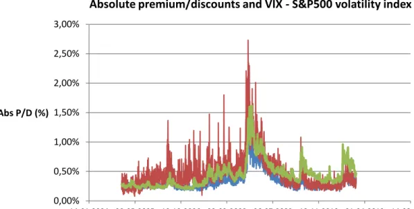
premiums/discounts of ETF’s, so the same above analysis was done, but considering absolute values for the premiums/discounts. This way, we are only considering
deviations from NAV, not taking into account if they are positive or negative
(premiums or discounts), and we will try to observe if there is a relation between the
volatility and the absolute deviations of ETF’s prices from their NAV. This seems to be a reasonable consideration, because, as it was explained before, the arbitrage
mechanism works similarly either if we have a premium or a discount only the opposite
way, and the volatility impact is the same in each case.
Figure 7 shows the same results as before, but with the absolute values of
22 0,00%
0,50% 1,00% 1,50% 2,00% 2,50% 3,00%
14-01-2004 28-05-2005 10-10-2006 22-02-2008 06-07-2009 18-11-2010 01-04-2012 14-08-2013
Abs P/D (%)
Absolute premium/discounts and VIX - S&P500 volatility index
Physical
Synthetic
VIX
Figure 7: ETF’s absolute premiums and discounts
From the observation of the previous graphic, it seems that there is a much closer
relation between the absolute deviations and the VIX, and that these deviations are
higher for the synthetic ETF’s than for the physical ETF’s. To test if these observations are actually making sense, same both regressions as before were made. The results are
presented in tables 3 and 4 below:
Tables 3 and 4: Results of two linear regression, with the VIX as independent variable and absolute
premiums/discounts as dependent variable
Now we can see that the p-values for the VIX variable are equal to zero in both
regressions, so we exclude the null hypothesis that the VIX coefficient is equal to zero,
23 y = 0,0001x + 0,0004
R² = 0,7273
0,00% 0,40% 0,80% 1,20% 1,60% 2,00%
- 20,00 40,00 60,00 80,00 100,00
A b s P/D (% ) VIX Physical
y = 0,0002x + 0,0008 R² = 0,472
0,00% 0,50% 1,00% 1,50% 2,00% 2,50% 3,00%
- 20,00 40,00 60,00 80,00 100,00
A b s P/D (% ) VIX Synthetic
means that the VIX might be an explanatory variable for the absolute deviations of ETF
prices from their NAV’s. These regressions are illustrated in figures 8 and 9:
Figures 8 and 9: Graphic illustration of the linear regression, with the VIX as independent variable
and absolute premiums/discounts as dependent variable
We can also observe that the VIX coefficient is higher for the synthetic ETF’s regression than in the case of the physical ETF’s. This is in line with what was previously expected, when it was mentioned that the volatility has a double effect in the
arbitrage mechanism, in the case of the synthetic ETF’s, and that was expected to cause a higher deviation between synthetic ETF’s price and their NAV, than for the physical ones.
So far, the conclusions from the analysis made seem to make sense and be in line the
theoretical background. However, the results obtained so far could be biased by some
effect happening in a specific type of ETF’s; the data series used, with the absolute deviations for physical and synthetic ETF’s were composed of daily average values of the deviations for every type of ETF’s, only distinguishing between physical and synthetic. Let’s imagine that the behavior observed so far was in reality only observed in a more specific type of ETF, but in a large scale, causing this effect to propagate to
24
underlyings, globally. So, in order to determine if the behavior observed is transversal
to all asset classes and regions, the daily absolute premiums/discounts were divided into
three types of underlying asset classes, equity, fixed income and commodities, the most
significant ones, and also by domicile regions, Americas, Europe, Asia-Pacific and
Africa, but always making the distinction between physical and synthetic ETF’s.
The results showed that the effect observed in the main analysis is generalized through
all regions and asset classes: the absolute premiums/discounts are higher when volatility
increases, and this effect is accentuated in the case of synthetic ETF’s, as we can see on table 5, from the average and median values for both type of ETF’s premiums/discounts, on each year.
Table 5: Average and median premiums/discounts and VIX
Year Average Median
Physical Synthetic VIX Physical Synthetic
2005 0,2503% 0,3025% 12,78 0,2482% 0,2878%
2006 0,2689% 0,4255% 12,80 0,2512% 0,3913%
2007 0,2781% 0,4917% 17,50 0,2607% 0,4398%
2008 0,5375% 0,8253% 32,58 0,4077% 0,6621%
2009 0,4639% 0,6322% 31,48 0,4308% 0,5759%
2010 0,2669% 0,3106% 22,55 0,2527% 0,2852%
25
6.
Conclusions
The main objectives of this study were to observe the behavior of the prices of physical
and synthetic ETF’s, the differences between them and how are they influenced by volatility.
After fully understanding how ETF’s are priced and the details of their pricing mechanism, some results were expected beforehand analyzing the data.
First, it was expected that volatility would have a significant impact on ETF’s premiums and discounts. In fact, by analyzing the results previously presented, it is possible to see
that volatility actually has an impact on the divergence of ETF’s prices from their NAV: ETF’s absolute premiums or discounts increase with volatility. Most importantly, it was interesting to see how differently, volatility would influence the prices of physical
ETF’s and synthetic ETF’s, separately. The results indicate that synthetic ETF’s are more sensitive to variations in volatility, and its increase causes higher price deviations
from NAV in the case of synthetic ETF’s, than in physical ETF’s.
Although so far this analysis produced some decent conclusions, there was one thing for
which inconclusive results were obtained: we saw that volatility influences the absolute
deviations of ETF prices from their NAV, but are these deviations premiums or
discounts?! In fact, with the analysis produced, there was no evidence that volatility
would have an impact on premiums or discounts, but rather in their absolute value. In
other words, we know that in more volatile periods ETF’s tend to trade at larger deviations from their NAV, especially synthetic ETF’s, but we don’t know if the deviations tend to be positive or negative, it was rather observed that there can be
26
These conclusions are in line with the expectations: from the moment ETF’s are launched in the market, their price fluctuates just like a stock, influenced by supply and
demand, but with the difference that in the case of ETF’s there is an arbitrage mechanism that restrains the behavior of ETF prices, namely it controls the difference
between ETF prices and their NAV.
In periods of higher market volatility, ETF’s prices tend to trade at higher premiums/discounts, which means that these arbitrage mechanisms are less efficient in
27
7.
Bibliography
Aggarwal, Reena. 2012. The Growth of Global ETFs and Regulatory Challenges.
Georgetown University, McDonough School of Business: Center for Financial Markets
and Policy.
Poterba, James M.; Shoven, John B. 2002. Exchange Traded Funds: A new
investment option for taxable investors. Massachusetts Institute of Technology:
Department of Economics.
Petajisto, Antti. 2011. Inefficiencies in the Pricing of Exchange-Traded Funds. NYU,
Stern School of Business.
Meinhardt, Christian; Müller, Sigrid; Schöne, Stefan. 2012. Synthetic ETFs: Is
physical replication dead? Humboldt-University of Berlin, School of Business and
Economics: Institute of Finance.
Ramaswamy, Srichander. 2011. “Market structures and systemic risks of exchange-traded funds.”Bank for International Settlements Working Papers, No 343.
2011. Potential financial stability issues arising from recent trends in Exchange-Traded
Funds (ETFs). Financial Stability Board.
Newlands, Chris. 2011. “Physical vs synthetic debate is hotting up.” Financial Times.
ETP Due Diligence - A Framework to Help Investors Select the Right European