Proceedings of Modern Heuristic for Decision Support, pp. 67–81,UNICOM seminar, 18–19 March 1997,London
Genetic Algorithms for Job-Shop
Scheduling Problems
Takeshi Yamada and Ryohei Nakano
NTT Communication Science Labs.
2 Hikaridai, Seika-cho, Soraku-gun, Kyoto 619-02 JAPAN
E-mail:
{
yamada,nakano
}
@cslab.kecl.ntt.co.jp
1
Introduction
Then×mminimum-makespangeneral job-shop scheduling problem, hereafter referred to as the JSSP, can be described by a set ofn jobs{Ji}1≤j≤n which is to be processed on a
set of m machines {Mr}1≤r≤m. Each job has a technological sequence of machines to be
processed. The processing of jobJj on machineMr is called theoperationOjr. Operation
Ojrrequires the exclusive use ofMr for an uninterrupted durationpjr, its processing time.
A schedule is a set of completion times for each operation {cjr}1≤j≤n,1≤r≤m that satisfies
those constraints. The time required to complete all the jobs is called the makespan
L. The objective when solving or optimizing this general problem is to determine the schedule which minimizes L. An example of a 3×3 JSSP is given in Table 1. The data includes the routing of each job through each machine and the processing time for each operation (in parentheses). Figure 1 shows a solution for the problem represented by “Gantt-Chart”.
Table 1: A 3×3 problem
job Operations routing (processing time)
1 1 (3) 2 (3) 3 (3)
2 1 (2) 3 (3) 2 (4)
3 2 (3) 1 (2) 3 (1)
The JSSP is not only N P-hard , but it is one of the worst members in the class. An indication of this is given by the fact that one 10×10 problem formulated by Muth and Thompson [15] remained unsolved for over 20 years.
1.1
Disjunctive graph
The JSSP can be described by a disjunctive graphG= (V, C∪D), where (1) V is a set of nodes representing operations of the jobs together with two special nodes, a source(0) and a sink ⋆, representing the beginning and end of the schedule, respectively. (2) C is a set of conjunctive arcs representing technological sequences of the operations. (3)D is
M1
?? ?? ??J
2 ????
J
1? ? ? ?
J
3M
2 ??????????
J
2??
??
J
1M3
??? ???J
2 ? ? ? ? ?J
3 ??? ???J
1 time0 2 4 6 8 10 12
?? ?? ??
J
3Figure 1: A Gantt-Chart representation of a solution for a 3×3 problem
a set of disjunctive arcs representing pairs of operations that must be performed on the same machines. The processing time for each operation is the weighted value attached to the corresponding nodes. Figure 2 shows this in a graph representation for the problem given in Table 1.
O11 O12 O13
O21 O23 O22
O31
O32
p = 312
33
O
13
p = 3
31
p = 2
32
p = 3 p = 133
21
p = 4
22
p = 2
11
p = 3
23
p = 3
*
sink source
conjunctive arc (technological sequences)
disjunctive arc (pair of operations on the same machine)
O
ij : an operation of job i on machine j
: processing time of O
pij ij
0
Figure 2: A disjunctive graph of a 3×3 problem
Job-shop scheduling can also be viewed as defining the ordering between all operations that must be processed on the same machine, i.e. to fix precedences between these opera-tions. In the disjunctive graph model, this is done by turning all undirected (disjunctive) arcs into directed ones. Aselectionis a set of directed arcs selected from disjunctive arcs. By definition, a selection iscompleteif all the disjunctions are selected. It is consistent if the resulting directed graph is acyclic.
1.2
Semi-active schedules
algorithm 1 GT algorithm
1. Let D be a set of all the earliest operations in a technological sequence not yet scheduled andOjrbe an operation with the minimumECinD: Ojr = arg min{O ∈
D|EC(O)}.
2. Assume i−1 operations have been scheduled onMr. Aconflict setC[Mr, i] is defined
as: C[Mr, i] ={Okr∈D|Okr on Mr, ES(Okr)< EC(Ojr)}.
3. Select an operation O ∈C[Mr, i] arbitrary.
4. Schedule O as the i-th operation onMr with its completion time equal to EC(O).
and is composed of a sequence of critical operations. A sequence of consecutive critical operations on the same machine is called a critical block.
The distance between two schedules S and T can be measured by the number of differences in the processing order of operations on each machine [16]. In other words, it can be calculated by summing the disjunctive arcs whose directions are different between
S and T. We call this distance the disjunctive graph (DG) distance. Figure 3 shows the DG distance between two schedules. The two disjunctive arcs drawn by thick lines in schedule (b) have directions that differ from those of schedule (a), and therefore the DG distance between (a) and (b) is 2.
DG distance = 2
O11 O12 O13
O21 O23 O22
O31
O32 O33
* 0
(a) O11 O12 O13
O21 O23 O22
O31
O32 O33
* 0
(b)
Figure 3: The DG distance between two schedules
1.3
Active schedules
The makespan of a semi-active schedule may often be reduced by shifting an operation to the left without delaying other jobs. Such reassigning is called a permissible left shift
and a schedule with no more permissible left shifts is called an active schedule. An optimal schedule is always active so the search space can be safely limited to the set of all active schedules. An active schedule is generated by the GT algorithm proposed by Giffler and Thompson [12], which is described in Algorithm 1. In the algorithm, the earliest starting time ES(O) and earliest completion time EC(O) of an operation O
2
Simple GAs with binary representation
As described in the previous section, a (semi-active) schedule is obtained by turning all undirected disjunctive arcs into directed ones. Therefore, by labeling each directed disjunctive arc of a schedule as 0 or 1 according to its direction, a schedule can be represented by a binary string of lengthmn(n−1)/2. Figure 4 shows a labeling example, where an arc connecting Oij and Okj (i < k) is labeled as 1 if the arc is directed from Oij
toOkj (so Oij is processed prior to Okj) or 0, otherwise. It should be noted that the DG
distance between schedules and the Hamming distance between the corresponding binary strings can be identified through this binary mapping.
O11 O12 O13
O21 O23 O22
O31
O32 O33
*
0
0
0
0
0
0
0
1
1
1
1
1
1
1
1
1
1
1
1
Figure 4: Labeling disjunctive arcs
A conventional GA using this binary representation was proposed by Nakano and Yamada [16]. An advantage of this approach is that conventional genetic operators, such as 1-point, 2-point and uniform crossovers can be applied without any modification. However, a resulting new bit string generated by crossover may not represent a schedule and called illegal.
A repairing procedure that generates a feasible bit string, as similar to an illegal one as possible, is called the harmonization algorithm [16]. The Hamming distance is used to assess the similarity between two bit strings. The harmonization algorithm goes through two phases: local harmonizationand global harmonization. The former removes the ordering inconsistencies within each machine, while the latter removes the ordering inconsistencies between machines. An original (possibly illegal) bit string can be con-sidered as a genotype, and a repaired feasible one as a phenotype and only used for the fitness evaluation.
The replacement of the original string with a repaired feasible one is called Forcing, which can be considered as the inheritance of an acquired character, although it is not widely believed that such inheritance occurs in nature. Since frequent forcing may destroy whatever potential and diversity of the population, it is limited to a small number of elites. Such limited forcing brings about at least two merits: a significant improvement in the convergence speed and the solution quality. Experiments have shown how it works [16].
3
Permutation representation
used to solve the TSP can be applied without further modifications, because each job sequence is equivalent to the path representation in the TSP.
M1 M2 M3
1 2 3 3 1 2 2 1 3
Figure 5: A job sequence matrix for a 3×3 problem
3.1
Subsequence exchange crossover
The Subsequence Exchange Crossover (SXX) was proposed by Kobayashi, Ono and
Ya-mamura [14]. The SXX is a natural extension of the subtour exchange crossover for TSPs presented by the same authors [13]. Let two job sequence matrices be p0 andp1. A
pair of subsequences, one from p0 and the other from p1 on the same machine, is called
exchangeable if and only if they consist of the same set of jobs. The SXX searches for exchangeable subsequence pairs inp0 andp1 on each machine and interchanges each pair
to produce new job sequence matrices k0 and k1. Figure 6 shows an example of the SXX
for a 6×3 problem. Because a valid job sequence matrix does not necessarily represent a (valid) schedule, some repairing mechanism is also required. A small number of swap operations designated by the GT algorithm are applied to repair a job sequence matrix.
123456 321564 235614
621345 326451 635421
p
0p
1M1 M2 M3
213456 325164 263514
612345 326415 356421
k
0k
1Figure 6: Subsequence Exchange Crossover (SXX)
3.2
Permutation with repetition
Instead of using anm-partitioned permutation of operation numbers like the job sequence matrix, another representation that uses anunpartitioned permutation withm-repetitions
of job numbers was employed by Bierwirth [6]. In this permutation, each job number occurs m times. By scanning the permutation from left to right the k-th occurrence of a job number refers to the k-th operation in the technological sequence of this job (see Figure 7). In this representation, any individual is decoded to a schedule without repairing it, but still two or more different individuals can be decoded to an identical schedule.
1 3 2 1 3 2 2 1 3
1 2 3
M1
3 1 2
M2
2 1 3
M3
A job permutation is decoded
a schedule to
Figure 7: A job sequence (permutation with repetition) for a 3×3 problem is decoded to a schedule, which is equivalent to the one in Figure 1.
genes are drawn from p0 and p1. A gene is drawn from one parent and it is appended
to the offspring chromosome. The corresponding gene is deleted in the other parent (See Figure 8). This step is repeated until both parent chromosomes are empty and the offspring contains all genes involved. The idea of forcing described in Section 2 is combined with the permissible left shift described in Subsection 1.3: new chromosomes are modified to active schedules by applying permissible left shifts.
3 2 1 1 2 1 2 3 3
k
0 0 1 1 1 1 0 0 0
h
3 2 2 2 3 1 1 1 3
p0
1 1 3 2 2 1 2 3 3
p1
Figure 8: Precedence Preservative Crossover (PPX)
4
Heuristic crossover using an active schedule builder
The GT crossover proposed by Yamada and Nakano [24] is a problem dependent crossover operator that directly utilizes the GT algorithm. In the crossover, parents cooperatively give a series of decisions to the algorithm to build new offspring, namely active schedules. An individual represents an active schedule, so there is no repairing scheme required.
Let H be a binary matrix of size n×m [24, 8]. Here Hir = 0 means that the i-th
operation on machine r should be determined by using the first parent and Hir = 1
by the second parent. The role of Hir is similar to that of h described in Section 3.2.
Let the parent schedules be p0 and p1 as always. The GT crossover can be defined by
modifying Step 3 of Algorithm 1 as shown in Algorithm 2. It tries to reflect the processing order of the parent schedules to their offspring. It should be noted that if the parents are identical to each other, the resulting new schedule is also identical to the parents’. In general the new schedule inherits partial job sequences of both parents in different ratios depending on the number of 0’s and 1’s contained in H. Mutation can be put in Algorithm 2 by occasionally selecting then-th (n >1) earliest operation inC[Mr∗, i] with a low probability inversely proportional to n in Step 3 of Algorithm 2.
The GT crossover generates only one schedule at once. Another schedule is generated by using the same H but changing the roles of p0 and p1. Thus two new schedules are
algorithm 2 GT crossover
1. Same as Step 1. of Algorithm 1. 2. Same as Step 2. of Algorithm 1.
3. Select one of the parent schedules {p0, p1}according to the value ofHir asp=pHir.
Select O∈C[Mr, i] that has been the earliest scheduled operation in C[Mr, i] in p.
4. Same as Step 4. of Algorithm 1.
Selected
???
???? ???? ????
1
3
4
5 6
Kid
Conflict
1 2
3 4
7 earliest
6
5
P
0P
1Figure 9: GT crossover
5
Genetic enumeration
Genetic enumeration methods which utilize simple representations and operators, and at the same time incorporate problem specific heuristics were proposed by Dorndorf and Pesch [19, 11] . They interpret an individual solution as a sequence of decision rules for domain specific heuristics such as the GT algorithm and the shifting bottleneck procedure.
5.1
Priority rule based GA
Priority rules[18] are the most popular and simplest heuristics for solving the JSSP. They are rules used in Step 3 of Algorithm 1 to resolve a conflict by selecting an operation O
from the conflict set C[Mr, i]. For example, a priority rule called “SOT-rule” (shortest
operation time rule) selects the operation with the shortest processing time from the conflict set.
Each individual of the priority rule based GA (P-GA) [11, 19] is a string of length
5.2
Shifting bottleneck based GA
The Shifting bottleneck (SB) proposed by Adams et al. [2] is a powerful heuristic for solving the JSSP. In the method, a one-machine scheduling problem (a relaxation of the original JSSP) is solved for each machine not yet sequenced, and the outcome is used to find a bottleneck machine; a machine having the longest makespan. Every time a new machine has been sequenced, the sequence of each previously sequenced machine is subject to reoptimization. The SB consists of two subroutines: the first one (SB I) repeatedly solves one-machine scheduling problems; the second one (SB II) builds a partial enumeration tree where each path from the root to a leaf is similar to an application of SB I. Please refer to [2, 3, 27] as well as [11, 19] for more details.
The shifting bottleneck based genetic algorithm(SB-GA) [11, 19] controls the selection of nodes in the enumeration tree of the shifting bottleneck heuristic. Here an individual is represented by a permutation of machine numbers 1. . . m, where the entry in thei-th position represents the machine selected in SB I. A cycle crossover operator is used as the crossover for this permutation representation.
6
Genetic local search and multi-step crossover
fu-sion
It is well known that GAs can be enhanced by incorporating local search methods, such as neighborhood search into themselves. The result of such an incorporation is often referred as Genetic Local Search (GLS) [22]. In this framework, an offspring obtained by a recombination operator, such as crossover, is not included in the next generation directly but is used as a “seed” for the subsequent local search. The local search moves the offspring from its initial point to the nearest locally optimal point, which is included in the next generation. Mattfeld proposed an efficient GLS method called Difusion GA for JSSP with good success[9].
6.1
Neighborhood search crossover
Reeves has been exploring the possibility of integrating local optimization directly into a Simple GA with bit string representations and has proposed the Neighborhood Search Crossover (NSX) [20]. Let any two individuals be x and z. An individual y is called
intermediatebetween xandz, written asx⋄y⋄z, if and only if d(x, z) =d(x, y) +d(y, z) holds, where x, y and z are represented in binary strings and d(x, y) is the Hamming distance between x and y. Then the kth-order 2 neighborhood of x and z is defined as
the set of all intermediate individuals at a Hamming distance of k from either x or z. Formally,
Nk(x, z) ={y|x⋄y⋄z and (d(x, y) = k or d(y, z) =k)}.
Given two parent bit strings p0 and p1, the neighborhood search crossover of order k
(NSXk) will examine all individuals inNk(p0, p1), and pick the best as the new offspring.
6.2
Multi-step crossover fusion
algorithm 3 Multi-Step Crossover Fusion (MSXF)
• Letp0, p1 be parent solutions. • Set x=p0 =q.
do • For each member yi ∈N(x), calculate d(yi, p1).
• Sort yi ∈N(x) in ascending order ofd(yi, p1).
do 1. Select yi fromN(x) randomly, but with a bias in favor ofyi with a small
index i.
2. CalculateV(yi) if yi has not yet been visited.
3. Acceptyi with probability one ifV(yi)≤V(x), and withPc(yi) otherwise.
4. Change the index ofyi fromi ton, and the indexes ofyk (k∈ {i+1, i+2, . . . , n})
from k to k−1.
until yi is accepted.
• Set x=yi.
• IfV(x)< V(q) then set q =x.
until some termination condition is satisfied.
• q is used for the next generation.
(MSXF): a new crossover operator with a built-in local search functionality [25, 28, 26]. The MSXF has the following characteristics compared to the NSX.
• It can handle more generalized representations and neighborhood structures.
• It is based on a stochastic local search algorithm.
• Instead of restricting the neighborhood by a condition of intermediateness, a biased stochastic replacement is used.
A stochastic local search algorithm is used for the base algorithm of the MSXF. Although the SA is a well-known stochastic method and has been successfully applied to many problems as well as to the JSSP, it would be unrealistic to apply the full SA to suit our purpose because it would consume too much time by being run many times in a GA run. A restricted method with a fixed temperature parameter is used as a good alternative in MSXF.
Let the parent schedules be p0 and p1, the neighborhood of an individual x be N(x)
and the distance between any two individuals x and y in any representation be d(x, y). Ifx and yare schedules, then d(x, y) is the DG distance. Crossover functionality can be incorporated into a local search algorithm by setting initial point: x0 = p0 and adding
a greater acceptance bias in favor of y ∈ N(x) having a small d(y, p1). The acceptance
bias in the MSXF is controlled by sorting N(x) members in ascending order of d(yi, p1)
so that yi with a smaller index i has a smaller distance d(yi, p1). Here d(yi, p1) can be
estimated easily if d(x, p1) and the direction of the transition from x toyi are known; it
but with a bias in favor ofyi with a small index i. The outline of the MSXF is described
in Algorithm 3.
In place ofd(yi, p1), one can also usesign(d(yi, p1)−d(x, p1))+rǫto sortN(x) members
in Algorithm 3. Here sign(x) denotes the sign of x: sign(x) = 1 if x > 0, sign(x) = 0 if x = 0, sign(x) = −1 otherwise. A small random fraction rǫ is added to randomize
the order of members with the same sign. The termination condition can be given, for example, as the fixed number of iterations in the outer loop.
The MSXF is not applicable if the distance between p0 and p1 is too small compared
to the number of iterations. In such a case, a mutation operator called the Multi-Step
Mutation Fusion (MSMF) is applied instead. The MSMF can be defined in the same
manner as the MSXF is except for one point: the bias is reversed, i.e. sort the N(x) members in descending order ofd(yi, p1) in Algorithm 3.
6.3
MSXF-GA for Job-shop Scheduling
The MSXF is applied to the JSSP by using the active CB neighborhood [27] and the DG distance previously defined. Algorithm 4 describes the outline of the MSXF-GA routine for the JSSP using the steady state model proposed in [23, 21]. To avoid premature convergence even under a small-population condition, an individual whose fitness value is equal to someone’s in the population is not inserted into the population in Step 4.
The idea of schedule reversal and left/right active schedules are introduced in [28]. A schedule is called left active if it is an active schedule for the original problem and right
active if it is such for the reversed problem. A mechanism to search in the space of both the left and right active schedules is introduced into the MSXF-GA as follows. First, there are equal numbers of left and right active schedules in the initial population. The schedule q generated from p0 and p1 by the MSXF ought to be left (or right) active if
p0 is left (or right) active, and with some probability (0.1 for example) the direction is
reversed.
Figure 10 shows all of the solutions generated by an application of (a) the MSXF and (b) a stochastic local search computationally equivalent to (a) for comparison. Both (a) and (b) started from the same solution (the same parent p0), but in (a) transitions were
biased toward the other solution p1. Thex axis represents the number of disjunctive arcs
whose directions are different from those of p1 on machines with odd numbers, i.e. the
DG distance was restricted to odd machines. Similarly, the y axis representing the DG distance was restricted to even machines.
0 10 20 30 40 50
0 10 20 30 40 50 60
Start (961) Best (957)
(b) Stochastic Local Search
Target (951)
0 10 20 30 40 50
0 10 20 30 40 50 60
Best (935)
(a) Multi-Step Crossover Fusion
Target (951)
P0
Start (961)P0
P1 P1
algorithm 4 MSXF-GA for the JSSP
• Initialize population: randomly generate a set ofleftandrightactive schedules in equal number and apply the local search to each of them.
do 1. Randomly select two schedules p0, p1 from the population with some bias
de-pending on their makespan values.
2. Change the direction (left or right) of p1 by reversing the job sequences with
probability Pr.
3. Do step (3a) with probabilityPc, or otherwise do Step (3b).
(a) If the DG distance between p1, p2 is shorter than some predefined small
value, apply MSMF to p1 and generate q.
Otherwise, apply MSXF to p1, p2 using the active CB neighborhood
N(p1) and the DG distance and generate a new schedule q.
(b) Apply a short term stochastic local search using the active CB neighbor-hood.
4. If q’s makespan is shorter than the worst in the population, and no one in the population has the same makespan as q, replace the worst individual with q.
until some termination condition is satisfied.
• Output the best schedule in the population.
7
Experimental results using benchmark problems
The two well-known benchmark problems with sizes of 10×10 and 20×5 (known as mt10 and mt20) formulated by Muth and Thompson [15] are commonly used as test beds to measure the effectiveness of a certain method. The mt10 problem used to be called a “notorious” problem, because it remained unsolved for over 20 years; however it is no longer a computational challenge.
Applegate and Cook proposed a set of benchmark problems called the “ten tough problems” as a more difficult computational challenge than the mt10 problem, by collect-ing difficult problems from literature, some of which still remain unsolved [4].
7.1
Muth and Thompson benchmark
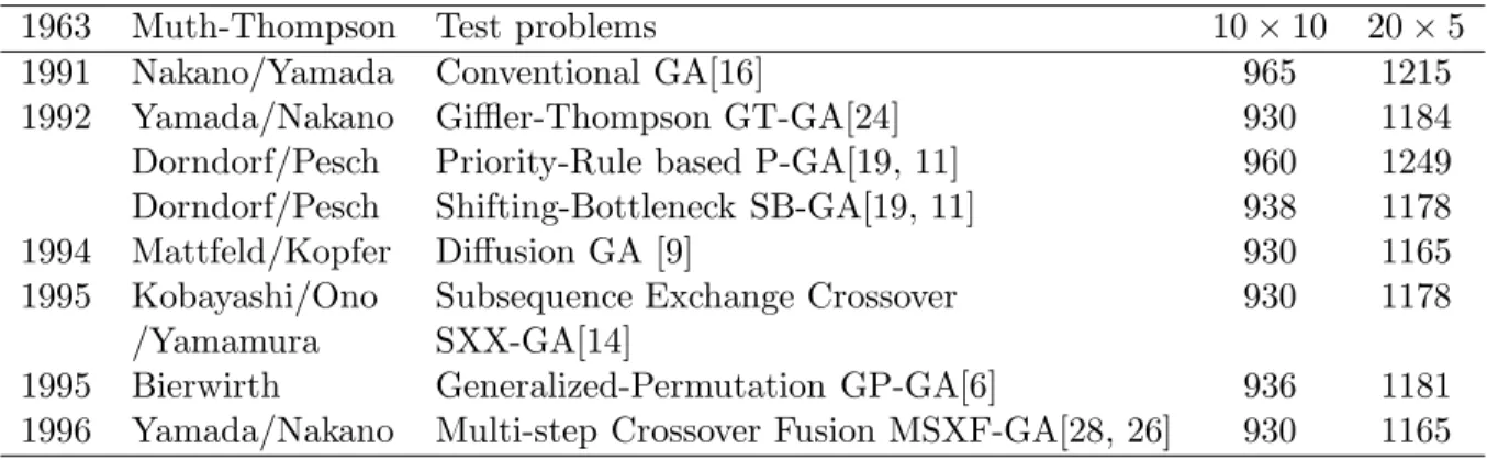
Table 2 summarizes the makespan performance of the methods described in this paper. This table is partially cited from [6]. The Conventional GA has only limited success and is outdated. It would be improved by being combined with the GT algorithm and/or the schedule reversal. The other results excluding the MSXF-GA results are somewhat similar to each other, although the SXX-GA is improved over the GT-GA in terms of speed and the number of times needed to find optimal solutions for the mt10 problem. The SB-GA produces better results using the very efficient and tailored shifting bottleneck procedure. The MSXF-GA which combines a GA and local search obtains the best results.
For the MSXF-GA, the population size = 10, constant temperature c= 10, number of iterations for each MSXF = 1000, Pr = 0.1 and Pc = 0.5 are used. The MSXF-GA
Table 2: Performance comparison using the MT benchmark problems
1963 Muth-Thompson Test problems 10×10 20×5
1991 Nakano/Yamada Conventional GA[16] 965 1215
1992 Yamada/Nakano Giffler-Thompson GT-GA[24] 930 1184
Dorndorf/Pesch Priority-Rule based P-GA[19, 11] 960 1249
Dorndorf/Pesch Shifting-Bottleneck SB-GA[19, 11] 938 1178
1994 Mattfeld/Kopfer Diffusion GA [9] 930 1165
1995 Kobayashi/Ono Subsequence Exchange Crossover 930 1178
/Yamamura SXX-GA[14]
1995 Bierwirth Generalized-Permutation GP-GA[6] 936 1181
1996 Yamada/Nakano Multi-step Crossover Fusion MSXF-GA[28, 26] 930 1165
in the C language. The MSXF-GA finds the optimal solutions for the mt10 and mt20 problems almost every time in less than five minutes on average.
7.2
The ten tough benchmark problems
Table 3 shows the makespan performance statistics of the MSXF-GA for the ten difficult benchmark problems proposed in [4]. The parameters used here were the same as those for the MT benchmark except for the population size = 20. The algorithm was terminated when an optimal solution was found or after 40 minutes of cpu time passed on the DEC Alpha 600 5/266. In the table, the column named lb shows the known lower bound or known optimal value (for la40) of the makespan, and the columns named bst, avg, var and wst show the best, average, variance and worst makespan values obtained, over 30 runs respectively. The columns namednoptand topt show the number of runs in which the
optimal schedules are obtained and their average cpu times in seconds. The problem data and lower bounds are taken from the OR-library [5]. Optimal solutions were found for half of the ten problems, and four of them were found very quickly. The small variances in the solution qualities indicate the stability of the MSXF-GA as an approximation method.
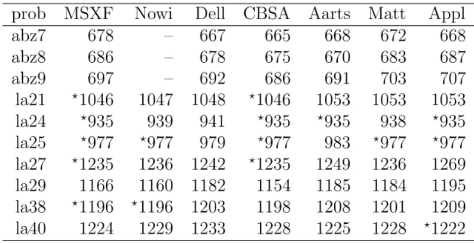
Table 4 shows comparison with various heuristic methods. In the table, MSXF rep-resents MSXF-GA method proposed in[28, 26], Nowi and Dell are tabu search methods proposed in [17] and [10] respectively, CBSA and Aarts are SA methods in [27] and [1]. Matt is the diffusion GA in [9], and Appl is from [4].
8
Conclusions
The first serious application of GAs to solve the JSSP was proposed by Nakano and Yamada using a bit string representation and conventional genetic operators. Although this approach is simple and straightforward, it is not very powerful. The idea to use the GT algorithm as a basic schedule builder was first proposed by Yamada and Nakano [24] and by Dorndorf and Pesch [11, 19] independently. The approaches by both groups and other active schedule-based GAs are suitable for middle-size problems; however, it seems necessary to combine each with other heuristics such as the shifting bottleneck or local search to solve larger-size problems.
Table 3: Results of the 10 tough problems prob size lb bst avg var wst nopt topt
abz7 20×15 655 678 692.5 0.94 703 – – abz8 20×15 638 686 703.1 1.54 724 – – abz9 20×15 656 697 719.6 1.53 732 – –
la21 15×10 – ⋆1046 1049.9 0.57 1055 9 687.7
la24 15×10 – ⋆935 938.8 0.34 941 4 864.1
la25 20×10 – ⋆977 979.6 0.40 984 9 765.6
la27 20×10 – ⋆1235 1253.6 1.56 1269 1 2364.75
la29 20×10 1130 1166 1181.9 1.31 1195 – – la38 15×15 – ⋆1196 1198.4 0.71 1208 21 1051.3
la40 15×15 ⋆1222 1224 1227.9 0.43 1233 – –
Table 4: Comparison with various heuristic methods on the 10 tough problems prob MSXF Nowi Dell CBSA Aarts Matt Appl
abz7 678 – 667 665 668 672 668
abz8 686 – 678 675 670 683 687
abz9 697 – 692 686 691 703 707
la21 ⋆1046 1047 1048 ⋆1046 1053 1053 1053
la24 ⋆935 939 941 ⋆935 ⋆935 938 ⋆935
la25 ⋆977 ⋆977 979 ⋆977 983 ⋆977 ⋆977
la27 ⋆1235 1236 1242 ⋆1235 1249 1236 1269
la29 1166 1160 1182 1154 1185 1184 1195 la38 ⋆1196 ⋆1196 1203 1198 1208 1201 1209
la40 1224 1229 1233 1228 1225 1228 ⋆1222
methods that use domain specific knowledge. The multi-step crossover fusion (MSXF) was proposed by Yamada and Nakano as a unified operator of a local search method and a recombination operator in genetic local search. The MSXF-GA outperforms other GA methods in terms of the MT benchmark and is able to find near-optimal solutions for the ten difficult benchmark problems, including optimal solutions for five of them.
References
[1] E.H.L. Aarts, P.J.M. van Laarhoven, J.K. Lenstra, and N.L.J. Ulder (1994). A computational study of local search algorithms for job shop scheduling. ORSA J. on Comput., 6(2):118–125.
[2] J. Adams, E. Balas, and D. Zawack (1988). The shifting bottleneck procedure for job shop scheduling. Mgmt. Sci., 34(3):391–401.
[3] D. Applegate (1992). Jobshop benchmark problem set. Personal Communication. [4] D. Applegate and W. Cook (1991). A computational study of the job-shop scheduling
[5] J.E. Beasley (1990). Or-library: distributing test problems by electronic mail. E. J. of Oper. Res., 41:1069–1072.
[6] C. Bierwirth (1995). A generalized permutation approach to job shop scheduling with genetic algorithms. OR Spektrum, 17:87–92.
[7] C. Bierwirth, D. Mattfeld, and H. Kopfer (1996). On permutation representations for scheduling problems. In 4th PPSN, pages 310–318.
[8] Y. Davidor, T. Yamada, and R. Nakano (1993). The ecological framework II: Im-proving GA performance at virtually zero cost. In5th ICGA, pages 171–176. [9] H. Kopfer D.C. Mattfeld and C. Bierwirth (1994). Control of parallel population
dynamics by social-like behavior of GA-individuals. In 3rd PPSN.
[10] M. Dell’Amico and M. Trubian (1993). Applying tabu search to the job-shop schedul-ing problem. Annals of Operations Research, 41:231–252.
[11] U. Dorndorf and E. Pesch (1995). Evolution based learning in a job shop scheduling environment. Computers Ops Res, 22:25–40.
[12] B. Giffler and G.L. Thompson (1960). Algorithms for solving production scheduling problems. Oper. Res., 8:487–503.
[13] M. Kobayashi, T. Ono, and S. Kobayashi (1992). Character-preserving genetic al-gorithms for traveling salesman problem (in japanese). Journal of Japanese Society for Artificial Intelligence, 7:1049–1059.
[14] S. Kobayashi, I. Ono, and M. Yamamura (1995). An efficient genetic algorithm for job shop scheduling problems. In 6th ICGA, pages 506–511.
[15] J.F. Muth and G.L. Thompson (1963). Industrial Scheduling. Prentice-Hall, Engle-wood Cliffs, N.J..
[16] R. Nakano and T. Yamada (1991). Conventional genetic algorithm for job shop problems. In 4th ICGA, pages 474–479.
[17] E. Nowicki and C. Smutnicki (1993). A fast taboo search algorithm for the job shop problem. Institute of Engineering Cybernetics, Technical University of Wroclaw, Wroclaw, Poland., Preprinty nr 8/93.
[18] S. S. Panwalkar and Wafix Iskander (1977). A survey of scheduling rules. Oper. Res., 25(1):45–61.
[19] E. Pesch (1994). Learning in Automated manufacturing: a local search approach. Physica-Verlag, Heidelberg, Germany.
[20] C. R. Reeves (1994). Genetic algorithms and neighbourhood search. InEvolutionary Computing, AISB Workshop (Leeds, U.K.), pages 115–130.
[22] N.L.J. Ulder, E. Pesch, P.J.M. van Laarhoven, J. Bandelt, H, and E.H.L. Aarts (1994). Genetic local search algorithm for the traveling salesman problem. In 1st PPSN, pages 109–116.
[23] D. Whitley (1989). The genitor algorithm and selection pressure: why rank-based allocation of reproductive trials is best. In 3rd ICGA, pages 116–121.
[24] T. Yamada and R. Nakano (1992). A genetic algorithm applicable to large-scale job-shop problems. In 2nd PPSN, pages 281–290.
[25] T. Yamada and R. Nakano (1995). A genetic algorithm with multi-step crossover for job-shop scheduling problems. In GALESIA ’95, pages 146–151.
[26] T. Yamada and R. Nakano (1996). A fusion of crossover and local search. InIEEE International Conference on Industrial Technology (ICIT ’96).
[27] T. Yamada and R. Nakano (1996). Job-Shop Scheduling by Simulated Annealing Combined with Deterministic Local Search. pages 237–248, Kluwer academic pub-lishers, MA, USA.