An Improved Population Migration Algorithm
Introducing the Local Search Mechanism of the
Leap-Frog Algorithm and Crossover Operator
Yanqing Zhang, Xueying Liu*
Department of Mathematics, Inner Mongolia University of Technology, Hohhot, China
Abstract
The population migration algorithm (PMA) is a simulation of a population of the intelligent algorithm. Given the prematurity and low precision of PMA, this paper introduces a local search mechanism of the leap-frog algorithm and crossover operator to improve the PMA search speed and global convergence properties. The typical test function verifies the improved algorithm through its performance. Compared with the improved population migration and other intelligential algorithms, the result shows that the convergence rate of the improved PMA is very high and its convergence is proved.
Citation:Zhang Y, Liu X (2013) An Improved Population Migration Algorithm Introducing the Local Search Mechanism of the Leap-Frog Algorithm and Crossover Operator. PLoS ONE 8(2): e56652. doi:10.1371/journal.pone.0056652
Editor:Vladimir Brusic, Dana-Farber Cancer Institute, United States of America ReceivedNovember 2, 2012;AcceptedJanuary 11, 2013;PublishedFebruary 2 , 2013
Copyright:ß2013 Zhang, Liu. This is an open-access article distributed under the terms of the Creative Commons Attribution License, which permits unrestricted use, distribution, and reproduction in any medium, provided the original author and source are credited.
Funding:This work was supported by the Scientific Research Project of the Higher Education Institutions of Inner Mongolia Autonomous Region No. NJZY12070. The funders had no role in study design, data collection and analysis, decision to publish, or preparation of the manuscript.
Competing Interests:The authors have declared that no competing interests exist. * E-mail: [email protected]
Introduction
The population migration algorithm (PMA) was proposed by Zhou et al in 2003 [1–2]. The PMA is a simulated population migration theory global optimization algorithm. The PMA is also a simulated mechanism that involves population along with economic center transfer and population pressure diffusion in the field. In other words, people relocate to a preferential region that has a high level of economic development and employment opportunities. When the preferential region has relative overpop-ulation, the population pressure constantly increases. When population pressure exceeds a certain limit, people will move to a more suitable preferential region. Population pressure makes the PMA engage in a better regional search. To a certain extent, population proliferation can prevent the PMA from falling into a local optimal solution. The whole algorithm shows alternate features that localized search and scatter search have in the search process.
In 2004, Xu gave an improved PMA (IPMA), which can be summarized into three forms: population flow, population migration, and population proliferation [3]. Population flow states that the population residing in the region is spontaneous and the overall flow is uncertain. Population migration is based on the mechanism across a wide range of the selection movement, in which people flow to the rich place. When the population pressure is very high, population proliferation is a selective movement from a preferential area to a no preferential area. It also reflects the people’s pioneering spirit.
Recent, various kinds of intelligent algorithms have been improved by many researchers. Wang et al improved the PMA with the steepest descent operator and the Gauss mutation [4]. Ouyang et al introduced the simplex in the PMA to improve the search performance of the algorithm [5]. Guo et al increased
performance of the population migration by improving the migrations’ efficiency [6]. Karaboga improved the bee swarm [7]. Li et al introduced extremal optimization to improve the performance of the shuffled frog leaping algorithm (SFLA) [8]. However, the results of all these studies show low accuracy or fall into the local optimal solution. To further improve the local search ability of the PMA and speed up convergence, we introduce a local search mechanism of frog leaping and crossover. This paper is improved and uses a number of classic functions for the simulation to show that the algorithm is effective and feasible.
Population Migration Algorithm
Consider the following unconstrained single-objective optimi-zation problem:
min f (X) ð1Þ
s:t X[S
In which f :S?R1 is a real valued mapping, X[Rn,
S~Pn
i~1½ai,biis a search space,aivbi. We assume that problem
(1) has a constant solution, namely, global optimal solution exists and the setHof the global optimal solution is not empty. Seeking the most value problem can be transformed into the form of problem (1). In the algorithm,Xis an individual and stands for the population and various kinds of information.Xi~(Xi
1,X2i,:::,Xni)is
the ith individual in the solution space, Xi[Rn; Xi
jis the ith
individual of thejthweight;di[Rn, di
j is thejthweight of theith
stands for population size. Target functionf(x) corresponds to the population attraction. The optimal solution (a local optimal solution) of problem (1) corresponds to the most attractive region (the preferential). The ability of the PMA to escape from the local optimal solution corresponds to the ability. Due to population pressure increase, the population moves out of the preferential area. The rise of algorithm or mountain climbing made the populations move into the preferential area. Local random search of algorithm corresponds to the population flow. The method by which the algorithm selects the approximate solution corresponds to the population migration. Escaping from the local optimal strategies corresponds to the population proliferation.
Frog Leaping Algorithm of Local Search
SFLA is proposed, as proved by Eusuff in 2003 [9]. SFLA is based on the heuristic and collaborative search of species. The implementation of the algorithm simulates the element evolution behavior of nature.
The implementation process of SFLA simulates the feeding behavior of a group of frogs in a wetland [10]. In the feeding process, every frog can be seen as the carrier of ideas and information. Frogs can communicate through the exchange of information, which can improve the knowledge of others. Every frog represents a solution to the optimization problem (1). Wetland represents the solution space. In the algorithm implemental stage, there areFfrogs divided into Ngroups. Each group haslfrogs. Different groups have different ideas and information. In a group, frogs follow the element evolution strategy in the solution space for local depth search and internal communication.
S~rand()(Pbi{Pwi) ð2Þ
P1wi~PwizS ð3Þ
In the above formulas, rand() is a random function that randomly generates the value in the range [0,1],Sis a step of the frog leaping, Pwi stands for the worst frog of the ith group, Pbi stands for the best frog of the ithgroup, and P1wistands for an update of the worst frog of theithgroup. If the adaptive value of the updated worst frog is more than that of the original worst frog in the same group, the updated worst frog will replace the original worst frog. Otherwise, a frog will be randomly generated in the group instead of the original worst frog. The updated process is repeated until the predetermined number of local searchLS. When all groups have completed the depth of local search, all the frogs of the groups are again mixed and divided into N groups. We continue the local search in the groups until the termination rule holds true, and then we stop.
Crossover Operators
By two leaner combinations, we can obtain two new individuals. Arithmetic crossover operation is often used to express individuals by floating individual coding. Hypothesis: The two parents are Xa~(X11,X21,:::,Xn1)andXb~(X12,X22,:::,Xn2).
Then,n random numbers are randomly generated, in which ai[(0,1), i~1,2,:::,n. After hybrid implementation, two new
progenies are generated:
Ya~(Y11,Y21,:::,Yn1),Yb~(Y12,Y22,:::,Yn2)
Yi1~aiXi1z(1{a)Xi2,Yi2~aiXi2z(1{ai)Xi1,i~1,2,::,n:
Methods
In the PMA, the population flow includes extensive information exchange. In practice, population information exchange decides the direction of the migration under certain conditions, so we should give full attention to population flow. When under pressure, population migration is the random population flow in the range of the population pressure, which does not have a significant role in further improving the algorithm.
The local search mechanism of frog-leaping algorithm and the crossover operator are introduced into the PMA in the process of population flow, which can well improve the original search results. IMPA organically made the frog-leaping combine with the crossover operator in the PMA. The process of the algorithm is as follows:
Initialization
Input the population sizeN, the initial radiusd(0), the vigilance parameter of population pressure a(0), the number of the population flow l, the number of local search LS, and the
maximum number of iterations T. We randomly generate N
individuals in the search spaceS,X1,X2, …,XN. Theithregional
center centeri~Xi determines the upper and lower
centeri+dibounds of the ith region, in which , di jw0,
i~1,2,:::,N,j~1,:::,n.The extraction methoddij makesdi equal, so we cancel the superscript ofdiin the following steps. We obtain an initial search spaceV(0)~S
N i~1
B(X(i)(0),d(0)), which stands for
the initial residential area. The setB(X,d)is taken as the sphere, in whichXis the center andris the radium. The following variables appearing that way are the same. f(X0)~max
1ƒiƒ(X
i) and
Xbest(0)~X0. We set iteration countert= 0.
Evolutionary
1. Preparation:g(t)~d(t)
2. Population flow: In every B(X(i)(t),g(t)), we randomly
generateliindividuals, so we can obtain the groupY(t) inV(t), which hasNlindividuals.
3. Population migration
We next introduce the local search mechanism of frog-leaping algorithm and crossover operator. At this time, the role of population has been transformed to the frog. The search area is seen as the frog’s wetland. The formedNlocal areas are seen as the
Ngroups. The individual of every local area is seen as the frog.
(a) We choose N best frogs in Y(t), which form the intermediate frog groupYbest(t)~fYbest(1)(t),Y
(2)
best(t),:::,Y
(N)
bestg.
(b) FormingNregions:fB(Ybest(i) (t),g(t)),i~1,2,:::,Ng. (c) In every group, we produce a frog body flow. In other words,liindividuals are randomly generated inB(Ybest(i) (t),g(t)).
liand the adaptive value ofYbest(i) are proportional.
(e) In theiNthgroup, we calculate the adaptive value of every frog in the group and arrange them in descending order. We can obtain the best solutionPbiand the worst solutionPwi.
(f)Phwi=Pwi, according to the following four formulas, we can update and improve the position of the worst frog in the group.
S~rand()(Pbi{Pwi) ð4Þ
P1wi~PwizS,{SmaxƒSƒSmax ð5Þ
e~rand() ð6Þ
newPwi~eP1wiz(1{e)Phwi ð7Þ
(g) If step (f) improved the position of the worst frog, the adaptive value ofnewPwiis more than thePwi’s, the position of
Pwi will be replaced by the position of newPwi.That is,
Pwi~newPwi. Otherwise, we randomly generate a position of
a frog instead of the worst frog in the group.
(h) Ifim,LS, thenim=im+1and turn to step (f). Otherwise, we report the best frogZbest(i) (t)and turn to step (i).
(i) IfiN,N, theniN=iN+1 and we turn to step (e). Otherwise, we turn to step (j).
(j) Contraction of preferential region:g(t)~(1{D)g(t), (0vDv1).
(k) Ifg(t)wa(t)(not more than the population pressure alert), we continue the frog flow and turn to step (c) Otherwise, we turn to step (l).
(l) We report N the best frogs:Zbest(t)~fZbest1 (t),
Z2
best(t),:::,ZNbest(t)g.
4. Population proliferation:
(a) We keep the best individual in theZbest, which is credited
asZ0
best.
(b) In the V(t), we randomly sample N-1 new individuals instead of theN-1 individuals offZbest(t)\Z0bestg.
(c) We define a new generation of population
X(tz1)~fX1(tz1),X2(tz1),:::,XN{1(tz1),Z0
best(t)g:
Termination of Inspection
If the new generation of populationX(t+1) contains the eligible solution, we stop and output the best solution inX(t+1). Otherwise, we narrowd(t)and a(t)properly and sett:t+1. If the maximum numbers of iterations for the algorithm are not met, we turn to the second step.
Convergence Analysis
This paper uses the axiom model to analyze and prove the convergence of IMPA.
Definition 1 Optimization variables X have limited-length
characters and have the formA~a1a2:::an[X~(x1,x2:::xn).nis
called the code string length ofX,Ais called the code ofX, andXis called the decode of the character A. ai is considered a genetic
gene. All possible values of ai are called allelic gene. A is a chromosome made up ofngenes [11].
Definition 2(Individual Space)Cis an allelic gene.nis given
the code string length. The setHl~fa1a2:::an,ai[C,i~1,2,:::,ng
is called individual, in which VN is a natural number and HN~HH:::H
|fflfflfflfflfflfflfflfflfflfflffl{zfflfflfflfflfflfflfflfflfflfflffl}
N
is theNorder of population space [11].
Definition 3 (Satisfaction Set) If VX[B,Y=[B, then
f(X)wf(Y). B(X) is called the satisfaction set. The number of individuals in the setB(X) is used forDB(X)D.XX[HN
n is any of the
population and Xb is the best individual in the set XX. The
satisfaction set induced by Xbis called satisfaction set of the
populationXX, which is marked Bb(XX)~fX[Hl,f(X)§f(XX)g. All
of the satisfaction sets’ intersections are formed with the global optimal solutionB[11].
Definition 4(Selection Operator) The selection operatorSis a
random mapping, S:HNl?HN. It meets the following two
conditions. (1) ForVXX[HN
n, we can obtain½SXXi[XX,i~1,2,:::,N,
in which½SXXi stands for the iindividual in the SXX; (2) Any
population XXthat meets DB(XX)DvNhas PfDB(SXX)Dz (N{M)wDB(XX)Dgw0. The first condition states that selected individuals should be in the selected population. The second condition states that the selection operator may increase the number of optimal individuals in the population, in addition to variations of the individuals’ numbers between selected population and original population [11].
Definition 5(Reproduction Operator) Reproduction operator
Ris a random mapping.R:HN?HNl. If any populationXX[HN n,
which meetsPfR(XX)\Bb(XX)=Wgw0, the new populationR(XX)
whichXXbecomes under the action of the operatorR, may contain
more satisfied individuals than the original population [11].
Definition 6(Mutation Operator) Mutation operator Mis a
random mapping: M:HNl
l ?HlNl.VXX[HnNmeetsPfM(XX)\
B=Wgw0. Mutation operator is the reproduction operator that has a much better nature. If the population contains satisfied individuals, then after mutation, the population should contain satisfied individuals. If the population does not have satisfied individuals, then after mutation, the population may contain satisfied individuals [11].
In improved population migration, extended operator
L0:HlN?HlNl meets the following expressions:
L0(X)~(X(1),:::,X(1) |fflfflfflfflfflfflfflffl{zfflfflfflfflfflfflfflffl}
l
,:::,X(N),:::,X(N)
|fflfflfflfflfflfflfflfflffl{zfflfflfflfflfflfflfflfflffl}
l
),
HN
l ~HlHl:::Hl
|fflfflfflfflfflfflfflfflfflfflfflfflffl{zfflfflfflfflfflfflfflfflfflfflfflfflffl}
N
and
VX~(X(1),X(2),:::,X(N))[HlN:
Uniform mutation operatorMt:HlNl?HlNl,
VY~(Y(1),Y(2),:::,Y(N))[HnNl,Mt(Y)
~(Mt(Y(1)),Mt(Y(2)),:::,Mt(Y(Nl))):
Therefore, we can use the operatorMtL0:HlN?HlNl to stand
for the process of step (a) in population migration, where we chose
N, the best individuals from population Y(t). The reproduction operatorR1stands for the progress from step (b) to the process of final outputZbest(t) in step (l). The reproduction operatorR2stands for the process from population proliferation to finally generate
X(t+1). Therefore, the IPMA can be expressed as:
X(tz1)~R2R1S1MtL0(X(t)),t~0,1,2,::: ð8Þ
Y(t)~MtL(X(t)),S~S1,R~MtL0R2R1,t~1,2,::: ð9Þ
After both sides have the same function of operatorMtL0for
(8), we can find thatY(tz1)~RS(Y(t)).The general simulated evolution algorithm can be composed of a series of selection operatorsf gSt and reproduction operatorsf gRt to be represented
abstractly as follows:X(tz1)~RtSt(X(t)).
Lemma 1In the IPMA,S is a selection operator andR is a
reproduction operator. The proof can be obtained from reference [11].
Theorem 1The IPMA is a simulated evolutionary algorithm.
Lemma 2 In the IPMA, the characteristic number of the
preferred selection operator, the selection pressure of the operator
S:PS= 1, the selection intensity aS= 1. The IPMA just takes the preferred selection operator. According to reference [3], the selection pressure and the selection intensity are defined to calculate the characteristic number of the operator S. The proof can be obtained from reference [11].
Lemma 3 In the IPMA, the characteristic number of the
reproduction operator, the operator R:HN l ?HNl
zN
l , then the
absorption and scattering rate of the reproduction meet the following estimates: AE§Nlrbt(1r(z1)
z1)1((e))½1b((e) z1)
1 ,
Sk
R~0. Where, e~C(e)d(dis the radius of the search space) is
the radius of the set of optimal solutionBandbtis a conversion coefficient. If the set Bincludes a division region in theV(z1), thenbt~1; otherwise,btis the rate of volume of the intersection of the set Band a division region. Thus, we can obtain 0ƒbtƒ1. The proof can be obtained from reference [11].
Lemma 4 If the abstract simulated evolutionary algorithm
(SEA) satisfies the following conditions: (1) the pressure of selection operator f gSt is uniformly bounded; (2) the absorption of
reproduction operatorf gRt : Ae(t)
meets P
?
t~1
E(t)~?; (3) the
strength of selection as(t)
, absorption Ae(t)
, and scattering Sm0
e(t) n o
content are as follows: lim
t??½1-(1-S
m0
R(t))as(t)=AR(t)~0.
Then, an abstract and a general SEA will probably weakly approach the optimal solution set. The proof can be obtained from reference [11].
Theorem 2(Convergence of IPMA) If the IPMA adopts the
selection operator family ftg, which comprise all the preferred
selection operators, reproduction operators familyftg, in which
Y(tz1)~RS(Y(t)). The following conditions are thus met: (1); (2)bt~O(1=)(bt~O((Ctz1)n)).
Then, to prove that the IPMA will probably weakly approach the solution set, the following steps are performed.
Proving. Known by lemma 2: Ps(t)~1,as(t)~1; Known by
lemma 3: AE§Nlrbt(1-r(Ctz1)n
z1)N-1(C(e)n)½1 -bt(
C(e)
Ctz1)
nl-1~ O(1=t),Sk
R~0; wheneis given,C(e)is also given. By condition (1),
we obtain lim
t??r((Ctz1)
nz1)N-1~1. By condition (2), we obtain
bt~O((Ctz1)n), then lim
t??½1-bt(C(e)=Ctz1)
n
l-1=0. We have
bt~O(1=t) and lemma 3, then AE§Nlrbt(1-r(Ctz1)n
z1)N-1
(C(e)n)½1-bt(CCt(ze)1)
nl-1~O(1=t). We know the divergence of the harmonic series, so P
?
t~1
AR(t)~?. According to lemma 3:SR1~0.
According to lemma 2:as(t)~1, solim
t??(1-(1-S
1
R(t))as(t))=AR(t)~0.
The three conditions of lemma 3 are met. The IPMA probably weakly approaches the global optimal solution.
Results and Discussion
Simulation Examples and Experimental Parameter Setting
To verify the performance of the IPMA, this paper performs an experiment. The IPMA is compared with the basic population algorithm and other improved algorithms. In the simulation experiment, we choose 10 classic test functions to test the algorithm. According to the performance of the functions, they are divided into a single minimum (single) and a number of local minima (multimodal) into two categories. The following lists the 10 functions’ definition, variable range, and global optimal values of the theory and optimal solution of the theory. The functionf1is a unimodal function used to examine the accuracy of the algorithm. The functionf2which contains infinite local optimal solution and has infinite local maximum near suboptimal solution, is a strong shock multimodal function. General optimization algorithms easily fall into local optimal solution. Thus, the ability of the algorithm is used to avoid falling into a local optimization algorithm. The function f5 is a multimodal function. It has about 10*D (D is dimension) local optimal solution. The functionf6 is a deep and local minimum multimodal function that has many local optimal solutions. The functionsf5andf7are complex nonlinears used to test global search performance of algorithms. The functionf8is a complex and classical function used to test the optimization efficiency of algorithms. In a certain number of iterations, this paper estimates the performance of IMPM by the test function of the best value, the worst value, average value, variance, average running time, and convergence rate.
1. Sphere Model function: minf1~P
n i~1
X2
i,DXiDƒ100. The
optimal solution is (X1,X2,:::,Xn)~(0,0,:::,0) and the optimal
minimum value is 0, whenn= 30.
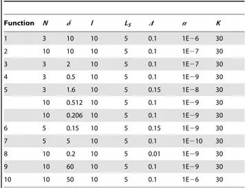
Table 1.Parameter setting of the functions for the IPMA.
Function N d l LS D a K
1 3 10 10 5 0.1 1E26 30
2 10 10 10 5 0.1 1E27 30
3 3 2 10 5 0.1 1E27 30
4 3 0.5 10 5 0.1 1E29 30
5 3 1.6 10 5 0.15 1E28 30
10 0.512 10 5 0.1 1E29 30
10 0.206 10 5 0.1 1E29 30
6 5 0.15 10 5 0.15 1E29 30
7 5 5 10 5 0.1 1E210 30
8 10 0.2 10 5 0.01 1E29 30
9 10 60 10 5 0.1 1E29 30
10 10 50 10 5 0.1 1E26 30
2. Schaffer function: maxf2~0:5{
sin2( ffiffiffiffiffiffiffiffiffiffiffiffiX2 1zX
2 2 p
){0:5 ½1:0z0:001(X2
1zX22) 2,
{100ƒXiƒ100,i= 1,2. The optimal solution is (X1,X2) = (0, 0) and the optimal maximum value is 1.
3. minf3~P 5
i~1
interger(Xi), {5:12ƒXiƒ5:12, i~1,2,:::,5.
The function in the section (25.12, 25) has a global minimum value230.
4. minf4~{5 sinX1sinX2sinX3sinX4sinX5{sin (5X1) sin (5X2) sin (5X3) sin (5X4) sin (5X5), 0ƒXiƒp, i~1,2,:::,5.
The optimal solution is(X1,X2,:::,X5)~(p=2,p=2,:::,p=2)and the
optimal minimum value is26.
5. Generalized Rastrigin function: . The function has many local minimum solutions, but it has only one global minimum
solution (X1,X2) = (0, 0) and the global minimum value is 0, when
n= 2,n= 5 andn= 10.
6. Quartic function: minf6~P
n i~1
iX2
i,{100ƒXiƒ100,
i~1,2,:::,n:. The optimal solution is (X1,X2,:::,X5)~(0,0,:::,0)
and the optimal minimum value is 0, whenn= 20. 7. Ackley’s function: minf7~{20 exp½{0:2
ffiffiffiffiffiffiffiffiffiffiffiffiffiffiffiffiffiffi Pn
i~1
X2 i=n s
{ exp (P
n i~1
cos ((2pXi)=n))z20{e, DXiDƒ32. The optimal solution
is(X1,X2,:::,Xn)~(0,0,:::,0)and the optimal minimum value is 0,
whenn= 20.
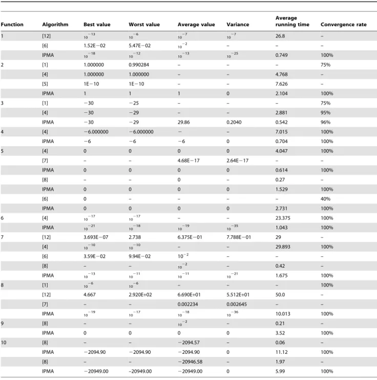
8. Generalized Rosen Brock’s function: Table 2.Comparison performance of the IPMA in the ten functions.
Function Algorithm Best value Worst value Average value Variance
Average
running time Convergence rate
1 [12] 10213 1026 1027 1027 26.8 –
[6] 1.52E202 5.47E202 1022 – – –
IPMA 10218 10212 10213 10225 0.749 100%
2 [1] 1.000000 0.990284 – – – 75%
[4] 1.000000 1.000000 – – 4.768 –
[5] 1E210 1E210 – – 7.626 –
IPMA 1 1 1 0 2.104 100%
3 [1] 230 225 – – – 75%
[4] 230 229 – – 2.881 95%
IPMA 230 229 29.86 0.2040 0.542 96%
4 [4] 26.000000 26.000000 2 – 7.015 100%
IPMA 26 26 26 0 0.704 100%
5 [4] 0 0 0 0 4.047 100%
[7] – – 4.68E217 2.64E217 – –
IPMA 0 0 0 0 0.614 100%
[8] – – 0 – 0.27 –
IPMA 0 0 0 0 1.529 100%
[6] 0 – – – – 40%
IPMA 0 0 0 0 2.731 100%
6 [4] 10217 10217 – – 23.375 100%
IPMA 10221 10218 10219 10235 1.043 100%
7 [12] 3.693E207 2.738 6.375E201 7.788E201 29 –
[4] 10210 10210 – – 29.893 100%
[6] 3.59E202 9.94E202 1022 – – –
[8] – – 1022 – 0.42 –
IPMA 10213 10211 10211 10221 1.675 100%
8 [1] 1026 1026 – – – 100%
[12] 4.667 2.920E+02 6.690E+01 5.512E+01 50.0 –
[7] – – 0.002234 0.002645 – –
IPMA 10219 10217 10218 10236 10.013 100%
9 [8] – – 1022 – 0.21 –
IPMA 0 0 0 0 3.52 100%
10 [8] – – 22094.57 – 0.06 –
IPMA 22094.90 22094.90 22094.90 0 11.12 100%
[8] – – 220946.58 – 1.97 –
IPMA 220949.00 –20949.00 220949.00 0 5.99 100%
minf8~P
n{1
i~1½
100(Xiz1{Xi2)
2z(1{X
i)2,DXiDƒ2:048. The
optimal solution is (X1,X2,:::,Xn)~(1,1,:::,1) and the optimal
minimum value is 0, whenn= 3.
9. Griewank function:minf9~1=4000P
n i~1
X2
i-P
n
i~1cos (Xi= ffiffi
i p
)
z1,Xi[(-600,600). The optimal minimum value is 0, whenn= 30. 10. Schwefel function: minf10~-P
n i~1
Xisin ffiffiffiffiffiffiffiDXiD
p
,Xi[(-500,
500). The optimal minimum value is22094.9, whenn= 5. The optimal minimum value is220949, whenn= 50.
To verify the performance of the IPMA, we choose a computer whose CPU is made by AMD and has an operating system of Windows 7. The mathematical software Matlab7.0 was used for the testing. Each function is applied 50 times. We present the parameters in the process of solving the functions for this paper in the table 1. To show the better performance of the IPMA, we compare it with other algorithms through the following indicators: best and worst solutions, average solution, variance, average running time, and average convergence rate in 50 cycles.
This table shows parameter setting of the ten functions. Population size N, number of population flow l, radius d, coefficient of contraction D, pressure of population parameters
a, number of local searchLS, and largest number of iterationsK. li~l,dj(0)~(bi-ai)=2N.
Experimental Result and Analysis
In Table 2, the data of functionf1 show that the improved population algorithm is better than frog-leaping algorithm in terms of precision. Other algorithms find it very difficult to achieve the optimal solution of function f2, but the IPMA can easily do so,
which indicates that the algorithm’s ability of escaping from local optimal solution is very ideal. Function f8 can test whether the algorithm’s ability of global optimization is good. It is used to measure the efficiency of the algorithm, so we know the efficiency of the IPMA is very high compared with other algorithms from the data of functionf8.The data functionsf3,f4,f5,f7,f9andf10reflect that the IPMA is a better algorithm from a certain angle. Through cooperation of the best value, the worst value, the average value, the variance, and the convergence rate, the IPMA is found to be better than the other algorithms in the calculation of stability and precision.
Conclusions
In this paper, based on the local search mechanism and crossover operator, we put forward an IPMA. The parameters of the IPMA are simple and easy to realize. By testing the 10 functions, we find that the IPMA is better than the basic PMA and is superior to many intelligent algorithms. The PMA is good at global searches, but it does not perform well in local search and its precision is low. We introduce local search in population and crossover operator to improve these deficits. Therefore, the IPMA is increased to avoid falling into local optimum capacity; its calculation speed and precision are also improved.
Author Contributions
Conceived and designed the experiments: XYL. Performed the experi-ments: YQZ. Analyzed the data: YQZ XYL. Contributed reagents/ materials/analysis tools: YQZ. Wrote the paper: YQZ.
References
1. Zhou YH, Mao ZY (2003) A new search algorithm for global optimization: population migration algorithm (I). Journal of South China University of Technology (Nature Science) 31:1–5. (in Chinese).
2. Zhou YH, Mao ZY (2003) A new search algorithm for global optimization: population migration algorithm (II). Journal of South China University of Technology (Nature Science) 31: 41–43. (in Chinese).
3. Xu ZB (2004) Computational intelligence (Volume 1) - Simulated evolutionary computer. Beijing: High Education Press. 152p. (in Chinese).
4. Wang XH, Liu XY, Bai XH (2009) Population migration algorithm with Gauss mutation and steepest descent operator. Computer Engineering and Application 45: 57–60. (in Chinese).
5. Ouyang YJ, Zhang WW, Zhou YQ (2010) A based on the simplex and population migration hybrid global optimization algorithm. Computing Engineering and Application 46: 29–35. (in Chinese).
6. Guo YN, Cheng J, Cao YY (2011) A novel multi-population cultural algorithm adopting knowledge migration. Soft Computing 15: 897–905.
7. Karaboga D (2005) An idea based on honey bee swarm for numerical optimization. Technical Report-TR06, Erciyes University, Engineering Faculty, Computer Engineering Department. 10p.
8. Li X, Luo JP, Chen MR, Wang N (2012) An improved shuffled frog-leaping algorithm with extremal optimization for continuous optimization. Information Science 192: 143–151.
9. Eusuff MM, Lansey KE (2003) Optimization of water distribution network design using the shuffled frog leaping algorithm. Journal of Water Resource Planning and Management 129: 210–225.
10. Han Y, Cai JH (2010) Advances in Shuffled Frog Leaping algorithm. Computer Science 37: 16–19. (in Chinese).
11. Wu Y (2005) Convergence analysis on population migration algorithm. Xi’an: Xi’an University of science and Technology. 76p. (in Chinese).