doi: 10.1590/0101-7438.2018.038.03.0441
CHEMICAL REACTION OPTIMIZATION METAHEURISTIC FOR LOCATING SERVICE STATIONS THROUGH THE CAPACITATEDP-MEDIAN PROBLEM
Danilo C´esar Azeredo Silva* and M´ario Mestria
Received February 5, 2018 / Accepted July 13, 2018
ABSTRACT.Chemical Reaction Optimization (CRO) is a metaheuristic for solving optimization problems, which mimics the interactions between molecules in a chemical reaction with the purpose of achieving a stable, low-energy state. In the present work, we utilize the CRO metaheuristic to solve, in an efficient manner, the capacitatedp-median problem, in order to locate service stations. Results from solving small to medium-sized problems available in the literature, with up to 724 notes and 200 medians, are compared to their optimal or best-known values. Results show that CRO results are comparable, in terms of accuracy and execution time, to many existing successful metaheuristics, as well as exact and hybrid methods, having exceeding those in some cases.
Keywords: Chemical Reaction Optimization capacitatedp-median, metaheuristics.
1 INTRODUCTION
Facility layout and planning is an important topic that has a wide variety of applications in real life. Both private and public sectors are frequently faced with problems involving facility lay-out decisions. Facility location is concerned in finding the best locations for facilities based on supply-demand requirements. This problem has many applications in real life including locating retail stores, ambulance centers, schools, gas stations, electric vehicles charging stations, hospi-tals, fire stations, ATM machines, and wireless base stations. Design parameters of the facility location problem may include how many facilities should be sited, where should each facility be located, how large each facility should be, and how should demand be allocated.
Modeling of the facility location problem has been widely investigated in the literature. One of the best-known facility location models is the capacitated p-median problem (CPMP), which is a location problem where a set of objects (e.g., customers) has to be partitioned into a fixed number of disjoint clusters. Each object has an associated weight (or demand) and must be assigned to
*Corresponding author.
exactly one cluster. For a given cluster, the median is that object of the cluster from which the sum of the dissimilarities to all other objects in the cluster is minimized. The dissimilarity of a cluster is the sum of the dissimilarities between each object who belongs to the cluster and the median associated with the cluster. The dissimilarity is measured as a cost (e.g., distance) between any two customers. Each cluster has a given capacity, which must not be exceeded by the total weight of the customers in the cluster. The objective is to find a set of medians, which minimizes the total dissimilarity within each cluster.
The CPMP can be found in the literature under various different names, such as the capac-itated warehouse location problem, the sum-of-stars clustering problem, the capaccapac-itated clus-tering problem, and others. Another way to look at the problem is to consider it a variation of the classic p-median problem, which was first formulated by Hakimi (1964) and consists of locating p service stations to serve n customers, or nodes, in such a way that the average weighted distance between these customers and their closest stations is minimized. This model, which is also known as uncapacitated p-median problem, has been widely used to locate ser-vice stations and was proven, by Kariv & Hakimi (1979), to beNP-Hard. The CPMP extends the original p-median problem by adding a fixed demand to each customer. In addition, a ca-pacity restriction is added to each service station, so that the total demand from all customers, served by a given station, must not exceed its capacity. The CPMP is also known to beNP-Hard (Gary & Johnson 1979).
Mulvey & Beck (1984) were the first to extend the uncapacitated p-median problem, by adding a capacity constraint to each service station. In their seminal work, the authors propose a primal heuristic as well as a hybrid method, based on heuristic optimization and subgradients, to achieve good solutions for the problem. Since then, several other researchers have proposed approaches employing exact, heuristic or hybrid methods to provide good quality solutions to the problem, within acceptable computational times. Osman & Christofides (1994) developed a hybrid solu-tion, based on Simulated Annealing and Tabu Search metaheuristics, to provide near optimal to optimal solutions to a group of instances from 50 to 100 nodes and 5 to 10 medians. Maniezzo et al. (1998) presented an evolutionary method combined with an effective local search technique to solve a variety of CPMP problems, including the ones proposed by Osman & Christofides (1994). Baldacci et al. (2002) proposed an exact algorithm for solving the CPMP based on a set parti-tioning formulation. Lorena & Senne (2003) proposed a local search heuristic for the capacitated
p-median problem to be used in solutions made feasible by a Lagrangean/surrogate optimiza-tion process, which explores improvements on upper bounds limits of primal-dual heuristics, based on location-allocation procedures that swap medians and vertices inside clusters, real-locate vertices, and iterate until no improvements occur. The authors used instances from the literature as well as real data provided by a geographical information system. A version of a Genetic Algorithm was developed by Correa et al. (2004).
from a geographic database from the city of S˜ao Jos´e dos Campos, Brazil. Ahmadi & Osman (2005) proposed a metaheuristic called Greedy Random Adaptive Memory Programming Search (GRAMPS) for the capacitated clustering problem. A branch-and-price algorithm for the CPMP was proposed by Ceselli & Righini (2005). Scheuerer & Wendolsky (2006) proposed a scatter search heuristic for the capacitated clustering problem. It was evaluated on instances from the lit-erature, obtaining several new best solutions. Diaz & Fernandez (2006) proposed a hybrid scatter search and path relinking heuristic for the same problem. The authors ran a series of computa-tional experiments evaluating the proposed methods on instances from the literature, including instances corresponding to 737 cities in Spain. Chaves et al. (2007) presented a hybrid heuristic called Clustering search (CS), which consisted in detecting promising search areas based on clus-tering. Boccia et al. (2008) proposed a cut-and- branch approach, which proved to be effective in solving hard instances, using IBM CPLEX, or reducing their integrality gap. Fleszar & Hindi (2008) developed a hybrid heuristic that utilizes Variable Neighborhood Search to find suitable medians, thus reducing the CPMP to a generalized assignment problem, which was then solved using IBM CPLEX. Stefanello et al. (2015) presented a matheuristic approach, which consisted of reducing mathematical models by heuristic elimination of variables that are unlikely to be-long to a good or optimal solution. Additionally, a partial optimization algorithm based on their reduction technique was proposed. Resulting models were solved by IBM CPLEX, with good accuracy and performance.
Chemical Reaction Optimization (CRO) is a recently created metaheuristic for optimization, inspired by the nature of chemical reactions, proposed by Lam & Li (2012). A chemical reaction is a natural process of transforming unstable substances into stable ones. Under a microscopic view, a chemical reaction starts with some unstable molecules with excessive energy. These molecules interact with each other through a sequence of elementary reactions. At the end, they are converted to molecules with minimum energy to support their existence. This property is embedded in CRO to solve optimization problems.
CRO has been used to address a broad range of problems in both discrete and continuous do-mains. Lam & Li (2010) proposed a solution for the quadratic assignment problem, whereas Xu et al. (2010) implemented a parallelized version of CRO for the same problem. James et al. (2011) employed CRO to train artificial neural networks. Lam et al. (2012) extended CRO to solve continuous problems. Xu et al. (2011b) utilized it for stock portfolio selection. CRO was also used for solving task scheduling problems in grid computing by Xu et al. (2011a).
This paper is organized as follows: Section 2 provides a formal description of the CPMP for locating service stations. Section 3 describes the CRO metaheuristic, focusing on the customiza-tions that we implement to solve the CPMP, including a simple constructive heuristics and a
λ-interchange mechanism used during the local search phase. Section 4 contains the computa-tional results of our studies for all tested instances. Conclusions and future developments are presented in Section 5.
2 THE CPMP PROBLEM
The CPMP problem, depicted in this paper, aims to locate service stations, from a set of candidate locations and a set of customers. The CPMP integer linear programming model is shown below: Decision variables:
xj =1 if candidate station jwas selected; or 0, otherwise; (1)
yi j =1 if demand centeriis served by stationj;ou 0, otherwise; (2)
Model:
min i∈I
j∈J
di jyi j (3)
subject to:
j∈J
xj = p, ∀j∈ J (4)
j∈J
yi j =1, ∀i ∈I (5)
yi j−xj ≤0, ∀i ∈I, ∀j∈ J (6)
i∈I
Diyi j ≤cjxj, ∀j ∈ J (7)
xj ∈ {0,1}, ∀j ∈ J (8)
yi j ∈ {0,1}, ∀i ∈ I, ∀j ∈ J (9)
where:
J = set of candidate service station locations (median candidates);
I = set of customers (nodes);
di j = distance, or cost, from customerito service station j;
p = number of medians or stations to be opened;
Di = demand associated to customeri;
cj = capacity of service station j.
number of selected stations to be equal top, whereas, constraint (5) requires the demands from all customers to be met. Constraint (6) ensures that a customer is associated only to a service station that is selected. Constraint (7) makes sure that the total demand from all customers assigned to a station does not exceed its capacity. Finally, constraints (8) and (9) define the domain of the decision variablesxandy. Without loss of generality, we assume that J =I, in this paper.
3 CRO METHAHEURISTICS FOR THE CAPACITATEDP-MEDIAN PROBLEM
The CRO metaheuristic is a technique developed by Lam & Li (2012), which loosely relates chemical reactions with optimization and is based on the first two laws of thermodynamics. The first law, the conservation of energy, states that energy cannot be created or destroyed, but only transformed or transferred from one entity to another. The second law states that entropy, which is the measure of the degree of disorder of a system, tends to increase.
A chemical reaction system consists of the chemicals substances and their environment. The energy of the environment is symbolically represented by a central energy reservoir, i.e., a buffer. A chemical substance is comprised of molecules, which possess potential and kinetic energy. A chemical reaction occurs when the system is unstable, due to excessive energy. All chemical reaction systems tend to reach a balanced state, in which potential energy drops to a minimum. CRO simulates this phenomenon, by gradually converting potential energy into kinetic energy and transferring energy from the molecules to the environment through consecutive steps or sub-reactions, over several transition states, which result in compounds that are more stable and contain minimal energy. It is an iterative process that seeks the ideal point.
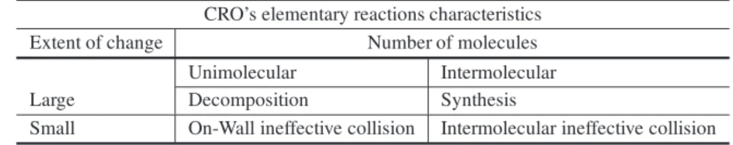
A collision provokes a chemical change in a molecule. There are two types of collisions in CRO: unimolecular and intermolecular. The first ones describes the situation in which a molecule collides with the wall of a container, whereas the latter represents the cases in which a molecule collides with other molecules. Such chemical change is called an elementary reaction. An ineffec-tive elemental reaction is one that results in a subtle change in molecular structure. CRO utilizes four types of elementary reactions: on-wall ineffective collision, decomposition, intermolecular ineffective collision and synthesis. Decompositions and syntheses cause much more vigorous changes in molecular structures. Elemental molecular reactions are summarized in Table 1.
Table 1–CRO’s elementary reactions. CRO’s elementary reactions characteristics
Extent of change Number of molecules
Unimolecular Intermolecular
Large Decomposition Synthesis
Small On-Wall ineffective collision Intermolecular ineffective collision
CRO is a variable population-based metaheuristic. Therefore, the number of molecules may change at each iteration. In ineffective collisions, the number of molecules remains the same. In decompositions, this number increases and in syntheses, it decreases. It is possible to influence the frequency of decomposition and synthesis, indirectly, by changing CRO’s parameters called
αandβ, respectively. Elementary reactions define how molecular reactions are implemented. In the present work, CRO is implemeted using C# object-oriented programming language, due to the easiness of modeling molecules as instances of a class which contains all the attributes needed for its operation. The molecule and elementary reactions, as well as the main algorithm for the CRO are implemented as methods of classes. The following subsections describe the main components of the CRO focusing on the modifications that are done to solve the CPMP. Further information about the CRO metaheuristics can be obtained in Lam & Li (2010, 2012).
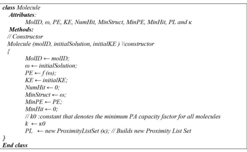
3.1 The Molecule
The basic unit of the CRO algorithm is the molecule, which contains several attributes that are essential to its proper operation. For this implementation of CRO, which we call CRO for the CPMP, we define the following attributes:
• Molecule ID (MolID): uniquely identifies a molecule in the population of molecules.
• Molecular structure(ω): stores a feasible solution for the problem, which is comprised of the objective function value, as well as the decision variablesx(1)and y(2). The x
decision variable set stores the current station selection for a given feasible solution. It is implemented as alist of integers, thus storing only the station numbers that are part of the solution. For instance, if the number of candidate stations is 100 and the number of medians is five,x will store five values corresponding to the currently selected stations, such as the list{5,17,29,45,79}. This has proven to be more effective than storing x
as an array of bits of size|J|. Similarly, the decision variable set y, which stores the customer-to-station assignments, is implemented as an array of integers of size|I|, instead of a matrix of bits of size|J| × |I|.
• Potential Energy (PE): it is defined as the objective function value in the molecular struc-ture(ω). If f denotes the objective function, thenP Eω= f(ω).
• Kinetic Energy (KE): it is a non-negative number that quantifies the tolerance of a system to accept a solution that is worse than an already existing one.
• Number of Collisions (NumHit): total number of hits (collisions) that a molecule has taken.
• Minimum Structure (MinStruct): represents the solution(ω)with the lowest potential en-ergy(P E)that a molecule has achieved, so far. It is designed to keep the best solution in the molecule’s reaction history.
• Minimum Hit Number (MinHit): it is the collision number whenMinStructwas achieved.
• Proximity List Set (PL): it is a set of size |J|. Each element P L j of the set contains a list of stations that are near station j. These lists are populated using a strategy originally presented by Stefanello et al. (2015), for their “Iterated Reduction Matheuristic Algorithm” (IRMA) R1 heuristic. The strategy is modified to provide a list of nearby candidate stations that can replace a selected median, during the intensification phases of CRO (unimolecular and intermolecular collisions), with the purpose of reducing the total number of iterations required by theλ-interchange mechanism. The process of building theProximity List Set
is capacity-based and shown in details in section 3.4.
• κ: it is a parameter used as an expand capacity factor to control the number of nearby candidate stations stored in each of the lists of theProximity List Set (PL). If f denotes the objective a function that generates a list of nearby stations for each candidate station, then
P Lκ = f(κ).
The pseudocode for the “Molecule” class is shown in Figure 1. It contains only properties and a constructor. The molecule’s constructor is called from a constructive algorithm, responsible for generating a number of random feasible solutions, and receives a molecule ID number(MolID), a feasible solution and an initial amount of kinetic energy(initialKE). In the constructor’s code, a newProximity List Setwith initial capacity factorκ0 is created.
3.2 Initialization and constructive phase
The initialization phase consists in setting appropriate values for CRO’s operational parameters, as defined in Lam & Li (2012). These parameters arePopSize,KELossRate,MoleColl,buffer,
InitialKE,αandβ. A brief description of them is given below:
• PopSize: it is an integer number that denotes the number of molecules of the initial pop-ulation. Due to the size of most of the instances evaluated in this paper, small initial populations, from 2 to 10 molecules are used, in order to reduce initialization times.
• KELossRate: used by CRO during on-wall ineffective collisions to determine the minimum amount of kinetic energy that a molecule will retain from its initial energy, after a collision. We setKELossRateto 0.8 for all test instances.
• MoleColl: a real number that denotes the probability of an intermolecular collision to occur. AMoleCollvalue of 0.1 is used on all test instances.
• buffer: CRO’s central energy buffer. Its initial value is set to zero on all test instances.
• InitialKE: denotes the amount of kinetic energy that is given to a new molecule.
• α: sets a limit for the number of times a molecule can undergo a local search without locating a better local minimum, before it becomes entitled for a decomposition.
• β: molecules with too low KE lose their flexibility of escaping from local minima. β
denotes the minimum energy that a molecule needs to qualify for a synthesis reaction.
The constructive algorithm creates a new population of molecules containing feasible solutions, i.e., solutions that do not violate constraints (4) to (9) of the CPMP model. It is a five-step process based on a primal heuristic proposed by Mulvey & Beck (1984), a neighborhood search algorithm proposed by Maranzana (1964) and a Fast Interchange algorithm, proposed by Whitaker (1983). The process is depicted below:
a) A preliminary population 100 times larger than the desired population(PopSize)is created.
pstations, or medians, are randomly chosen from the candidate set. Then, a primal heuris-tic proposed by Mulvey & Beck (1984) is applied to all solutions, as follows: customers are assigned to the selected medians in a decreasing order of their regret value. Regret is defined as the absolute value of the difference, in terms of distance, between the first and second nearest median.
c) Based on the assumption that a set of medians selected for a good capacitated p-median solution should be close to a set of medians selected for a good uncapacitated p-median solution, with respect to the distance between these sets, we optimize the solutions created on step b, ignoring the capacity constraint. In this step, we search for the best local unca-pacitated minimum, using a Fast Interchange algorithm, proposed by Whitaker (1983) and further modified by Hansen & Mladenovic (1997). This algorithm is briefly explained in section 3.3.
d) Once a local minimum is found, we apply the same heuristic described on item a, to the uncapacitated solution, in order to obtain a capacitated one.
e) Next, the constructive algorithm examines each one of the nodes assigned to a median, in an attempt to find a candidate node that minimizes the demand-weighted total cost (or distance) d, among all nodes within a particular set. If a better node than the already selected node (median) is found, that node becomes the new median and all other nodes of that set are reassigned to it. At this point, the capacity constraint (7) may be violated if the newly found median does not have enough capacity to serve all nodes in the cluster. This procedure was proposed by Maranzana (1964) as part of their neighborhood search algorithm.
f) Once step e is complete, nodes are again assigned to their selected medians in a decreasing order of their regret value, as described on item a. Steps d to e are repeated until a limit of 20 iterations without improvement is reached.
Additionally to obtaining feasible solutions for all molecules, a new set ofProximity Lists, one list for each molecule, is created by the constructive algorithm. The process is described in section 3.4.
3.3 The Fast Interchange algorithm
We utilize the Fast Interchange algorithm, proposed by Whitaker (1983) and further modified by Hansen & Mladenovic (1997), as the intensification algorithm for all new solutions created by the constructive algorithm and solutions that have been partly modified by decomposition and synthesis processes. In Whitaker’s work, three efficient ingredients are incorporated into the standard interchange heuristics:
• Move evaluation, where the best station to be removed is found when the station to be added is known.
• Update of the first and second closest stations to each customer.
We use a version modified by Hansen & Mladenovic (1997) and we obtain the best improvement, instead of the first improvement.
Initially, the algorithm assigns the nearest customers to each station, thus relaxing the capacity constraint (7) from the CPMP model. Then, the Fast Interchange operator is used to improve the uncapacitated solution, in order to obtain the best improvement. Finally, the primal heuristic from Mulvey & Beck (1984) is applied to the incumbent solution, as shown in item a of section 3.2.
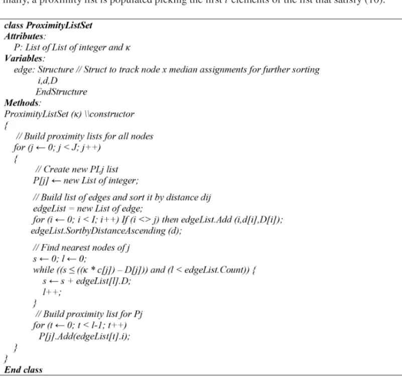
3.4 The Proximity List Set
The Proximity List Set(PL)is a data structure used to limit the number of iterations performed by aλ-interchange mechanism, during the intensification phase of CRO. Theλ-interchange mecha-nism is described in section 3.5.3. Due to the size of some of the instances that are evaluated in our tests, it becomes necessary to employ a strategy to reduce the number of interchange and shift operations that are typical of such algorithm. That is especially important on instances where p
is high. In a traditionalλ-interchange, every customer or group of customers is systematically relinked to all selected stations, other than the one they are currently assigned to, one station at a time, looking for possible improvements in the objective function value. In our version, we only consider for relinking, the selected stations that are in the vicinity of the station that a customer, or a group of customers, is currently assigned to. To accomplish that, for every node we build a static list containing nodes that are near that particular node. We call it a Proximity List. A Proximity List Set is a set of Proximity Lists of size J. Each element P L jcontains a list of stations that are near station j. The method used to populate the lists of nearby stations is an adaptation of an heuristic proposed by Stefanello et al. (2015), which was originally designed to eliminate decision variables that are unlikely to belong to good or optimal solutions.
Consider a decision variablexj. We define a subsetP Lj ⊆ Jof the nearest nodes ofj as:
P Lj =
t ∈ J
Dt ≤κcj −Dj
(10)
where a nodetis nearer to jthant′ifdj t <dj t′. Thus, for a candidate median j ∈ J, we include
the variablextin the nearby station list ift ∈ P Lj. The parameterκ is an expand capacity factor used to control the size of the proximity lists. Figure 2 shows a feasible solution for one of the instances (lin318 040) we test in this paper. The nodes that are part of the Proximity List of station 122 forκ = 5 are marked with a cross. The dashed line demarcates the boundaries of it, i.e., the farthest nodes from station 122. For the feasible solution shown in the figure, three stations would be considered, by theλ-interchange mechanism, for relinking the customers of station 122. A higher value forκwould include other nearby stations and vice-versa.
Fi
gur
e
2
–
Pr
oxi
m
it
y
Li
st
fo
r
st
a
ti
o
n
122
of
in
st
ance
li
n318
well as their demand(Di). Then, the resulting list of edges is sorted bydi j, in ascending order. Finally, a proximity list is populated picking the firsttelements of the list that satisfy (10).
Figure 3–The ProximityListSet class.
3.5 Elementary Reactions
constraint violation (7), the solution is rejected. Additionally, for a solution to be accepted, it must pass CRO’s own acceptance energy-based mechanisms, which are succinctly described in this paper. More information about CRO’s inner workings can be found in Lam & Li (2010, 2012).
3.5.1 On-wall ineffective collision
It happens when a molecule collides with the wall of a container and bounces back, remaining a single molecule. In this type of collision, the existing solutionωis perturbed to becomeω′, i.e.,
ω→ω′. This is done by generating aω′that is in a neighborhood ofω, through aλ-interchange operator, which was proposed by Osman & Christofides (1994).
LetN(·)be aλ-interchange neighborhood search operator. Therefore, we haveω′ = N(ω)and
P Eω′= f(ω′). In this type of reaction, typically, a potential energy loss will occur, i.e., P Eω′
will be less thanP Eω, indicating that a better solution has been obtained. If that does not occur and P Eω′ is greater than P Eω, then the worse solution can still be accepted, provided that
P Eω+K Eω ≥ P Eω′. However, every time a reaction occurs, a certain amount of kinetic energy(K E)is transferred to the energy buffer, decreasing the likelihood that worse solutions will be accepted on further iterations. The amount of kinetic energy of the molecule obtained from the ineffective reaction is controlled indirectly by the parameterKElossRate, which is a value between 0 and 1, inclusive, and affects the minimum amount of kinetic energy that is withdrawn from the original solution(ω).
3.5.2 Intermolecular ineffective collision
It occurs when two molecules collide with each other and then bounce away. The number of molecules remains unchanged, i.e.,ω1+ω2 → ω1′ +ω′2. This reaction is very similar to the on-wall ineffective collision, thus the sameλ-interchange operator from the on-wall ineffective collision is utilized. Let N(.)be aλ-interchange operator. Therefore, ω1′ andω′2are obtained throughω′1 = N(ω1)andω′2 = N(ω2). Energy management is similar to on-wall ineffective collisions, but does not involve the energybuffer.
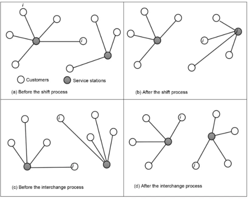
3.5.3 Theλ-interchange neighborhood search mechanism
For all on-wall and intermolecular ineffective collisions we implement a neighborhood search operator based on theλ-interchange mechanism, proposed by Osman & Christofides (1994) for the capacitated clustering problem (CCP). Theλ-interchange mechanismitself is an adaptation of a generation mechanism calledλ-opt procedure based on arcs-exchange, proposed by Lin (1965) for the Traveling Salesman Problem (TSP).
Theλ-interchange generates new neighborhoods as follows: LetCi be a cluster comprised of a number of customers assigned to a station (median),ζi. Given a solutionS = {C1, . . . ,Ci, . . . ,
andCj is a replacement of a subsetCi ⊆Ci of size|Ci| ≤λby another subsetCj ⊆Cj of size |Cj| ≤λto get two new clusters
Ci′ =(Ci −Ci)∪Cj and C′j =(Cj −Cj)∪Ci,
with possibly new different mediansζi′ andζ′j, respectively. The new solution becomes S′ = {C1, . . . ,C′i, . . . ,C′j, . . . ,Cp}. The neighborhoodN(S)ofSis the set of allS′solutions gener-ated by theλ-interchange mechanism for a given integerλand it is denoted byNλ(S).
Let P Li be a proximity list containing nodes nearζi (the median of clusterCi) andmi be the number of nodes in P Li which are also medians. Theλ-interchange mechanism will only ex-amine the pairs of clusters(Ci,Cj)whereζj ∈ P Li. Therefore, the number of different pairs of clusters(Ci,Cj)to be examined ismi, for a givenλ.
For any given pair of clusters(Ci,Cj), theλ-interchange mechanism utilizes two processes to generate neighborhoods. Let µ be the number of customers fromCi orCj to be handled by any of these two processes: a shift process tries to move µcustomers from clusterCi toCj, or vice-versa. Forµ = 1, a shift process is represented by the(0,1)and(1,0)operators. An interchange process, as the name implies, attempts to swap every customer from the first cluster with every other customer in the second cluster and, forµ=1, it is represented by the operator
(1,1).
Figure 4 illustrates the aforementionedshiftandinterchangeprocesses for a 1-interchange mech-anism(λ= 1). A shift process occurs from Figure 4(a) to Figure 4(b), where a customeri is shifted by the(1,0)operator. As a result, customer jbecomes the new median. Figure 4(c) and Figure 4(d), show the change in the clusters after customersiand jare interchanged, which also causes the medians to change on both clusters.
We implement a different order of search than the one employed by Osman & Christofides (1994). First, we attempt to swap customers before trying to shift them. This has proven to be more effective in our tests. Therefore, the order of operators becomes (1,1), (1,0) and (0,1). For the case ofλ = 2, the order of operations we used is (1,1), (1,0), (0,1), (1,2), (0,2), (2,1), (2,0), (2,2).
Our implementation ofλ-interchange mechanism is described as follows:
Upon start, a Proximity List Set is recomputed for an initialκ(κ0). Then, starting with a feasible solutionS, theλ-interchange logic is executed for a specific number of iterations, in an attempt to improve the current solution. In the end, the best solution is returned. The iterative process of theλ-interchange is shown below.
Figure 4–The 1-interchage mechanism(λ=1), adapted from Osman & Christofides (1994).
improvement in the objective function, one medianζifrom the incumbent solutionSis randomly interchanged with another nodeζj|ζj ∈/ S,ζj ∈ P Li. Both measures combined should allow new neighborhoods to be reached on subsequent iterations.
The process finishes when a specific number of iterations without improvement is reached. The number of iterations is proportional to the molecule’sNumHit, which is the total number of hits (collisions) that a molecule has suffered, so far. The actual number of iterations, for a given execution of theλ-interchange mechanism, is determined by multiplyingNumHitby a minimum number of iterations (Minλ-InterchangeIterations), which is typically a small integer, such as 1 or 2. This allows the first ineffective reactions to occur very fast, ruling out molecules that do not carry promising solutions. These molecules will quickly become targets for decompositions and syntheses, as they will not show improvements fast enough and will lose kinetic energy rapidly. On the other hand, molecules that carry better solutions tend to survive longer, as with every new collision they will be given a higher iteration limit.
According to Osman & Christofides (1994), a solutionSisλ-optimal (λ-opt) if, and only if, for any pair of clustersCi,Cj ∈S, there is no improvement that can be made by anyλ-interchange move. The authors also state that, in order to produce an efficient λ-opt descent algorithm it is advisable to produce a 1-opt solution. In our version of the λ-interchange mechanism, we follow this recommendation, by always obtaining a 1-opt solution before improving it to a 2-opt solution. Due to high computational costs of such mechanism, we limitedλto a maximum value of two. All on-wall collisions obtain a 1-opt solution, whereas intermolecular ineffective collision obtain a 2-opt solution, if necessary. The approximate rate of 1-opt to 2-opt solutions is 10, and it’s controlled by setting CRO’s parameter Molecollto 0.1. The pseudocode for the
λ-interchange mechanism is shown in Figure 5.
3.5.4 Decomposition
A decomposition occurs when a molecule(ω)collides with a wall and then breaks down in two pieces, producingω′1andω2′, that is:ω→ω′1+ω′2. The purpose of decomposition is to allow the system to explore other regions of the solution space, after having made considerable local search through ineffective collisions. Since more solutions are created, the total sum of P E
and K E of the original molecule may not be sufficient. In other words, we can have P Eω+
K Eω <P Eω′1+P Eω2′. Since energy conservation is not satisfied under these conditions, this decomposition must be aborted. To increase the chance of having a complete decomposition, a small portion of the energybufferis withdrawn to support the change.
We use the Half-total Change (HTC) operator to generate new solutions through decomposition. As the name implies, a new solution is produced from an existing one, keeping half of the existing values (medians) while assigning new values to the remaining half. Suppose we try to produce two new solutionsω′1= [ω′1(i),1≤i ≤ p]andω′2= [ω′2(i),1≤i ≤ p]fromω= [ω(i),1≤
For each of these elements, a new median is chosen at random, as long as it does not violate any of the problem constraints. Since elements are chosen randomly,ω1′ andω′2are very different from each other and also fromω′. In the present implementation, the half-total change operator ensures that the elements ofω′are present on eitherω′1orω′2, but not on both. Therefore, all medians fromω′will exist either onω′1orω′2.
The HTC operator takes as input a molecule’s Minimum Structure(MinStruct), which stores the best solution achieved by the molecule, and returns two output solutions,ω1′ andω2′. Initially, the process described above is repeated 100 times for each of the output solutions,ω′1andω′2. Then, we choose the bestω′1andω′2. Before the newly created solutions are returned to the main algorithm, both solutions are improved using the same process depicted on items 3.2b to 3.2e.
3.5.5 Synthesis
It is the opposite of decomposition. A synthesis occurs when two molecules collide and are fused together, that is: ω1+ω2 → ω′. In this reaction, a much larger change is allowed forω′ with respect toω1 andω2, along with a considerable increase in the kinetic energy of the resulting molecule. Therefore, it has a greater ability to explore its own solutions space, due to its higher kinetic energy.
We use a Distance Preserving Crossover (DPX) operator to carry out the synthesis of two molecules in a single molecule. The DPX operator was used by Merz & Freisleben (1997) to solve the quadratic assignment problem (QAP) through a Genetic Algorithm. It has proven to be well adapted to the CPMP problem. Letπ1andπ2be valid solutions for a given problem. The distanceT, between solutions, is defined as:
T(π1, π2)=
{i ∈ {1, . . . ,n}
π1(i)=π2(i)}
(11)
As defined in (11),T represents the number of selected stations present inπ1, which are not in
π2. The DPX operator aims to produce a descendant that has the same distance from each of its parents, being that distance equal to the distance between the parents themselves. Let A and B be two parents, with both A and B containing feasible solutions. First, all stations (medians) which are present on both parents are copied to descendant C. The remaining positions are then randomly populated with stations not yet assigned to any of its parents, ensuring that no station found in only one parent is copied to the descendant. This way, we obtain a descendant C, for which the conditionT(C,A)=T(C,B)=T(A,B)holds. Such crossover is highly disruptive, forcing subsequent local searches to explore different regions of the solution space, where better solutions could be found. If a feasible solution cannot be obtained, the synthesis fails.
The DPX operator takes as input the Minimum Structure(MinStruct)of two molecules,ω1and
it goes through an improvement process, which is the same as the one depicted on items 3.2b to 3.2e.
3.5.6 Energy conservation
In CRO, energy cannot be created or destroyed. The total energy of the system is determined by the objective function values, i.e., the P E of the initial molecules’ population, whose size is determined byPopSize, the initialK Eassigned to them and the initial energy value of thebuffer. In all experiments, we set thebuffer’s initial value to zero.
3.6 Initialization
Upon start, we set scalar variables corresponding to CRO standard operational parameters, which arePopSize,KELossRate,MoleColl,buffer,InitialKE,αandβ. In addition to CRO’s standard parameters, we set a few other parameters specific to our implementation, as follows:
• λ: it controls the highestλ-optsolution to be obtained by theλ-interchangemechanism. For example, ifλ=2, only 1-opt and 2-opt solutions will be computed by the mechanism.
• Minλ-InterchangeIterations: it is the starting number of iterations without improvement to be executed by aλ-interchange mechanism. The actual number of iterations for a given molecule isMinλ-InterchangeIterations * (NumHit + 1).
• MinMol: it is the minimum number of molecules in the population. If the population reaches this threshold, no syntheses will occur.
• MaxMol: it is the maximum number of molecules in the population. If the population reaches this threshold, no decompositions will occur.
• MaxIterations: it is the maximum number of iterations for the main CRO algorithm.
• MaxIterationsWithoutImprovement: it is the maximum number of iterations without im-provement in the objective function, for the main CRO algorithm.
• κ0: it is the initial value for the Proximity List Set capacity factor(κ). It is used in the
λ-interchange mechanism to indirectly influence the size of the lists in the Proximity List Set, as explained in sections 3.4 and 3.5.3.
• κ: capacity factor increment, used by the Proximity List Set in theλ-interchange mech-anism, as explained in section 3.5.3.
3.7 Iterations and finalization
During a single iteration, a molecule can collide with the wall of a container or with another molecule. This is decided by generating a random numberbbetween[0,1]. Ifb >MoleColl, a unimolecular collision occurs. Otherwise, an intermolecular collision takes place. In a uni-molecular collision, we randomly select a molecule from the population and decide if an on-wall inefficient collision or a decomposition occurs, according to a decomposition criterion, which is defined as: NumHit−MinHit> α(12). For an intermolecular collision, two molecules are randomly selected and then we determine if an intermolecular collision or a synthesis happens by checking the synthesis criteria for the chosen molecules, which is defined asK E=β(13). The inequalities (12) and (13) control the degree of diversification through a andβ parameters. Adequateαandβvalues allows a good balance between diversification and intensification. After an elementary reaction occurs, we check if the energy conservation condition is obeyed. If this has not happened, the change is discarded. Next, we check if the solution produced by the collision has a lower objective function value than the best solution we have obtained in the population, thus far. If so, we replace the best solution with the incumbent solution.
If none of the stopping criteria is reached, we begin a new iteration. Otherwise, we exit the main loop and return the best solution found. The number of iterations is controlled byMaxIterations
andMaxIterationsWithoutImprovement, as described in section 3.6. The main algorithm for the CRO is shown in Figure 6.
The pseudocodes for both ineffective reactions, synthesis and decomposition have not changed significantly from the tutorial, which the present implementation is based upon, and can be found on Lam & Li (2012).
4 COMPUTATIONAL RESULTS
4.1 Benchmark Datasets
The second dataset, proposed by Lorena & Senne (2004), is comprised of six instances, named sjc1 to sjc4b, built from data gathered from a geographic database of the city of S˜ao Jos´e dos Campos, Brazil. The number of nodes vary from 100 to 400 and the number of medians from 10 to 40. We compare the accuracy of our CRO for the CPMP with results available in the recent literature from Scheuerer & Wendolsky (2006) who developed a Scatter Search heuristic (SS) and with a Variable Neighborhood Search combined with CLEX from Fleszar & Hindi (2008). We also compare with a Clustering search heuristic from Chaves et al. (2007) and a Fenchel cutting planes allied with CPLEX approach (Fen-CPLEX) from Boccia et al. (2008). Addition-ally, the accuracy and computational time of our solution is compared with results obtained from solving the same problems using IBM CPLEX vs. 12.3 and the matheuristic IRMA, proposed by Stefanello et al. (2015), on similar hardware.
The last three datasets we utilize for accuracy and computational time comparisons, was pro-posed by Stefanello et al. (2015) and is originally comprised of 6 data sets of 5 instances each, adapted from TSP-LIB, with number of nodes varying from 318 to 4461 and number of medians varying from 5 to 1000. Since the present work is focused on instances of up to 724 nodes, we solve only the first three data sets. Larger instances will be tackled by a parallelized version of our CRO for the CPMP in a future article. However, most of the instances from the first three datasets cannot be solved to optimality by MIP solvers in a timely fashion, which justifies the use of heuristics.
All algorithms are coded in C# programming language and run on an Intel i7 2.3 GHz PC with 16 GB of RAM. After proper tune up, we solve all instances 20 times, recording execution times and objective function values. We also record the best objective and standard deviation. In addition to solving the instances using our CRO for the CPMP, the first dataset is solved by CPLEX vs.12.6, running on the same hardware.
4.2 Parameter tuning procedures
Our parameter tuning procedures are developed based on the premise that a good heuristic should provide acceptable results, that is, optimal or near optimal objective function values in rather short computational times. Therefore, during our tests we privilege low execution times over achieving optimality. Moreover, we try to achieve a gap of less than 1% on all tested instances. In the present work, we define gap as the percentage difference between the objective function values obtained by CRO, or any other metaheuristic or MIP solver, and the best-know value for a given instance.
sizes are controlled byMinMolandMaxMolparameters, respectively. Finally,κ0andκ con-trol the size of the Proximity List Set(P L)lists. Therefore, there is a total of 15 parameters that can affect CRO’s performance. Since the combination of parameters exist in a fifteen-dimension space, it is impractical to test all possible combinations. Instead, the parameters are tuned in an ad-hoc manner. Following is a brief discussion on the methodology we use for tuning and some empirical findings that may help in tuning similar CRO implementations.
We have empirically determined that the best results are achieved when the number of synthe-ses and decompositions is below 10% of the total number of collisions. This is in accordance with Lam & Li (2012), who state that “decomposition and synthesis bring diversification to the algorithm. Diversification cannot take place too often, or CRO will be become a completely random algorithm”. We have also empirically found that, for a givenKELossRate,MoleColland
InitialKE, the number of decompositions is highly dependent onα. If αis too low, e.g. less than two, molecules carrying solutions, may not have enough time (expressed in number of col-lisions) to achieve local minima. On the other hand, if a is too high, decompositions may never occur. Similarly, the number of syntheses is highly dependent onβ. If it is too close toInitialKE, syntheses will happen more often than desired, thus hurting intensification. Ifβ is too low, the number of synthesis collisions may not suffice.
Another important consideration when choosing appropriate values for the various CRO pa-rameters is population control. If the number of syntheses and decompositions is unbalanced, population will rapidly reachMinMolorMaxMol.
We choose anInitialKEthat is about the 10 to 20 times higher than the best-known objective for the problems we tested. WhenInitialKEis too low, most decompositions may be rejected, due to a lower tolerance to accept poorer solutions. Similarly, syntheses may start occurring too soon. Finding a suitable value forMoleCollis also very important. We choose 0.1 for all of our ex-periments, which means the probability of intermolecular collisions to happen is 0.1. Since the number of on-wall collisions is much higher, we always run a 1-opt (λ=1 or 1-interchange) op-timization for those. That has proven to be adequate for several instances to achieve optimality. For intermolecular collisions, we run a 1-opt optimization or a 2-opt optimization if we cannot achieve satisfactory results. Running a 2-interchange logic requires considerably more time, as the number of comparisons increase substantially. In addition, a 2-opt optimization is executed for each of the two molecules involved in the collision. Using a higherλis impracticable due to the dramatic increase in execution times.
Starting with typical values suggested in Lam & Li (2012), we empirically determine that the following parameters’ initial values work well with most of the tested instances:PopSize=10,
KELossRate=0.8,MoleColl=0.1,InitialKE=1,000,000,α =10,β =5,000, andbuffer
=0. After proper tuning, we set the additional parameters from our implementation of the CRO for the CPMP to: MinMol= 2,MaxMol=100,Minλ-InterchangeIterations=1,κ0 =1 and
To tune the parameters which provide stopping criteria (MaxIterationsand MaxIterationsWith-outImprovement) we solve a particular instance 20 times using our CRO for the CPMP, starting from a rather small value forMaxIterationsandMaxIterationsWithoutImprovement, such as 50 iterations. If an average gap, for the objective function, of less than 1% is obtained and at least one run achieves the best-know value for the objective function, we use that number of iterations asMaxIterationsWithoutImprovementand setMaxIterationsto be twice as many. Otherwise, we keep increasingMaxIterationsandMaxIterationsWithoutImprovementby a small amount, such as 50 iterations, until a gap of less than 1% with one optimal (or best-known) run is obtained or there is no significant improvement in the objective function. If those criteria cannot be fulfilled, we chose the run with the lowest gap. Additionally, we first try to solve an instance running a 1-interchange logic for all on-wall and intermolecular collisions. If the desired gap could not be obtained, then we use a 2-interchange logic for intermolecular collisions only. This is to avoid the performance penalty mentioned earlier. Once we find suitable values forMaxIterationsand
MaxIterationsWithoutImprovement, we solve the instance another 10-30 times, depending on the data set, and use the results in our comparison with other metaheuristics.
Many other tuning methodologies may be used to tune CRO parameters. The one we present is merely one that works for the instances we test. It generates good solutions over a large spectrum of problem parameters in our empirical tests. It may be possible to find a methodology that generates better solutions or works faster. Therefore, we do not claim that our methodology is “optimal” in any sense.
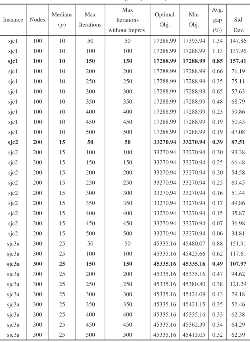
As an example of the tuning methodology we adopt, Figure 7 shows the objective function gap as a function ofMaxIterations, for the second benchmark dataset, proposed by Lorena & Senne (2004), which is comprised of six instances named sjc1, sjc2, sjc3, sjc3a, sjc4a and sjc4b. We use the same value forMaxIterationsandMaxIterationsWithoutImprovementon all execu-tions.MaxIterationsvaries from 50 to 500 iterations. The following CRO parameters are fixed:
PopSize=10,KeLossRate=0.8,MoleColl=1,InitialKe=1,000,000,A=10,B =5,000,
MinMol=2,MaxMol=20 andMinλ-InterchangeIterations=1. We run a 1-opt optimization (λ-interchange=1) on all instances, except for instance sjc4a, which we run a 2-opt optimization for all intermolecular collisions. For the same dataset, Table 2 shows the instance name, number of nodes, number of medians(p),MaxIterations,MaxIterationsWithoutImprovementand opti-mal value for the objective function as well as the lowest objective achieved by our CRO for the CPMP, the average percentage gap and the standard deviation for 20 runs of each combination of instance andMaxIterations(orMaxIterationsWithoutImprovement). Lines that meet the afore-mentioned criteria for tuningMaxIterationsandMaxIterationsWithoutImprovement(average gap of 1% or less with at least one run achieving the best-know value for the objective function, if possible) are marked in bold.
4.3 Results for Dataset 1
Table 2–Parameter tuning for sjc dataset (20 runs).
Instance Nodes Medians Max
Max
Optimal Min Avg.
Std
(p) Iterations Iterations Obj. Obj. gap
without Improv. (%) Dev.
sjc1 100 10 50 50 17288.99 17393.94 1.34 147.86
sjc1 100 10 100 100 17288.99 17288.99 1.13 137.96
sjc1 100 10 150 150 17288.99 17288.99 0.85 157.41
sjc1 100 10 200 200 17288.99 17288.99 0.66 76.19
sjc1 100 10 250 250 17288.99 17288.99 0.35 75.11
sjc1 100 10 300 300 17288.99 17288.99 0.65 57.63
sjc1 100 10 350 350 17288.99 17288.99 0.48 68.79
sjc1 100 10 400 400 17288.99 17288.99 0.23 59.86
sjc1 100 10 450 450 17288.99 17288.99 0.19 50.43
sjc1 100 10 500 500 17288.99 17288.99 0.19 47.08
sjc2 200 15 50 50 33270.94 33270.94 0.39 87.51
sjc2 200 15 100 100 33270.94 33270.94 0.30 93.38
sjc2 200 15 150 150 33270.94 33270.94 0.25 66.48
sjc2 200 15 200 200 33270.94 33270.94 0.20 54.58
sjc2 200 15 250 250 33270.94 33270.94 0.25 69.45
sjc2 200 15 300 300 33270.94 33270.94 0.16 51.44
sjc2 200 15 350 350 33270.94 33270.94 0.17 49.86
sjc2 200 15 400 400 33270.94 33270.94 0.15 35.87
sjc2 200 15 450 450 33270.94 33270.94 0.07 36.98
sjc2 200 15 500 500 33270.94 33270.94 0.06 34.81
sjc3a 300 25 50 50 45335.16 45480.07 0.88 151.91
sjc3a 300 25 100 100 45335.16 45423.66 0.62 117.61
sjc3a 300 25 150 150 45335.16 45335.16 0.49 107.97
sjc3a 300 25 200 200 45335.16 45335.16 0.47 94.62
sjc3a 300 25 250 250 45335.16 45380.80 0.38 121.29
sjc3a 300 25 300 300 45335.16 45424.09 0.43 79.18
sjc3a 300 25 350 350 45335.16 45421.15 0.35 52.46
sjc3a 300 25 400 400 45335.16 45335.16 0.33 62.38
sjc3a 300 25 450 450 45335.16 45362.39 0.34 64.29
Table 2–(Continuation).
Instance Nodes Medians Max
Max
Optimal Min Avg.
Std
(p) Iterations Iterations Obj. Obj. gap
without Improv. (%) Dev.
sjc3b 300 30 50 50 40635.90 40669.59 0.77 148.01
sjc3b 300 30 100 100 40635.90 40715.97 0.57 81.50
sjc3b 300 30 150 150 40635.90 40689.03 0.51 103.82
sjc3b 300 30 200 200 40635.90 40714.96 0.46 86.73
sjc3b 300 30 250 250 40635.90 40635.90 0.53 100.04
sjc3b 300 30 300 300 40635.90 40664.81 0.41 61.47
sjc3b 300 30 350 350 40635.90 40651.99 0.34 73.22
sjc3b 300 30 400 400 40635.90 40679.59 0.38 66.54
sjc3b 300 30 450 450 40635.90 40635.90 0.31 81.50
sjc3b 300 30 500 500 40635.90 40651.99 0.27 60.81
sjc4a 402 30 50 50 61925.51 62626.99 2.19 338.45
sjc4a 402 30 100 100 61925.51 62527.66 1.90 301.87
sjc4a 402 30 150 150 61925.51 62460.81 1.50 213.19
sjc4a 402 30 200 200 61925.51 62414.62 1.47 260.53
sjc4a 402 30 250 250 61925.51 62351.35 1.22 130.20
sjc4a 402 30 300 300 61925.51 62330.35 1.20 185.05
sjc4a 402 30 350 350 61925.51 62403.76 1.24 215.55
sjc4a 402 30 400 400 61925.51 62240.75 1.06 199.39
sjc4a 402 30 450 450 61925.51 62311.56 1.05 162.92
sjc4a 402 30 500 500 61925.51 62330.35 1.00 126.85
sjc4b 402 40 50 50 52458.00 52495.56 0.58 110.78
sjc4b 402 40 100 100 52458.00 52629.75 0.57 78.04
sjc4b 402 40 150 150 52458.00 52569.75 0.53 74.85
sjc4b 402 40 200 200 52458.00 52568.76 0.55 71.12
sjc4b 402 40 250 250 52458.00 52495.56 0.45 117.54
sjc4b 402 40 300 300 52458.00 52543.17 0.48 87.26
sjc4b 402 40 350 350 52458.00 52565.41 0.47 80.68
sjc4b 402 40 400 400 52458.00 52548.50 0.49 100.83
sjc4b 402 40 450 450 52458.00 52523.13 0.38 77.31
Figure 7–Objective function gap×MaxIterationsfor the sjc dataset.
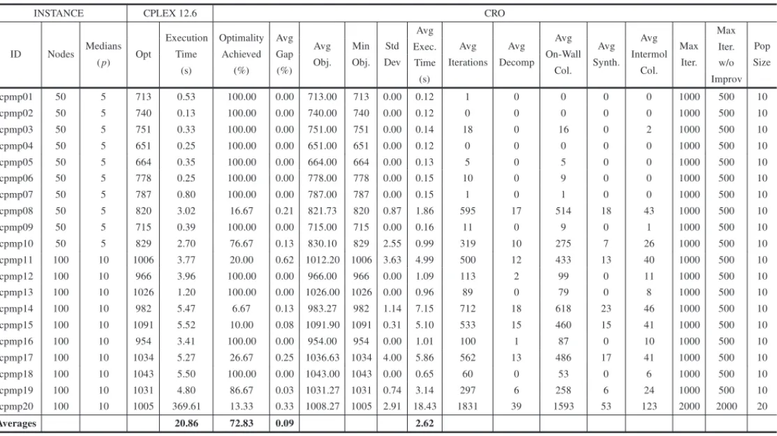
optimality by CPLEX. Table 3 shows the optimal objective function value (opt) and respective execution time to solve it using CPLEX. Then, we use CRO to solve each instance 30 times. The main algorithm stops whenMaxIterationsorMaxIterationsWithoutImprovementis reached. It also stops if, at any given iteration, the optimal value for the objective function is reached. For each test instance, we compute the percentage of times optimality was achieved, the average gap, the average and minimum objectives obtained, the standard deviation, the average execution time, the average number of decompositions, on-wall collisions, syntheses and intermolecular collisions. These results are also shown in Table 3, as well as the values we set for MaxItera-tions,MaxIterationsWithoutImprovementandPopSize. All other CRO parameters remain con-stant across all instances:KELossRate=0.8,MoleColl=0.1,InitialKE=1,000,000,α=10,
β =50,000,buffer=0,MinMol=2,MaxMol=100,Minλ-InterchangeIterations=1,κ0=1 andκ=1. A 1-opt optimization is used on all ineffective collisions.
In our experiments, CRO reaches the optimal value at least twice on all of the test instances; with the worst gap of 0.62% on instance cpmp11. The average of all gaps is of 0.089%. Notice that the constructive algorithm is able to generate an optimal solution for instances cpmp02 and cpmp04. Therefore, the average number of iterations is zero.
On average, CRO is 18.24s faster than CPLEX, with an average execution time of 2.62s versus 20.86s of CPLEX. CRO is slightly slower when solving instances 11, 14 and 17. However, the differences in execution time do not exceed 1.7s.
DA N IL O C ´ESAR AZ ER ED O SI LV A a n d M ´AR IO M EST R IA
Table 3–Computational results of CRO for dataset 1 (30 runs).
INSTANCE CPLEX 12.6 CRO
ID Nodes Medians Opt
Execution Optimality Avg
Avg Min Std Avg
Avg Avg Avg Avg Avg Max
Max Pop
(p) Time Achieved Gap Obj. Obj. Dev Exec.
Iterations Decomp On-Wall Synth. Intermol Iter. Iter.
Size
(s) (%) (%) Time Col. Col. w/o
(s) Improv
cpmp01 50 5 713 0.53 100.00 0.00 713.00 713 0.00 0.12 1 0 0 0 0 1000 500 10
cpmp02 50 5 740 0.13 100.00 0.00 740.00 740 0.00 0.12 0 0 0 0 0 1000 500 10
cpmp03 50 5 751 0.33 100.00 0.00 751.00 751 0.00 0.14 18 0 16 0 2 1000 500 10
cpmp04 50 5 651 0.25 100.00 0.00 651.00 651 0.00 0.12 0 0 0 0 0 1000 500 10
cpmp05 50 5 664 0.35 100.00 0.00 664.00 664 0.00 0.13 5 0 5 0 0 1000 500 10
cpmp06 50 5 778 0.25 100.00 0.00 778.00 778 0.00 0.15 10 0 9 0 0 1000 500 10
cpmp07 50 5 787 0.80 100.00 0.00 787.00 787 0.00 0.15 1 0 1 0 0 1000 500 10
cpmp08 50 5 820 3.02 16.67 0.21 821.73 820 0.87 1.86 595 17 514 18 43 1000 500 10
cpmp09 50 5 715 0.39 100.00 0.00 715.00 715 0.00 0.16 11 0 9 0 1 1000 500 10
cpmp10 50 5 829 2.70 76.67 0.13 830.10 829 2.55 0.99 319 10 275 7 26 1000 500 10
cpmp11 100 10 1006 3.77 20.00 0.62 1012.20 1006 3.63 4.99 500 12 433 13 40 1000 500 10
cpmp12 100 10 966 3.96 100.00 0.00 966.00 966 0.00 1.09 113 2 99 0 11 1000 500 10
cpmp13 100 10 1026 1.20 100.00 0.00 1026.00 1026 0.00 0.96 89 0 79 0 8 1000 500 10
cpmp14 100 10 982 5.47 6.67 0.13 983.27 982 1.14 7.15 712 18 618 23 46 1000 500 10
cpmp15 100 10 1091 5.52 10.00 0.08 1091.90 1091 0.31 5.10 533 15 460 15 41 1000 500 10
cpmp16 100 10 954 3.41 100.00 0.00 954.00 954 0.00 1.01 100 1 87 0 10 1000 500 10
cpmp17 100 10 1034 5.27 26.67 0.25 1036.63 1034 4.00 5.86 562 13 486 17 41 1000 500 10
cpmp18 100 10 1043 5.50 100.00 0.00 1043.00 1043 0.00 0.65 60 0 53 0 6 1000 500 10
cpmp19 100 10 1031 4.80 86.67 0.03 1031.27 1031 0.74 3.14 297 6 258 6 24 1000 500 10
cpmp20 100 10 1005 369.61 13.33 0.33 1008.27 1005 2.91 18.43 1831 39 1593 53 123 2000 2000 20
Averages 20.86 72.83 0.09 2.62
Table 4–Comparison of CRO with other heuristics for dataset 1.
Instance CRO IRMA(α=2.4) SATS SA TS
ID Opt. Best gap Exec. Time Best gap. Exec. Time Best gap Best gap Best gap
(%) (s) (%) (s) (%) (%) (%)
cpmp01 713 0.00 0.11 0.00 0.20 0.00 2.94 2.94
cpmp02 740 0.00 0.11 0.00 0.05 0.00 0.00 0.00
cpmp03 751 0.00 0.12 0.00 0.16 0.00 0.00 0.00
cpmp04 651 0.00 0.11 0.00 0.08 0.00 0.00 0.00
cpmp05 664 0.00 0.12 0.00 0.15 0.00 0.00 0.00
cpmp06 778 0.00 0.12 0.00 0.08 0.00 0.00 0.00
cpmp07 787 0.00 0.12 0.00 0.35 0.00 2.28 0.00
cpmp08 820 0.00 0.86 0.00 4.65 0.00 0.00 0.12
cpmp09 715 0.00 0.12 0.00 0.24 0.00 0.00 0.00
cpmp10 829 0.00 0.13 0.00 0.89 0.00 0.00 0.00
cpmp11 1006 0.00 0.63 0.00 1.83 0.00 0.00 0.29
cpmp12 966 0.00 0.2 0.00 1.23 0.00 0.00 0.20
cpmp13 1026 0.00 0.24 0.00 0.43 0.00 0.00 0.00
cpmp14 982 0.00 1.8 0.00 5.15 0.30 0.00 0.30
cpmp15 1091 0.00 3.09 0.00 6.57 0.00 0.00 0.36
cpmp16 954 0.00 0.23 0.00 0.80 0.00 0.00 0.31
cpmp17 1034 0.00 0.32 0.00 2.16 0.48 0.29 0.58
cpmp18 1043 0.00 0.22 0.00 2.26 0.19 0.19 0.19
cpmp19 1031 0.00 0.32 0.00 2.42 0.00 0.09 0.29
cpmp20 1005 0.00 4.61 0.00 64.49 0.00 1.39 0.00
Averages 0.00 0.68 0.00 4.71 0.05 0.36 0.28
Finally, we compare our results with the matheuristic IRMA, proposed by Stefanello et al. (2015), which combines local search based metaheuristics and mathematical programming techniques to solve the capacitatedp-median problem. To provide a fair comparison between CRO and IRMA, from the various IRMA test results available for Dataset 1 we choose the one that achieved optimality on all test instances (IRMAα =2.4), this making it at par with our implementation of the CRO, in terms of accuracy. Since IRMA was tested on modern hardware (Intel i5-2300 2.8 GHz CPU PC with 4 GB RAM) a fairer comparison of execution times can be done: CRO is faster IRMA on half of the tested instances, as shown in Table 4. However, the average execution time of IRMA is 4.71s versus 2.62s of CRO, thus making it slightly faster.
4.4 Results for Dataset 2
The second dataset we use to evaluate our CRO for CPMP is comprised of 6 instances proposed by Lorena & Senne (2004). We solve all problems 30 times using CRO and compare the accuracy and execution times of our results with the ones obtained Stefanello et al. (2015), using the matheuristic IRMA, which combines a model reduction heuristic and a MIP solver (CPLEX 12.3). In their work, Stefanello solved the full model for all sjc problems using IBM CPLEX. We use these results in our comparisons as well, since their hardware platform and CPLEX version are very similar to ours. In addition, we compare the accuracy of our CRO with results available in the recent literature from Scheuerer & Wendolsky (2006), who developed a Scatter Search heuristic (SS), a Variable Neighborhood Search (VNS) combined with CLEX from Fleszar & Hindi (2008), a Clustering search heuristic (CS), from Chaves et al. (2007) and a Fenchel cutting planes and CPLEX based approach (Fen-CPLEX) from Boccia et al. (2008). It is important to notice that, in spite of being relatively recent works, the hardware platforms utilized by these authors can be considered obsolete, consisting of a low-end Intel Celeron 2.2 GHz, an Intel Pentium IV 3.2 GHz, an Intel Pentium IV 3.02 GHz and an l.6 GHz processor running on a laptop computer, respectively. Therefore, we provide a speed comparison for reference purposes only, as it would not be fair to compare CRO results with the ones published by the aforementioned authors, considering that these processors were released more than a decade ago. Another reason is that the execution times reported by the authors are, on average, 28 to 197 times slower than the times reported by Stefanello et al. (2015), thus making a speed comparison less relevant. The same stopping criteria and computations from dataset 1 are employed on dataset 2. The other CRO parameters that remain constant across all instances are: KELossRate= 0.8, MoleColl
C H EM IC AL R EA C T IO N O PT IM IZ A T IO N M ET AH EU R IST IC F O R L O C A T IN G SER VI C E ST A T IO N S
Table 5–Computational results of CRO for dataset 2 (30 runs).
INSTANCE CRO
ID Nodes Medians Opt
Optimality Avg
Avg Min Std
Avg
Avg Avg Avg Avg Avg Max
Max
Pop
α β
(p) Achieved Gap Obj. Obj. Dev
Exec.
Iterations Decomp On-Wall Synth. Intermol Iter. Iter.
Size
(%) (%) Time Col. Col. w/o
(s) Improv
sjc1 100 10 17288.99 36.67 0.49 17373.46 17288.99 72.23 3.08 221 3 193 0 23 300 150 10 10 50000
sjc2 200 15 33270.94 26.67 0.32 33377.71 33270.94 89.16 1.83 55 0 48 0 6 100 50 10 10 50000
sjc3a 300 25 45335.16 3.33 0.27 45457.79 45335.16 50.44 250.95 4136 473 3212 300 150 5000 2500 50 2 500000
sjc3b 300 30 40635.90 3.33 0.26 40740.45 40635.90 49.08 49.89 791 94 611 62 23 1000 500 10 2 500000
sjc4a 402 30 61925.51 0.00 0.82 62434.54 62157.19 84.78 211.64 854 15 748 9 80 1000 500 10 10 50000
sjc4b 402 40 52458.00 0.00 0.76 52854.97 52651.53 99.18 11.60 66 0 58 0 7 100 50 10 10 50000
Averages 0.49 88.17
DA
N
IL
O
C
´ESAR
AZ
ER
ED
O
SI
LV
A
a
n
d
M
´AR
IO
M
EST
R
IA
Table 6–Comparison of CRO with other heuristics for dataset 1.
Instance CRO CPLEX IRMA(α=2.4) SS VNS CS Fen-Cplex
ID Opt. Best gap Exec. Time Best gap. Exec. Time Best gap Exec. Time Best gap Exec. Time Best gap Exec. Time Best gap. Exec. Time Best gap Exec. Time
(%) (s) (%) (s) (%) (s) (%) (s) (%) (s) (%) (s) (%) (s)
sjc1 17288.99 0.000 1.17 0.000 4.89 0.000 1.90 0.000 60.00 0.000 50.50 0.000 22.72 0.000 37.60 sjc2 33270.94 0.000 0.53 0.000 11.46 0.000 3.25 0.068 600.00 0.000 44.08 0.000 112.81 0.000 127.90
sjc3a 45335.16 0.000 198.93 0.000 62.20 0.000 23.96 0.006 2307.00 0.000 8580.30 0.000 940.75 0.000 495.10
sjc3b 40635.90 0.000 1.30 0.000 16.14 0.000 2.47 0.000 2308.00 0.000 2292.86 0.000 1887.97 0.000 72.20 sjc4a 61925.51 0.374 116.79 0.000 215.60 0.000 56.67 0.000 6109.00 0.000 4221.47 0.005 2885.11 0.000 1209.50
sjc4b 52458.00 0.369 7.08 0.000 35.90 0.000 6.26 0.140 6106.00 0.023 3471.44 0.140 7626.33 0.000 669.70
Averages 0.124 54.30 0.000 57.70 0.000 15.75 0.036 2915.00 0.004 3110.11 0.024 2245.95 0.000 435.33
a
O
per
ac
ional,
V
ol.
38(
3)
,
C H EM IC AL R EA C T IO N O PT IM IZ A T IO N M ET AH EU R IST IC F O R L O C A T IN G SER VI C E ST A T IO N S
Table 7–Comparison of CRO with other heuristics for dataset 1.
Instance IRMA IRMA CRO
Phase 2 Phase 3
ID Nodes Med. BKS
Avg Avg Avg Avg Avg Avg
Runs BKS Avg Min Std Avg Avg
Avg
Avg
Avg Max
(p) Gap
Exec.
Gap Exec. Gap Exec.
Obj. Obj. Dev Iter. Dec.
On- Inter- Max Iter.
(%) Time (%) Time (%) Time (%) Wall Syn mol. Iter. w/o
(s) (s) (s) Col. Col. Impr
lin318 005 318 5 180281.21 0.00 9.15 – – 0.00 9.76 10 60.00 180281.67 180281.21 0.58 135 3 117 0 14 200 100
lin318 015 318 15 88901.56 0.00 26.35 – – 0.08 23.88 10 60.00 88972.76 88901.56 107.09 268 5 234 2 26 300 150
lin318 040 318 40 47988.38 1.01 222.41 0.14 319.46 0.65 97.76 10 0.00 48302.49 48175.96 143.22 483 4 424 8 44 500 250
lin318 070 318 70 32198.64 0.01 127.45 – – 1.02 728.49 10 0.00 32528.45 32333.03 110.87 3477 35 3063 42 189 4000 2000
lin318 100 318 100 22942.69 2.23 222.65 0.00 364.87 0.97 2075.61 10 0.00 23165.59 23058.23 54.68 3518 28 3109 35 167 4000 2000
ali535 005 535 5 9956.77 0.00 7.08 0.00 45.42 0.00 2.17 10 100.00 9956.77 9956.77 0.00 0 0 0 0 0 4000 2000
ali535 025 535 25 3695.15 0.24 311.36 0.00 544.26 0.07 348.36 10 0.00 3697.90 3696.56 1.18 883 12 777 19 47 1000 500
ali535 050 535 50 2461.41 1.69 377.28 0.00 726.30 1.58 842.99 10 0.00 2500.24 2480.37 14.50 983 7 867 14 55 1000 500
ali535 100 535 100 1438.42 2.61 362.75 0.02 637.64 3.17 1341.98 10 0.00 1483.98 1468.28 11.08 969 4 863 12 43 1000 500
ali535 150 535 150 1032.28 2.54 366.54 0.00 761.31 3.56 3621.14 10 0.00 1069.06 1057.06 9.78 953 3 845 11 47 1000 500
u724 010 724 10 181782.96 0.00 6.64 0.00 59.65 0.03 354.99 10 30.00 181842.37 181777.72 88.99 381 7 330 4 38 500 250
u724 030 724 30 95034.01 0.01 158.05 0.00 300.72 0.14 152.50 10 0.00 95168.34 95106.33 49.40 408 9 354 7 37 500 250
u724 075 724 75 54735.05 0.08 507.56 0.00 546.39 0.96 439.98 10 0.00 55261.34 55074.78 99.18 486 3 434 9 36 500 250
u724 125 724 125 38976.76 0.28 509.01 0.02 643.31 2.52 761.39 10 0 39957.9 39686.84 185.7 981 4 871 12 57 1000 500
u724 200 724 200 28079.97 0.10 508.81 0.11 706.29 2.75 2710.03 10 0 28853.36 28690.35 140.68 976 3 861 11 57 1000 500
Averages 0.72 248.21 0.02 471.30 1.17 900.74
but much faster than the other methods in the group. On average, it is 381.03s faster than Fen-Cplex, the third fastest method, and 3055.81s faster than VNS, the slowest one. Regarding optimality, SS achieved it in only 3 instances, being the worst in the group, whereas the other methods achieved optimality in 4 or more instances, thus matching or surpassing CRO. While the average of the best gaps achieved by CRO can be considered very satisfactory, in our opinion, it is higher than the other methods, especially the ones that used an MIP solver.
Despite not being the fastest or most accurate method in this comparison, we believe that our im-plementation of the CRO for CPMP may have a competitive advantage on applications that must run on less capable hardware. The reason is that it requires a much smaller memory footprint (typically less than 64 MB) and runs on a single CPU/Core, whereas most hybrid solutions that employ MIP solvers, such as IBM CPLEX, require large amounts of memory (typically more than 2GB) and multicore CPUs to perform well. The high cost of licensing an MIP solver may also be a limiting factor to such hybrid solutions. Furthermore, the average gap/processing time that can be obtained with CRO may be acceptable in many scenarios.
4.5 Results for Datasets 3, 4 and 5
The last three datasets we utilize for accuracy and speed comparisons was proposed by Stefanello et al. (2015) and is comprised of 3 data sets of 5 instances each, adapted from TSP-LIB, with 318 to 724 nodes and 5 to 200 medians. We solve all problems 10 times using CRO and compare the accuracy and execution times of our results with the ones obtained Stefanello et al. (2015), who also solved those 10 times using the matheuristic IRMA, which combines a model reduction heuristic and a MIP solver (CPLEX 12.3). We compare the average gaps and average execution times obtained by CRO with the ones obtained by Phase 2 and 3 of IRMA. Since most of these problems cannot be solved to optimality by MIP solvers in a timely fashion, we report in Table 7, their objective function values for the Best Know feasible Solution (BKS), regardless of being achieved by CRO or IRMA. Whenever optimal values are available, they are marked in bold. Table 7 shows the average gaps and average execution times for IRMA’s Phase 2 and Phase3, as well as for CRO. It also shows, for CRO only, the percentage of times BKS is achieved, the average and minimum objectives attained, the standard deviation, the average execution time, the average number of decompositions, on-wall collisions, syntheses and intermolecular collisions. At last, we report in Table 7 the values we set forMaxIterations, MaxIterationsWithoutImprove-mentandPopSize. All other CRO parameters remain constant across all instances: PopSize= 10;KELossRate=0.8,MoleColl=0.1,InitialKE=1,000,000,α= 10,β =100,000, buffer = 0,MinMol=2, MaxMol= 100 andMinλ-InterchangeIterations= 1. We setκ0 =1 and
κ =1 on all instances, but u724 125 and u724 200, which have bothκ0 andκ =1 set to 0.1. A 1-opt optimization is used on all ineffective collisions.
Test run results show that our CRO for the CPMP performs better when solving instances where