Earnings management around mergers and acquisitions

Martim Rúben Candeias Couto Pinto

Earnings Management Around

Mergers and Acquisitions

Mar

tim R

úben Candeias Cout

o Pint o Abril de 2016 UMinho | 20 16 Ear nings Manag ement Around Mer g er s and Acq uisitions

Universidade do Minho

Abril de 2016

Tese de Mestrado em Finanças

Trabalho efectuado sob a orientação do

Professor Doutor Gilberto Ramos Loureiro

Martim Rúben Candeias Couto Pinto

Earnings Management Around

Mergers and Acquisitions

Universidade do Minho

Escola de Economia e Gestão

Universidade do Minho

ii

DECLARAÇÃO

Nome: Martim Rúben Candeias Couto Pinto

Endereço eletrónico: martimonfire@gmail.com

Telefone: +351 914 010 531

Título dissertação: Earnings Management Around Mergers and Acquisitions

Orientador: Professor Doutor Gilberto Loureiro

Ano de conclusão: 2016

Designação do Mestrado: Mestrado em Finanças

É AUTORIZADA A REPRODUÇÃO INTEGRAL DESTA TESE/TRABALHO APENAS PARA EFEITOS DE INVESTIGAÇÃO, MEDIANTE DECLARAÇÃO ESCRITA DO INTERESSADO, QUE A TAL SE COMPROMETE;

Universidade do Minho, Abril de 2016

iii

ACKNOWLEDGEMENTS

This master dissertation could not be written to its fullest without Professor Dr. Gilberto Loureiro, who made himself available, and accepted to be my supervisor. He has never accepted anything less than my best efforts, and for that, I would like to express my deep gratitude. His professional nature, precise and methodical were vital in my development as a student. I have learned many things since I became Professor Dr. Gilberto Ramos Loureiro's student. He kept me going when times were tough, always asking insightful questions and offering invaluable advice. I have been lucky to have a supervisor who cared so much about my work, and who replied to my questions so promptly. My Erasmus period did not allow me to learn how to gather data and use the proper software for my master dissertation. Thus, my supervisor had extra work to provide me with the essential knowledge to use the necessary tools to develop my work. For everything you have done for me, Dr. Gilberto, I thank you.

Special thanks are given to Ricardo Pinto, my brother, for his continued support and encouragement throughout my studies and life, despite living in Canada. I am so lucky to have him as my brother. His love and moral support sustained me throughout. I was continually amazed by his willingness to proofread countless pages of meaningless text for him. The numerous hours that we passed on skype were incredibly helpful to me. Also my brother in law, Michael McManus, for such patience helping my brother reading my master dissertation.

I am grateful to Professor Dr. Florinda Silva and Professor Dr. Nelson Areal for their insightful comments and suggestions, and the others participants in the 4th edition of EEG Research Day (March - 2016) in the University of Minho, who contributed through important questions and valuable comments which increased the quality of my dissertation.

To the Minho University and Economy and Business School’s Teachers, specifically the ones from Masters in Finance for all their support.

A special thanks to my father, Arlindo Pinto, not only for his encouragement, faith in me, and financial support, but also, for allowing me to be as ambitious as I wanted, and pushed me to do more and better every day. He is the kind of father that is everything in our life, forgetting luxuries to be able to give me what he could not have.

iv I owe more than thanks to my other family members, which include my mother, Leonor Couto, my brother Miguel Pinto, my nephews, Daniel and Diogo, and all my uncles. My sister and brother in law, Liliana Marques and Nelson Marques, for their love and endless moral support.

I want also express my gratitude to Marta Silva, for her continued support, encouragement, patience, and unwavering love. My gratitude also goes to Mr. Silva and Mrs. Silva.

Last but not least, a big thanks also goes to friends made in the University and friends of long run, who provided a much needed form of escape from my studies, making me laugh often. This thanks belong especially to (without any order) Diamantina Marques, André Abreu, Diana Silva, Ricardo Barbosa, Raquel Silva, Zélia Fonseca, Ricardo Matos, Ricardo Filipe, João Silva, Ricardo Marques, Susana Freitas, Daniela Fernandes, Hélder Gonçalves, Cátia Costeira, Gabriela Coelho, Joana Silva and Alda Canito.

v

Earnings Management Around Mergers and Acquisitions

ABSTRACT

I examine whether acquirers use earnings management to boost their stock prices prior to announcing an acquisition where stock is used as a method of payment and the consequences of such activities in terms of post-operating performance. Consistent with previous studies, I document that managers of acquiring companies engage in more aggressive earnings management in cases of stock-financed acquisitions. Moreover, in cash-financed acquisitions there is no evidence at all of earnings management prior to the announcement of the deal. To measure the long-term performance, I use two methods – the operating income scaled by sales, and the buy-and-hold abnormal returns (BHAR). Previous studies have shown ambiguous evidence about the post-operating performance. In this study, using operating income scaled by sales, I report a statistically significant decrease in the post-operating performance. Also, using BHAR, I find that acquirers involved in stock-financed acquisitions exhibit poor log-term performance after the acquisition. In contrast, I find that in cash-financed deals, acquirers tend to perform better post-acquisition. In this dissertation, I contribute to the existing literature by examining the earnings management and post-acquisition performance of European Union firms involved in mergers and acquisitions (M&A).

Keywords: Earnings Management, Discretionary Accruals, Post-Acquisition Performance, Mergers and Acquisitions

vi

Manipulação de resultados entre fusões e aquisições

RESUMO

Neste estudo pretende-se detetar se nas fusões e aquisições as empresas compradoras recorrem à prática da gestão de resultados com o intuito de inflacionar os preços das suas ações, principalmente nos casos em que é realizada a compra através de ações. Além disso, também é analisado se a performance pós-aquisição é menor nestes casos. Os resultados indicam que a manipulação dos resultados das empresas, anterior à aquisição, é evidente nos casos em que o pagamento é feito por ações. Além disso, verifica-se que nas aquisições pagas em dinheiro não há nenhuma evidência de manipulação de resultados no ano anterior ao anúncio. Em relação ao desempenho pós-aquisição, são adotadas duas medidas – o resultado operacional dividido pelas vendas e o buy-and-hold abnormal returns (BHAR). Relativamente à performance operacional pós-aquisição, os estudos anteriores não são unanimes. Neste estudo são encontrados desempenhos pós-aquisições anormais estatisticamente significativos, usando a metodologia do lucro operacional dividido pelas vendas. Além disso, há evidência de que a performance de médio-longo prazo após a aquisição, medida pelos BHAR, é mais fraca para as empresas compradoras que pagaram as aquisições com ações. Isto é, após uma aquisição financiada por de ações do comprador, é experienciada uma rendibilidade anormal negativa num período até 3 anos. Contrariamente, nas aquisições financiadas em dinheiro há evidência de uma performance positiva (até 3 anos) após a aquisição. Esta dissertação contribui para a literatura existente ao analisar a existência de manipulação de resultados, e as suas consequências em termos de performance, nas empresas da União Europeia que se envolveram em fusões e aquisições. Palavras-chave: Manipulação de Resultados, Discretionary Accruals, Desempenho Pós-aquisição, Fusões e Aquisições.

vii

Index

2. Literature Review and Hypotheses Development ... 5

Earnings Management ...5

Discretionary Accruals and Non-Discretionary Accruals ...6

Motivations and Consequences of Earnings Management ...7

Earnings Management on Mergers and Acquisitions ... 10

Post-Acquisition Performance on Mergers and Acquisitions ... 11

Post-Acquisition Operating Performance ... 12

Buy and Hold Abnormal Return ... 13

Hypotheses to test ... 14

3. Data and Methodology ... 15

Data and Sample ... 15

Methodology ... 19

Calculation of the Earnings Management ... 19

3.2.1.1. Discretionary Total Accruals ... 19

3.2.1.2. Probit Multivariate Analysis ... 20

Calculation of the Long-Term Post-Acquisition Performance ... 22

viii

3.2.2.2. Buy-and-Hold Abnormal Returns Post-Acquisition ... 23

Descriptive statistics ... 25

4. Results ... 28

Earnings Management ... 28

Total Discretionary Accruals – Univariate Analysis ... 28

Probit Multivariate Analysis ... 29

Long-Term Post-Acquisition Performance ... 32

Post-Acquisition Operating Performance ... 32

Buy-and-Hold Abnormal Returns Post-Acquisition ... 35

5. Conclusions ... 46

6. References ... 48

ix

Table Index

Table 1 - Data Distribution ... 17

Table 2 - Descriptive Statistics – Method of Payment: Stock, Cash and Mixed ... 26

Table 3 - Total Discretionary Accruals - Univariate analysis... 29

Table 4 - Results from probit regressions of M&A ... 31

Table 5 - Op. income scaled by sales: Δ from t-1 to t+1, t+2 and t+3 (100% stock & 100% cash) ... 34

Table 6 - BHAR – 100% stock-financed & 100% cash-financed from t to t+1 ... 36

Table 7 - BHAR – Earnings management impact from t to t+1 t+2 t+3 ... 39

Table 8 - BHAR – EMt-1 / No EMt-1 with stock / with cash: from t to t+1, t+2 and t+3 ... 41

Table 9 - BHAR – EMt-1 Top / Low quartile - 100% stock / 100% cash: from t to t+1 ... 44

Figures Index

1

1. Introduction

After over 30 years of research in earnings management, the truth is that this is a common practice that still occurs nowadays. Managers may have incentives to manipulate their companies’ earnings to artificially boost the stock prices around some corporate events that yield superior outcomes when the firms’ equity is overvalued. However, this practice is not sustainable in the long-run and, eventually, in the aftermath of the event the stock price should revert to its normal value. In this dissertation, I study whether managers engage in more aggressive accrual-based earnings management prior to a stock-financed acquisition, as well as its consequences in terms of long-term post-operating and return performance.

By definition, a company’s main purpose is to maximize the value its stocks and therefore the wealth of their owners. If the market could fully observe the practice of earnings management and anticipate its negative impact on future long-term performance, managers would have no incentives to engage in such activities. However, due to information asymmetries between firm insiders and outsiders, managers have some latitude to engage in earnings management without being noticed. The pressure to deliver some short-term positive outcomes, gives managers an incentive to manipulate earnings upwards to boost the firm’s stock price.

Mergers and acquisitions (M&A) are faster ways of company expansion than internal, organic growth (Gaughan, 2007). It is perceived as a growth engine. Merger is a combination of two or more companies, usually a mutual decision among those firms. Accordingly to Vazirani (2015, p.3), a merger is “… a circumstance in which the assets and liabilities of a company (merging company) are vested in another company (merged company) [...], the shareholders of the merging company become shareholders of the merged company”. Acquisition, accordingly to Vazirani (2015, p.4) is “… a corporate action in which a company (acquirer) buys most, if not all, of the target company’s ownership stakes in order to assume control of the target firm […] it may be friendly0F

1 or hostile

1F

2 depending on a company’s willingness to be acquired”.

M&A historically around the world has been divided into merger waves. These waves usually start with intense merger activity followed by a period of slower merger activity. The six M&A waves recognized in the literature (Kummer & Steger, 2008) are the following (illustrated in Figure 1):

1 When the Board of Directors agrees with the acquisition.

2  First Wave 1897 – 1907: Horizontal Mergers

 Second Wave 1919 – 1933: Increasing Concentration  Third Wave 1955 – 1975: The Conglomerate Era

 Fourth Wave 1980 – 1989: The Retrenchment Era and Hostile takeovers  Fifth Wave 1992 – 2002: The Age of the Strategic Mega-Merger

 Sixth Wave 2003 – 2007: The Rebirth of Leverage

Figure 1 - Mergers and Acquisition Activity in The United States (1887 - 2007) - Adapted from “Why merger and acquisition (M&A) waves reoccur: The vicious circle from pressure to failure” by C. Kummer and U. Steger (2008), Strategic Management Review, 2(1), p. 44.2F

3

Vazirani (2015) and Alexandridis, Mavis and Travlos (2011) also recognize these six waves, although, with slight differences to the years mentioned by Kummer and Steger (2008).

The last wave ended when the subprime crisis arose (Aalbers, 2009). Each one had higher volume than the previous ones and were much more geographically dispersed (Kim & Zheng, 2014; Kummer & Steger, 2008).

Not disregarding the previous waves, the last one also affected Europe. Since my study is based in European Union countries from 2000 forward, the last M&A wave is fully included in my study. As

3 Aalbers (2009) states, “The crisis does not just hit investment banks on Wall Street, European banks and pension funds […], also individual investors and small towns around the globe”. M&A are typically paid in cash, stock, or a combination of these two. In acquisitions that involve stock as a method of payment, the acquirer can extract larger benefits from the deal when its stocks are overvalued. For instance, when a stock-financed deal is completed, the acquiring company gives a specific number of shares for each share of the target company. Initially, the acquiring and target firms agree on a specific purchase price. The number of shares from the acquiring firm exchanged for each share of the target firm is determined by the price of the acquiring firm’s stock when the merger agreement is reached, given the agreement upon the target firm purchase price. As a result, the higher the price of the acquiring firm's stock on the agreement date, the fewer the number of shares that must be issued to purchase the target firm (Erickson & Wang, 1999).Therefore, managers of acquiring firms may have a strong incentive to inflate earnings, and therefore, artificially increase the market value of their stocks prior to the acquisition. When firms inflate financial statements by managing their earnings, they could be expecting it to be reverted in the long-run after the deal is completed (L. J. Cohen, Cornett, Marcus, & Tehranian, 2014; Dechow, Sloan, & Sweeney, 1996; Paul Healy, 1985).

Pungaliya and Vijh (2009, p.2) state an interesting idea, “If academic researchers can detect earnings management in broad samples, then it is not entirely clear why target managers and investment bankers with greater access to firm-specific and industry-specific information cannot do the same”. This is probably explained by cash bonuses (side payments), golden parachutes or board membership position given to the target’s managers in the event of an acquisition (Hartzell, Ofek, & David, 2004).

Using a sample of 28 EU countries (where 2,763 acquirers made 5,982 acquisitions), over the period January of 2000 until December of 2014, I analyze if the likelihood of a stock-financed acquisition is higher when the acquirer engaged in earnings manipulation prior to the acquisition announcement. Consistent with my hypothesis, my findings show significant positive earnings management in stock-financed acquisitions. Furthermore, I find negative earnings management in the cash-financed acquisitions.

I analyze both the operating and return performance from two years preceding the acquisition up to three years following the acquisition. More precisely, I check if the long-term post-acquisition

4 performance of stock-financed acquisitions is weaker in cases when the acquiring company engaged in earnings management prior to the acquisition. I show that stock-financed acquisition experience worse post-operating performance than the cash-financed acquisition with statistically significance of 10% level. I show that stock-financed acquisitions experience worse post-operating performance than cash-financed acquisitions, with statistical significance of 10% level.

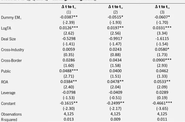
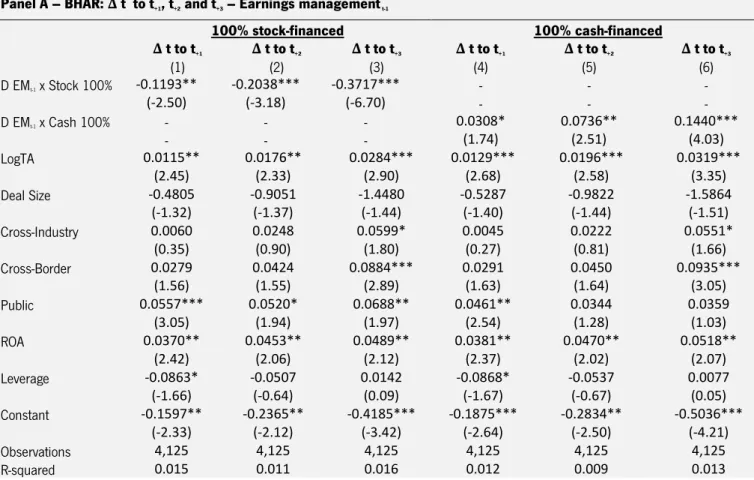
I also find that firms who engaged in earnings management in the year prior to the acquisition, experience a significant decrease in the long-term post-acquisition return performance (BHAR) in average, of 4, 5 and 6 percentage points (UK acquirers experience slightly better returns performance than the rest of the European Union countries). Consistent with this view, firms who engaged in earnings management in the year prior to a stock-financed acquisition, experience a decrease in average of 12, 20 and 37 percentage points in the BHAR from the year of the acquisition to the next 1, 2 and 3 years, respectively.

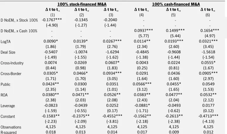
Firms who did not engage in EM in the year prior to a cash-financed acquisition, experience an increase, on average, of 9, 15 and 17 percentage points in the BHAR from the year of the acquisition to the next 1, 2 and 3 years, respectively.

The purpose of this dissertation is to understand if enterprises involved in these earnings manipulation practices have actually achieved what they desired or are simply delaying the sinking of the “ship”. This is a vital topic in finance, as it can cause significant impact on the financial market in general. This dissertation aims to increase the robustness of the knowledge on the use of earnings management in companies involved in M&A.

The remainder of this dissertation is organized into four main parts. After this introduction, the second section - Literature Review - explores the most fundamental studies about earnings management, M&A, and long-term performance. The third section - Data and Methodology - describes the sample used in this research, data sources, empirical methodology, as well as the process of collecting and processing the data necessary to carry out this project. The fourth section - Results - contain the most fundamental analysis made and the respective results. The fifth and last section - Conclusions - covers the most relevant conclusions and the limitations of the dissertation.

5

2. Literature Review and Hypotheses Development

Earnings Management

According to Dechow and Skinner (2000), earnings management, unlike fraud, involves the selection of accounting procedures and estimates that conform to generally accepted accounting practices. Dechow and Skinner (2000) classify the types of earnings management into three, accruals management, real earnings management and fraudulent accounting.

P. Healy and Wahlen (1999) state that earnings management occurs when managers, through legal procedures, change the financial statement, so the investors obtain a different (or incomplete) view of the economic situation of the company.

According to Amat, Blake and Dowds (1999), earnings management consists on the manipulation made on the accountancy information, taking advantage of non-specific rules and possible alternatives that the manager has at his disposal on the different assessment practices used. Levitt (1998) states that managers exploit the flexibility in financial reporting with the objective of meeting the earnings expectations.

The fraudulent accounting involves accounting choices that violate the International Financial Reporting Standards (IFRS)3F

4. Association of Certified Fraud Examiners (2014) mention that

financial statement fraud has a frequency of only 9% (of the total occurrence of occupational fraud4F

5),

but it has a median loss of $1 million (five times higher financial impact than the type of fraud that causes the most financial impact, corruption).

Accordingly to the Transparency International (2015), out of a total of 177 analyzed countries, the EU has 4 countries in the top 5 countries with less Corruption Perceptions Index (CPI)5F

6. This Index

scores range on a scale from 0 (highly corrupt) to 100 (very clean). Accordingly to Transparency International (2015), EU also has 86% of the countries with CPI above 50 (G20 has 47% above 50 and the World average is 57% above 50 CPI).

4 A set of accounting standards developed by the International Accounting Standards Board (IASB), mainly adopted for

the preparation of public company statements (IFRS, 2016).

5 Occupational fraud is classified into three main categories: Asset misappropriation, corruption and financial statement

fraud.

6 According to Perols and Lougee (2011), there is a strong correlation between earnings management and the financial statement frauds. Using a sample of 54 fraud and 54 non-fraud firms, the authors find that fraudulent firms are more likely to have managed earnings in prior years.

Deangelo (1986) and P. Healy (1985) studies, are one of the first in earnings management that address the measurement of discretionary accruals. They state that when firms inflate financial statements by managing their earnings, they increase the generation of accruals income. Dechow et al. (1996) and Lee, Ingram and Howard (1999) argue that companies that increased income accruals in earlier years, must deal with the consequences of the accruals reversal, and most of them commit fraud to offset the reversals.

Beneish (1999) states that increasing discretionary accruals in prior year incomes, leads the company to run out of ways to manage earnings in further years. Thus, managers might opt for fraudulent activities when they are confronted with subsequent earnings reversals and the decreasing flexibility of earnings management.

Real earnings management6 F

7 have also been studied in the last few years, but not in so many

studies. And was done almost exclusively in combination with accruals-based ones (Zarowin, 2015).

Discretionary Accruals and Non-Discretionary Accruals

Earnings management research is essentially focused on the accruals’ analysis (Dechow, Sloan, & Sweeney, 1995). As discretionary accruals are the accruals which can be manipulated, it is how it is measured the earnings management. Splitting the accruals into expected (non-discretionary) and unexpected (discretionary) has a significant role. The most appropriate model for computing discretionary accruals is the Modified-Jones (1991) model, according to the existing literature. Dechow et al. (1995), and Botsari and Meeks, 2008), state that this model is the most suitable to detect earnings management. Besides that, Guay, Kothari, and Watts (1996) present evidence that shows that only the Jones (1991) and Modified-Jones (1991) models appear to provide reliable estimates of discretionary accruals.

7 Moreover, Vladu and Cuzdriorean (2014) state that earnings management studies over the last decade are mostly developed applying accruals-based models. Despite new models being developed and tested by researchers, as mentioned before, they are still based on the accruals model. The ideal goal would be to achieve a model that perfectly detects earnings management. New versions keep being tested, but most are derived from the Jones (1991) model.

According to M. Jones (2011), the accruals represent the non-cash flow elements of the accounts and can often be manipulated by the managers. These accruals represent elements like inventory, depreciation, trade payables and trade receivables.

The total accruals are estimated subtracting the reported accounting earnings by the cash flow from operations. Then are separated into two branches, the discretionary and non-discretionary accruals. Managers can only adjust the discretionary accruals and not the non-discretionary accruals. The discretionary accruals can be manipulated because they are under a certain level of arbitrariness (Jones, 2011). Thus the earnings management is understood as the process by which managers can manipulate the financial statement in order to represent what they wish to have happened or what the investors were expecting (rather than what actually happened) during a certain period.

On the amortization context, a discretionary accrual can be, for instance, a change to the policy for the calculation of the amortization expense by modifying the estimated useful life measurement. The non-discretionary accrual (over which managers do not have control) would be a change to the amortization expense.

Another example of a discretionary accrual can be the increase in inventory, which would incorporate fixed overhead expenses to inventory rather than charging them off as costs. On the other side, the non-discretionary accruals can be the inventory accumulation due to anticipation of increased demand.

Motivations and Consequences of Earnings Management

Jones (2011), argue that there are several reasons that lead managers to adopt practices of earnings management in companies. The main objective is either to cover and benefit the company, or to cover and benefit themselves. In other words, the incentives can be both external and internal factors.

8 Managers tend to manipulate earnings to their benefit when their position is under threat. It can also be used to obtain larger compensation by increasing the value of their equity-based compensation schemes, such as executive stock options (ESO)7F

8. In other words, managers can

improve their (short-term) reputation and extract higher rents if the company continues to show better results year after year.

Another reason for the adoption of earnings management practices is to respond to market expectations. Firms may feel the need to beat the analysts’ forecasts (especially in the case of bad projections). By doing so, firms will create the illusion of having good prospects and increase the confidence of investors. The same type of incentives may exist in situations when the firm is struggling to meet its debt covenants (DeFond & Jiambalvo, 1994; P Healy & Wahlen, 1999) and need additional external financing (Teoh, Welch, & Wong, 1998). Other situations may lead to the practice of earnings management include specific contracts such as bonus plans (J. Gaver, K. Gaver, & Austin, 1995) and specific circumstances such as earnings decreases or losses (Burgstahler & Dichev, 1997).

By analyzing firms under SEC investigations (total 92 firms) between 1982 and 1992, Dechow et al. (1996) state that earnings management behavior lead to a 9% of stock price decline in the two years following the announcement of the earnings management investigation.

In fact, earnings management are not only present in M&A. They are also common in seasoned equity offerings (SEOs) and initial public offerings (IPOs).

Teoh et al. (1998), in relation to SEOs, state the evidence of a relation between earnings management (based on a variation of Modified Jones (1991) model) and the long-run SEO issuer performance. The relation is that the issuers who engage in earnings management have lower post-issue long-run abnormal stock returns and net income. Using as sample, all the seasoned equity issuers from 1976 to 1989 (total 1,265).

Still, Cohen and Zarowin (2010), with a sample of completed US offers over 1987 to 2006 (total 1,551), state that SEO firms engaged in earnings management (based on Jones (1991) model),

8 ESOs gives to an employee (executive) the legal right, but not the obligation, to buy a certain number of shares of the

9 suffer the respective consequences, mainly, the operating underperformance (due the accruals reversal).

More recently, Fauver, Loureiro and Taboada (2015) state the evidence of earnings management (based on Modified Jones (1991) model) on SEOs, using a sample based on EU countries, during the period of 1999 to 2012 (total 1,352). They show the significant increase in crash risk for the issuers that engage in earnings management.

Furthermore, Loureiro and Silva (2015) also state that cross-delisted firms that manipulate earnings (based on Modified Jones (1991) model) prior to an SEO increase the probability of a stock price crash subsequently. In this study, the sample is composed by 583 cross-delisted firms from U.S. stock exchanges markets (38 countries), between 2000 and 2012.

As mentioned before, the presence of earnings management also exists in IPOs. Roosenboom, Van der Goot, and Mertens (2003), with a sample of Dutch IPO firms from 1984 to 1994 (total 64), show that firms with high levels of earnings management (based on Jones (1991) model) tend to exhibit declines in stock returns in the year following the IPOs.

Still, Chiraz and Anis (2013), based on a sample of French IPOs over the period 1999 to 2007 (total 139), state that the firms associated with earnings management (based on Modified Jones (1991) model) in the IPO process tend to suffer from poor returns and delist8F

9 due the performance

failure subsequently to the IPO.

Also, Bao, Chung, Niu and Wei (2013), suggest that IPO firms manipulate their earnings (based on Modified Jones (1991) model) in the IPO year to inflate reported earnings. This study is based on a sample of US IPO firms from 1990 to 2007 (total 1,014).

More recently, Alhadab, Clacher and Keasey (2015), with a sample based on UK IPO firms from 1998 to 2008 (total 570), argue that these firms engaged in earnings manipulation (based on Modified Jones (1991) model) during the IPO year. Besides that, the firms who present higher levels of earnings management have higher probability of IPO failure and lower survival rates in subsequent periods.

9 Delisting includes violating regulations, and/or failing to meet financial specifications (minimum share price, minimum

10 Cases with evidence of earnings management around M&A are presented in the next section in detail.

Earnings Management on Mergers and Acquisitions

According to the literature, it is known that earnings management are present in some M&A. It is particularly prevalent when stock is used as a payment, which may entice the acquirer to manipulate its stock prices (Botsari & Meeks, 2008; Erickson & Wang, 1999; Rahman & Bakar, 2003). The acquiring firm has an incentive to increase earnings preceding to the merger, to raise the market price or the appraised price9F

10 of its stock. Also, that the companies do that by

aggressively using discretionary accruals to temporarily inflate the purchasing power of their stock, therefore reducing the effective cost of the acquisition (Erickson & Wang (1999).

In the context of M&A, Erickson and Wang (1999), is the first to test for earnings management in acquiring firms involved in stock-financed M&A, recognizing the possible incentives for firms that conduct stock-financed acquisitions to manipulate their earnings (based on a model developed by themselves, but based on Jones (1991) model). They state that when an acquisition is stock-financed, the exchange ratio (number of shares given by acquirer for each share of the target company), is inversely related to the acquiring firm’s stock price. In their study, with a sample of 55 stock-financed acquisitions occurring between 1985 and 1990 in US, state that firms conducting stock-financed acquisitions do manage their earnings upwards before their acquisitions. In contrast, they report no evidence of earnings management in a control group of 64 cash-financed acquisitions.

Heron and Lie (2002) come to a different conclusion from Erickson and Wang (1999). They sustain that acquiring firms, prefer to pay for their acquisitions with stock when those are overvalued, and to pay with cash when their stocks are undervalued. However, with a sample of US market’s M&A from 1985 to 1997 (total 859, where around 50% were entirely stock-financed), they find no evidence that acquirers engage in earnings management (based on Modified-Jones (1991) model) prior to acquisitions. They argue that this difference to Erickson and Wang, 1999 could be due to different samples or different procedures estimating the accruals (different models).

10 The appraised stock value is defined by a third party company, usually an investment bank, engaged by the target

11 The remaining literature focusing on stock-financed acquisitions is consistent with Erickson and Wang (1999). The results from Rahman and Baka (2003) suggest that stock-financed acquisitions manage earnings upwards in the year prior to the acquisition (based on Jones (1991) and Modified-Jones (1991) models). They use a total of 120 Malaysian M&A over the period 1991 to 2000 as a sample.

Louis' (2004) study includes 373 M&A made between 1992 and 2000 of US companies, where 236 (63% of total) are only stock-financed. The conclusions suggest that earnings management (based on a variation of Jones (1991) model) are positive and statistically significant for acquirers that made acquisitions with stock previous to the acquisition; second, discretionary accruals are insignificant for acquirers that made acquisitions with cash.

Botsari and Meeks (2008) with a sample based on the UK M&A between 1997 and 2001 (total of 176), suggest the presence of earnings management (based on Jones (1991) model and Modified Jones (1991) model) on stock-financed acquisitions.

More recently, Vasilescu and Millo (2016) state that in a sample of 229 M&A occurred in UK between 1990 to 2008, firms in general engage in earnings management (based on Modified Jones (1991) model) prior to M&A. This study does not make a distinction about the method of payment, but instead, it tests if earnings management are more evident in industry or cross-border M&A. The results suggest that geographic diversification is linked to higher earnings management. However, the results are not statistically significant.

Earnings management appears to be quite common based on previous studies. Despite that, acquiring firms may choose not to do it. Agency theory states that for earnings management to occur, the cost of not doing it must exceed the cost of doing it (Watts & Zimmerman, 1990). What is observed is that most studies show evidence for the aggressive use of earnings management.

Post-Acquisition Performance on Mergers and Acquisitions

In relation to post-acquisition performance in M&A, as mentioned before, an M&A can turn out to be profitable and beneficial to the firms, as well as devastating and detrimental. If the acquiring company engages in earnings management prior to the acquisition, it can generate serious problems to its post M&A performance. Some studies argue that the method of payment used by the acquirer companies is directly related to the companies having been engaged or not in earnings management prior to the acquisition. Based on the literature, both long-term post-operating

12 performance as well as term return performance (BHAR) are two alternatives to test the long-term post-acquisition performance of the M&A.

Post-Acquisition Operating Performance

In relation to the long-term post-operating performance in M&A, Hotchkiss and Mooradian (1998), state the evidence of significant positive changes on the testing sample, comparing to the control sample (non-bankrupt targets), which shows no significant improvements from the year prior to the acquisition to years +1 and +2. However, no distinction from stock, or cash acquisitions was made. The target firms are bankrupt targets10F

11, the total M&A on their sample is 55, occurred in US, during

1979 and 1992. Operating performance scaled by sales (also scaled by assets, which presented similar conclusions) is the method which they pointed out as being the most appropriate methodology to test the operating performance in M&A.

Ghosh (2001) with a sample based on 315 (147 paid in cash, 111 pain in stock, and the remaining 57 with a mix of both) M&A occurred in US between 1981 and 1995, find no evidence that operating performance increase following an M&A comparing with benchmark composed by firms matched by pre-acquisition performance and size. However, the performance is significantly higher in cash acquisitions and stock experience a decline following an M&A. The method used is operating income scaled by assets

Heron and Lie (2002), state that neither the cash nor stock payment methods convey information about the future operating performance of the acquirers. The method used is operating income scaled by sales and operating income scaled by assets. The acquirers that pay with stock, outperform their industries when compared to the ones that pay with cash, but only by slightly larger margins, however. Also, the authors argue that acquirer firms exhibit higher levels of operating performance when buying with stock, and that they continue to exhibit superior operating performance post-acquisition, than the control firms (with similar pre-acquisition operating performance). In this study, the sample is composed by 859 US acquisitions (342 paid in cash, 427 pain in stock, and the remaining 90 with a mix of both) between 1985 and 1997.

Still in relation to operating performance, Kruse, Park and Suzuki (2007), with a sample of 69 M&A from Japan between 1969 and 1999, state the evidence of improvements in operating

13 performance for their entire sample (from year -5 and -1 to +1 and +5), however no distinction from stock, or cash acquisitions was made. The method used is operating income scaled by sales and operating income scaled by assets.

More recently, (Rao-Nicholson, Salaber, & Cao, 2016) suggest that in their sample of 57 M&A occurred in ASEAN11F

12 countries between 2001 to 2012, the operating performance tends to decline

in the 3 years following an M&A. The method used is operating income scaled by sales and operating income scaled by assets. And consistent with Heron and Lie (2002) and Kruse et al. (2007) the acquisitions outperform their industries their respective industry benchmark before and after the M&A. In this study, no distinction from stock or cash acquisitions was made.

According to Barber and Lyon (1996), scaling the operating income by sales is the most appropriate measure of operating performance in M&A. Heron and Lie (2002) state that this method should be immune against the method of accounting12F

13 or method of payment

13F

14 on the M&A, so researchers

tend to use this methodology to test the operating performance in M&A.

Buy and Hold Abnormal Return

On the long-term return performance, Agrawal, Jaffe and Gershon (1992), find statistically significant decrease in their sample (they do not distinguish from stock, or cash acquisitions), a loss of about 10% over the 5 years post-acquisition. The used sample is composed by 937 M&A which occurred in US during 1955 to 1987.

Also, in relation to long-term return performance, Mitchell and Stafford (2000) analyze the BHAR of M&A involved companies 3 years after the acquisition. The analyzed sample is composed by 4,911 US events (2,421 SEOs and 2,193 acquisitions), from 1958 to 1993. The result points to the existence of underperformance by the M&A, comparing to the benchmark portfolios (25 value-weight non-rebalanced14F

15 portfolios). However, they find that stock-financed acquisitions perform

worse than the cash-financed ones.

12 ASEAN - Association of Southeast Asian Nations, has 10 member states, Brunei, Cambodia, Indonesia, Laos,

Malaysia, Myanmar, Philippines, Singapore, Thailand and Vietnam.

13 The methods of accounting used in M&A is usually Pooling of Interests or Purchase Method. The main difference is

that Purchase Method allow the company to charge for goodwill (reputation of the business). Using the Pooling of Interests the company is evaluated by book value rather than market value.

14 The method of payment used in M&A is usually cash, stock or a combination of both.

14 Louis' (2004) study includes 373 mergers made between 1992 and 2000 of US companies, where 236 (63% of total) are exclusively stock-financed. Its results suggest that the long-term return performance (BHAR) is negative and statistically significant for the stock-financed acquisitions, and positive and statistically significant for the cash-financed acquisitions on the year +1, +2 and +3 following the acquisition.

Long-term performance is still a controversial subject. It is a topic that still has many branches, each with its limitations, which is why researchers are still split on different ways to measure it. That makes it important to analyze the context and the sample used, in order to choose the most appropriate performance measure.

Hypotheses to test

The literature referred above, are essentially based on the US market or in a specific country, and it shows that, a stock-financed acquisition is more likely to use earnings management to inflate the purchasing power of the company’s stocks. Thus, for the first part of this dissertation, I formulate the following testable hypothesis:

H1: The likelihood of a stock-financed acquisition is higher when the acquiring firm engaged in earnings management prior to the acquisition announcement.

Besides the importance of knowing whether a company was engaged in earnings management prior to the acquisition announcement, it is also important to know if that practice reverts in the long-run and leads to poor post-deal operating and/or return performance. As contested in the most of cases in the literature review, is expected that acquirers experience normal long-term post-acquisition performance around the cash-financed post-acquisitions, and negative around the stock-financed acquisitions. Based on this expectation, for the second part of this dissertation, I formulate the following testable hypothesis:

H2: The long-term post-acquisition performance of stock-financed acquisitions should be weaker in cases when the acquiring company engaged in earnings management prior to the acquisition.

15

3. Data and Methodology

Data and Sample

The sample used in this research comprises European Union acquirers that were involved in M&A between 2000 and 2014.

This study intends to fill a gap in the literature when it comes to its earnings management around M&A in European Union countries. As mentioned in the literature review, most studies focused on earnings management in M&A are analyzing the US market (Erickson & Wang, 1999; Heron & Lie, 2002) and UK (Botsari & Meeks, 2008; Vasilescu & Millo, 2016). Another objective of this study is to analyze the post-acquisition performance in M&A, which once again, as far as I know, no other study does for EU countries (see section 2.2).

Following the literature (e.g., Bertrand & Zitouna, 2008; Moeller, Schlingemann, & Stulz, 2004; Rossi & Volpin, 2004) an acquisition is defined as a target when the percentage owned before the acquisition is less than 50% and after the acquisition is higher than 50%.

Also, although the acquiring companies are restricted to EU nations, no restriction is imposed to the target companies. All the deal specific data are from Thomson Financial’ Securities Data Company’s (SDC) Platinum Database. The necessary financial statement data (firm specific variables) to compute the earnings management and the post-operating performance are from Thomson Financial’ DataStream/ WorldScope Database, in dollar currency.

For a firm to be included in the sample, I follow the existing literature (e.g., Botsari & Meeks, 2008; Heron & Lie, 2002; Louis, 2004; Loureiro & Silva, 2015; Loureiro & Taboada, 2015; Vasilescu & Millo, 2016), and apply the following criteria:

 The M&A announcement occurs between January 1st of 2000 and December 31st of 2014

(15 years);

 The data must have the accounting information necessary to compute the discretionary accruals and long-term post-acquisition performance (firm specific variables from 1998 to 2015 in order to compute lead and lagged variables);

 The acquirer is established in one of the European Union countries (28 countries), no restriction about the target;

 The observations gathered from SDC have to include the Sedol of the acquirer;  The transaction is completed, and the M&A deal value was above $1 Million;

16  The percentage owned by acquirer after the M&A is at least 50%;

 Only assume the first acquisition for each acquirer in the same year (to avoid clustered observations);

 Different target and acquirer companies, to avoid situations in which the acquirer is acquiring back his company (self-acquisitions);

 The Percentage of Stock and/or Percentage of Cash variables were not empty, because it is not possible to recover that information (explained in Appendix A);  Exclude acquirers from the financial industry due to their unique disclosure requirements

(SIC codes15F

16 between 6000 and 6999)

16F

17.

As the interval between M&A announcement dates and effective dates is typically several months long, and since the effective date is not always available, the announcement date is assumed as the completion date, a common practice in the literature. To mitigate the impact of outliers on the sample, all variables are winsorized at 1% percentile and 99% percentile (Botsari & Meeks, 2008; Kruse et al., 2007; Louis, 2004; Loureiro & Silva, 2015). Also, to make observations more comparable over time, all the monetary variables were adjusted to real values according to the Consumer Price Index 2014 USD prices17F

18 (Bureau of Labor Statistics, 2015).

The total M&A deals collected from SDC was 46,467. The next step was to merge it with the data from WorldScope. The variables are described in Appendix A. After merging, there were 2763 acquirers, who made 5,982 acquisitions. However, the sample size may vary accordingly to each estimation procedures.

Over 58% of the deals involve acquirers and targets with the same 2-digit SIC code and over 47% with the same 3-digit SIC code. Therefore, only half of the M&A are between targets and acquirers of different industries (conglomerates). Also, around 52% of the acquisitions involve targets and acquirers located in the same country.

It is important to mention that in my sample more than 300 observations do not have the complete data about the amount of percentage of stock or cash used to finance the acquisition. In this cases the sum of the two percentages of cash and stock used to finance the M&A do not totalize 100%

16 SIC is the Standard Industrial Classification – for the left to right, the 1st digit identifies the division, the 2nd digit

identifies the major group, the 3rd digit identifies the industry group and the 4th digits identifies the industry.

17 The 6000-6999 group (financial sector) are excluded because they have different regulations (e.g., Botsari & Meeks,

2008; Louis, 2004; Loureiro & Taboada, 2015).

18 I chose the Consumer Price Index for all urban consumers (CPI-U), because it covers more population, around 87%,

17 (which is expected, since it is the payment for the acquisition as a whole). In others observations the total sum of the method of payment were also lower than 100%. However, it also makes sense to in some cases it does not totalize 100% due some deals that can be made (e.g., cases in which payments in installments were agreed).

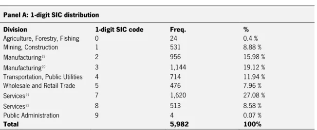
Table 1 provides a distribution of my sample per 1-digit SIC (Panel A), per year and payment method (Panel B), and per acquirer country (Panel C). Note that in the Panel A, the SIC codes between 6000 and 6999 are not present due to regulation differences in relation to other industries. In the Panel B, I present the time-series of my sample split by the year of announcement and method of payment.

Also, as mentioned before, the M&A waves are visible in the Panel B. The period of 1992 to 2002 is the 5th M&A wave. The decline of M&A activity in the year of 2000 to 2001 (decrease of 4

percentage points) and of 2001 to 2002 (decrease of 1.80 percentage points) can be observed. Despite it being a low increase, there was an growth in M&A activity from 2003 to 2007, the 6th

M&A wave (Kummer & Steger, 2008). 100% cash payments are more than 50% of my sample and 100% stock payment are only around 12%. Panel C, it is noticeable how the presence of the UK is very evident in M&A, since around 57% of the sample is UK acquirers. This is a possible justification to the existence of many studies developed in this country.

Table 1 - Data Distribution

Panel A: 1-digit SIC distribution

Division 1-digit SIC code Freq. %

Agriculture, Forestry, Fishing 0 24 0.4 %

Mining, Construction 1 531 8.88 %

Manufacturing18F

19 2 956 15.98 %

Manufacturing19F

20 3 1,144 19.12 %

Transportation, Public Utilities 4 714 11.94 % Wholesale and Retail Trade 5 476 7.96 % Services20F 21 7 1,620 27.08 % Services21F 22 8 513 8.58 % Public Administration 9 4 0.07 % Total 5,982 100%

19 SIC codes between 20 and 29 include food, tobacco, textile, furniture, chemicals, petroleum, etc. 20 SIC codes between 30 and 39 include leather, stone, glass, metal, electronic, computer equipment, etc. 21 SIC codes between 70 and 79 include personal, business, automotive, hotels, camps, etc.

18

Panel B: M&A Time distribution and Payment method

Full Sample 100% Cash Payment 100% Stock Payment Mixed Payment

Year Total % Δ% t to tt-1 N % of Total N % of Total N % of Total

2000 739 12.4% 318 5.3% 143 2.4% 278 4.6% 2001 505 8.4% -4.00% 228 3.8% 70 1.2% 207 3.5% 2002 397 6.6% -1.80% 238 4.0% 43 0.7% 116 1.9% 2003 315 5.3% -1.30% 164 2.7% 43 0.7% 108 1.8% 2004 361 6.0% +0.70% 169 2.8% 46 0.8% 146 2.4% 2005 486 8.1% +2.10% 238 4.0% 52 0.9% 196 3.3% 2006 508 8.5% +0.40% 249 4.2% 57 1.0% 202 3.4% 2007 537 9.0% +0.50% 282 4.7% 46 0.8% 209 3.5% 2008 373 6.2% -2.80% 206 3.4% 36 0.6% 131 2.2% 2009 254 4.2% -2.00% 130 2.2% 33 0.6% 91 1.5% 2010 324 5.4% +1.20% 168 2.8% 37 0.6% 119 2.0% 2011 315 5.3% -0.10% 179 3.0% 30 0.5% 106 1.8% 2012 285 4.8% -0.50% 158 2.6% 32 0.5% 95 1.6% 2013 268 4.5% -0.30% 136 2.3% 23 0.4% 109 1.8% 2014 315 5.3% +0.80% 160 2.7% 33 0.6% 122 2.0% Total 5,982 3,023 50.5% 724 12.1% 2,235 37.4%

Panel C: M&A Place distribution

Acquirer Country Freq. Percent Cum.

United Kingdom 3,413 57.05% 57.1% France 463 7.74% 64.8% Sweden 462 7.72% 72.5% Germany 305 5.10% 77.6% Italy 204 3.41% 81.0% Netherlands 192 3.21% 84.2% Finland 177 2.96% 87.2% Ireland-Rep 143 2.39% 89.6% Spain 137 2.29% 91.9% Poland 114 1.91% 93.8% Denmark 96 1.60% 95.4% Belgium 91 1.52% 96.9% Greece 49 0.82% 97.7% Austria 36 0.60% 98.3% Portugal 27 0.45% 98.8% Luxembourg 25 0.42% 99.2% Cyprus 18 0.30% 99.5% Czech Republic 10 0.17% 99.7% Slovenia 8 0.13% 99.8% Hungary 6 0.10% 99.9% Lithuania 2 0.03% 99.9% Romania 2 0.03% 100.0% Croatia 1 0.02% 100.0% Estonia 1 0.02% 100.0% Total 5,982 100%

Panel A shows the distribution by 1-digit SIC. Panel B shows the distribution by year of announcement of M&A and by method of payment. Panel C Stock payment refers to acquisitions which were completely financed with stock. Cash payment refers to acquisitions which were completely financed with cash. Mixed payment refers to acquisitions which were financed with stock and cash. Around 50% of the sample were acquisitions cash-financed (3,023 M&A) and 12% were stock-financed (724 M&A). 28 countries belong to EU, although only 24 countries are present in my sample (Panel C). Malta, Latvia, Slovakia and Bulgaria were excluded from my sample due to they fail to meet some necessary requirements (requirements is presented in the next section).

19

Methodology

Calculation of the Earnings Management

According to the existing literature, the most appropriate methodology to measure earnings management is to compute total discretionary accruals (Teoh et al., 1998; Dechow et al., 1995; Botsari & Meeks, 2008). Among the various discretionary accrual models, the Jones (1991) and the Modified-Jones (1991) models are the ones that perform the best (Dechow et al., 1995). Also, Botsari et al. (2008) state that the Modified-Jones (1991) model is better to detect earnings management, even the more subtle cases.

According to Vladu and Cuzdriorean (2014) studies about earnings management over the last decade are mostly developed applying accruals-based models. Despite new models being developed and tested by researchers, they are still based on the Jones (1991) model.

The main goal is to achieve a model that perfectly detects earnings management. That’s why new versions are always being tested. Real earnings management have also been studied in the last few years, but only in a few studies. And that was done with accruals-based models studies, or almost exclusively in combination with accruals-based ones.

3.2.1.1. Discretionary Total Accruals

The Jones (1991) model (and the modified version) is a cross-sectional model. I use firms in the same country and in the same 1-digit SIC code to estimate the total discretionary accruals. I use at least 10 observations in each 1-digit SIC group per year to obtain more reliable parameter estimates (e.g., Erickson & Wang, 1999; Jeter & Shivakumar, 1999; J. Jones, 1991; Teoh et al., 1998). On my study, I only apply the modified version22F

23 since it produces similar results as other

versions, as documented in previous studies (e.g., Botsari & Meeks, 2008; Dechow et al., 1995; Rahman & Bakar, 2003).

According to the previous literature (e.g., Dechow et al., 1995; Heron & Lie, 2002; Kothari, Leone, & Wasley, 2005; Loureiro & Silva, 2015) the total value of discretionary accruals is used as a proxy for earnings management. It suggests that managers distort reported data in case of high values of discretionary accruals. In other words, they manipulate the financial reports, masking the firms’

23 The only change relatively to the original model is that the change in revenues is adjusted for the change in receivables

20 true economic performance (Dechow & Skinner, 2000). Sloan (1996), refers to discretionary accruals as a “measure of financial reporting opacity because it masks some information about the firm’s fundamentals” (as cited in Loureiro and Silva, 2015, p.3). All variables in the accruals model are scaled by lagged total assets to reduce heteroskedasticity (e.g., Erickson & Wang, 1999; J. Jones, 1991; Teoh et al., 1998).

To start, the following regression is estimated for a 1-digit SIC group per country and year. The Modified-Jones (1991) model is the following one and is the model that I use in this dissertation (J. Jones, 1991): 𝑇𝑜𝑡𝐴𝑐𝑐_𝑖𝑡 𝑇𝐴_𝑖𝑡−1 = 𝛼 1 𝑇𝐴_𝑖𝑡−1+ 𝛽1 Δ𝑅𝐸𝑉_𝑖𝑡− Δ𝑅𝐸𝐶_𝑖𝑡 𝑇𝐴_𝑖𝑡−1 + 𝛽2 𝑃𝑃𝐸_𝑖𝑡 𝑇𝐴_𝑖𝑡−1+ 𝜀𝑖,𝑡, (1)

Where, for firm i in year t:

TotAcc = is the change in non-cash current assets minus the change in net income and cash flow from operations;

ΔREV = revenues in year t less revenues in year t-1;

ΔREC = accounts receivable in year t less revenues in year t-1;

PPE = gross property plant and equipment; TAit-1 = Total assets at t-1.

Then it is necessary to estimate the nondiscretionary accrual, obtained using estimates from the regression above (2): 𝑁𝐷𝑇𝐴𝐶𝐶_𝑖𝑡 = 𝛼̂ 1 𝑇𝐴𝑖𝑡−1 + 𝛽̂ ₁ Δ𝑅𝐸𝑉𝑖𝑡− Δ𝑅𝐸𝐶𝑖𝑡 𝑇𝐴𝑖𝑡−1 + 𝛽̂ ₂ 𝑃𝑃𝐸𝑖𝑡 𝑇𝐴𝑖𝑡−1 (2)

Next, I compute the discretionary accruals (DISCACC). As mentioned above, this is what is used to analyze if a company is practicing earnings management or not.

𝐷𝐼𝑆𝐶𝐴𝐶𝐶𝑖𝑡 =

𝑇𝑂𝑇𝐴𝐶𝐶𝑖𝑡

𝑇𝐴𝑖𝑡−1

− 𝑁𝐷𝑇𝐴𝐶𝑖𝑡 (3)

The variable codes23F

24 are indicated in Appendix A 3.2.1.2. Probit Multivariate Analysis

The first hypothesis of this study is tested using a probit model. In the first hypothesis I test if the likelihood of a stock-financed acquisition is higher when the acquiring firm engaged in earnings

24 WorldScope database and Compustat database (the Compustat variable codes are equivalent ones to the

21 management prior to the acquisition announcement. I test this hypothesis using various specifications of the following probit regression:

𝐷𝑆𝑡𝑜𝑐𝑘_𝑖𝑡 = 𝛿₀+ 𝛿₁𝐸𝑀_𝑖𝑡−1+ 𝛿₂𝑀𝑇𝐵_𝑖𝑡−1+ 𝛿₃𝑅𝑂𝐴_𝑖𝑡−1+ 𝛿₄𝐿𝑒𝑣𝑒𝑟𝑎𝑔𝑒_𝑖𝑡−1

+ 𝛿5𝐷𝑒𝑎𝑙𝑆𝑖𝑧𝑒𝑖𝑡+ 𝛿6𝐶𝑟𝑜𝑠𝑠𝐵𝑜𝑟𝑑𝑒𝑟𝑖𝑡+ 𝛿7𝐶𝑟𝑜𝑠𝑠𝐼𝑛𝑑𝑢𝑠𝑡𝑟𝑦_𝑖𝑡 + 𝜏𝑖𝑡

(4)

Where, for firm i in year t:

DStock = Dummy variable, 1 if it is a 100% stock-financed acquisition, 0 otherwise24F

25_;

EM = Earnings Management25 F

26;

MTB = Market to Book26 (Market Value / Book Value Equity);

ROA = Return on Assets26 (Net Income / Total Assets);

Leverage = Leverage26 (Total Debt / Total Assets);

DealSize = Relative Deal Size (Value of Transaction / Total Assetst-1);

CrossBorder = Dummy variable, 1 if it is a cross-border acquisition, 0 otherwise; CrossIndustry = Dummy variable, 1 if it is a cross-industry acquisition, 0 otherwise; τ = Error term.

In order to perform a more robust analysis, I also test the reverse of Hypothesis 1, by estimating a similar probit model to the one presented above, where the dependent variable now identifies acquisitions that were fully paid in cash. Thus, I estimate the following model:

𝐷𝐶𝑎𝑠ℎ_𝑖𝑡 = 𝛿₀+ 𝛿₁𝐸𝑀_𝑖𝑡−1+ 𝛿₂𝑀𝑇𝐵_𝑖𝑡−1+ 𝛿₃𝑅𝑂𝐴_𝑖𝑡−1

+ 𝛿₄𝐿𝑒𝑣𝑒𝑟𝑎𝑔𝑒_𝑖𝑡−1+ 𝛿₅𝐷𝑒𝑎𝑙𝑆𝑖𝑧𝑒_𝑖𝑡+ 𝛿₆𝐶𝑟𝑜𝑠𝑠𝐵𝑜𝑟𝑑𝑒𝑟_𝑖𝑡

+ 𝛿7𝐶𝑟𝑜𝑠𝑠𝐼𝑛𝑑𝑢𝑠𝑡𝑟𝑦_𝑖𝑡 + 𝜏𝑖𝑡

(5)

Where, for firm i in year t:

DCash = Dummy variable, 1 if it is a 100% stock-financed acquisition, 0 otherwise26F

27;

EM = Earnings Management27 F

28;

MTB = Market to Book28 (Market Value / Book Value Equity);

ROA = Return on Assets28 (Net Income / Total Assets);

Leverage = Leverage28 (Total Debt / Total Assets);

DealSize = Relative Deal Size (Value of Transaction / Total Assetst-1);

CrossBorder = Dummy variable, 1 if it is a cross-border acquisition, 0 otherwise; CrossIndustry = Dummy variable, 1 if it is a cross-industry acquisition, 0 otherwise; τ = Error term.

The variable codes28F

29 are indicated in Appendix A

25 I also test different percentages of stock used to finance the acquisitions, e.g. 1 = 100% stock; 1 = 75% stock; 1 =

50% stock, 0 = otherwise.

26 Variable computed in previous year to the announcement year.

27 I also test different percentages of amount of cash used to finance the acquisitions, e.g. 1 = 100% cash; 1 = 75%

cash; 1 = 50% cash, 0 = otherwise.

28 Variable computed in previous year to the announcement year.

29 WorldScope database and Compustat database (the Compustat variable codes are equivalent ones to the

22

Calculation of the Long-Term Post-Acquisition Performance

Firm performances are already investigated in many existing studies, tough that is still controversial between the existing studies, as mentioned above. As Mitchell and Stafford (2000, p.288) state, “(…) measuring long-term abnormal performance is treacherous”. So, in order to obtain a more robust result, I test two different performance metrics to analyze the long-term post-acquisition performance of acquirers involved in M&A:

 Long-term operating performance  Long-term return performance

In both analysis, I also take into account the three years after the announcement. For operating performance, I also analyze the two years preceding the M&A (totaling a 5-year window).

3.2.2.1. Post-Acquisition Operating Performance

Operating income is considered an official financial income measure under the International Financial Reporting Standards (IFRS) (PriceWatersHouseCoopers, 2007). According to Barber & Lyon, 1996; Hotchkiss & Mooradian, 1998; Kruse et al., 2007, scaling the operating income by sales is the most appropriate measure of operating performance in M&A. So, the first method I use to analyze the post-operating performance is scaling the operating income by sales (Barber & Lyon, 1996; Heron & Lie, 2002; Hotchkiss & Mooradian, 1998; Loureiro & Taboada, 2015).

Although, to provide more robustness, some studies also opt to analyze the operating performance scaling the operating income by assets (Heron & Lie, 2002; Hotchkiss & Mooradian, 1998; Kruse et al., 2007; Rao-Nicholson et al., 2016). Thus, I also test the operating performance scaling the operating income by assets. The variables are defined in Appendix A.

I also follow the literature (e.g., Heron & Lie, 2002; Hotchkiss & Mooradian, 1998; Loureiro & Taboada, 2015) to control for different industries and factors that may affect the operating performance. I compute country-, year-, and the industry-adjusted29F

30 operating performance for each

acquirer.

30 I subtract the median (and also do the same process subtracting the mean, but the most appropriate way is

subtracting the median (e.g., Heron & Lie, 2002; Hotchkiss & Mooradian, 1998; Loureiro & Taboada, 2015)) of operating performance of firms in the same country, same year and same industry (2-digit SIC code).

23 For a control sample, I use the aggregation of the mean (or median) of the operating income to sales ratio by group (the group consist in firms of the same industry (2-digit SIC code), country and year of acquisition). I use all the companies involved in M&A in EU during the period of 2000 and 2014.

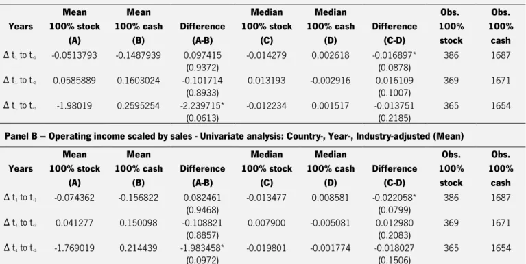
Then I use parametric t-statistics (to test the means) and non-parametric Wilcoxon rank-sum z-statistics (to test the medians), to see if the difference between groups (stock-financed and cash-financed) is significant. So, the steps I use to test the operating performance are the following:

 Compute country-, year-, and industry-adjusted operating performance by taking the difference between the acquirer’s operating income to sales ratio, minus the median/mean ratio of the same acquirer’s country, year of acquisition and industry (2-digit SIC code);

 Compute changes in adjusted-operating performance from 2 years prior to 3 years after the deal;

 Test the univariate differences in means (t-statistics) and medians (Wilcoxon rank-sum z-statistics) between the groups of 100% stock-financed and 100% cash-financed.

3.2.2.2. Buy-and-Hold Abnormal Returns Post-Acquisition

To analyze the post-acquisition long-term return performance of the M&A, I follow previous studies (Agrawal et al., 1992; Louis, 2004; Mitchell & Stafford, 2000), and opt for the buy-and-hold abnormal returns (BHAR) model.

The buy-and-hold abnormal returns method is widely used in the long-run performance analysis. Also, this method is known as a precise measure of investor experience since it captures real investors’ returns experience over a period of time (Barber & Lyon, 1997). It requires analysis over different periods of time in order to produce robust conclusions, since the abnormal performance may occur only in the first year or first 3 years and it might lead to take conclusions too soon (Mitchell & Stafford, 2000).

The buy-and-hold abnormal return is defined as the expected return on a buy-and-hold investment in a sample firm at specific time (I start 1 week after the M&A to 1, 2 and 3 years following it to test if the firm outperform the benchmark) minus the return on a buy-and-hold investment in the benchmark (equally weighted market index of country):

𝐵𝐻𝐴𝑅_𝑖 = ∏(1 + 𝑅_𝑖,𝑡) − 𝑇 𝑡=1 ∏(1 + 𝑅_{𝑏𝑒𝑛𝑐ℎ𝑚𝑎𝑟𝑘,𝑡}) 𝑇 𝑡=1 (6) Where,

24 Ri,t = Weekly return of firm i in week t;

Rbenchmark,t = Weekly return of the market index of country i in week t.

As stated in some studies (e.g., Kothari & Warner, 2007; Mitchell & Stafford, 2000), the main concern about this method is that it assumes that the corporate event’s abnormal returns are independent. However, some events may not be completely random and, more importantly, even if they are there may be some overlapping across observations on the time period for which BHAR are calculated. This means that a positive cross-correlation on abnormal returns is possible. In an attempt to mitigate this problem, an alternative approach, I cluster the standard errors of the regression at the year and country-year levels.

Besides the main problem of BHAR mentioned above, Barber and Lyon (1997) and Kothari and Warner (1997) also mention other issues that can produce biased estimates using the BHAR approach. They point three possible causes, one is the new listing bias. This happens because the sample used in the studies usually hold a long post-event history of returns, while the firms that constitute the reference portfolio usually include all firms (including the new firms that began subsequent to the event month). The second problem is the rebalancing of benchmark portfolio, which is due the compound returns of the reference portfolio (for example, the equally weighted market index is usually calculated assuming generally monthly rebalancing). Relatively to the sample firms, it is compounded without rebalancing. The third problem is the skewness of multi-year, this is due the positive skewness observed in the long-run abnormal returns.

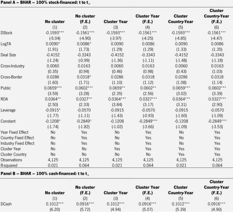
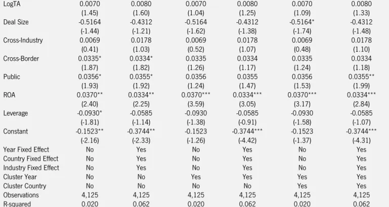
The most complete regression used is the one presented below (7).

𝐵𝐻𝐴𝑅 = 𝛼0+ 𝛼1𝐷𝑆𝑡𝑜𝑐𝑘𝑖 + 𝛼2𝐿𝑜𝑔𝑇𝑜𝑡𝐴𝑠𝑠𝑒𝑡𝑠_𝑖+ 𝛼3𝐿𝑒𝑣𝑒𝑟𝑎𝑔𝑒_𝑖 + 𝛼4𝑅𝑂𝐴𝑖 + 𝛼₅𝐷𝑒𝑎𝑙𝑆𝑖𝑧𝑒_𝑖+ 𝛼₆𝐶𝑟𝑜𝑠𝑠𝐵𝑜𝑟𝑑𝑒𝑟_𝑖 + 𝛼₇𝐶𝑟𝑜𝑠𝑠𝐼𝑛𝑑𝑢𝑠𝑡𝑟𝑦_𝑖

+ 𝛼₈𝑃𝑢𝑏𝑙𝑖𝑐_𝑖+ 𝜀_𝑖

(7)

Where, for firm i

BHAR = Buy-and-hold abnormal returns;

DStock = Dummy variable, 1 if it is a 100% stock-financed acquisition, 0 otherwise; LogTotAssets = Logarithm of Total Assets;

Leverage = Leverage (Total Debt / Total Assets);

ROA = Return on Assets (Net Income / Total Assets);

DealSize = Relative Deal Size (Value of Transaction / Total Assetst-1); CrossBorder = Dummy variable, 1 if it is a cross-border acquisition, 0 otherwise; CrossIndustry = Dummy variable, 1 if it is a cross-industry acquisition, 0 otherwise; Public = Dummy variable, represent a Public target firm if 1, and 0 otherwise; ε = Error term.