U
Un
n
E
SCOLAMestrado em Modelação Estatística e Análise de Dados
Especialização em Modelação Estatística e Análise de Dados
Modelling catch and mortality rates of blue shark captured by the
Portuguese longline fleet in the Atlantic Ocean
“Modelação de taxas de captura e mortalidade de tintureira capturad
pela frota Portuguesa de palangre de superfície
Professor Doutor
Doutor Miguel Neves dos Santos
n
n
iv
i
ve
er
r
si
s
id
d
ad
a
de
e
d
d
e
e
É
Év
vo
or
r
a
a
SCOLA DEC
IÊNCIAS ET
ECNOLOGIAem Modelação Estatística e Análise de Dados
em Modelação Estatística e Análise de Dados
Dissertação
ling catch and mortality rates of blue shark captured by the
Portuguese longline fleet in the Atlantic Ocean
Modelação de taxas de captura e mortalidade de tintureira capturad
pela frota Portuguesa de palangre de superfície no Oceano Atlântico
Rui Pedro Andrade Coelho
Orientador:
Doutor Paulo Jesus Infante dos Santos, Univ. Évora
Co-Orientador:
Doutor Miguel Neves dos Santos, IPMA, I.P.
2013
em Modelação Estatística e Análise de Dados
em Modelação Estatística e Análise de Dados
ling catch and mortality rates of blue shark captured by the
Portuguese longline fleet in the Atlantic Ocean
Modelação de taxas de captura e mortalidade de tintureira capturada
no Oceano Atlântico”
Mestrado em Modelação Estatística e Análise de Dados
Especialização em Modelação Estatística e Análise de Dados
Dissertação
Modelling catch and mortality rates of blue shark captured by the
Portuguese longline fleet in the Atlantic Ocean
“Modelação de taxas de captura e mortalidade de tintureira capturada
pela frota Portuguesa de palangre de superfície no Oceano Atlântico”
Rui Pedro Andrade Coelho
Orientador:
Professor Doutor Paulo Jesus Infante dos Santos, Univ. Évora
Co-Orientador:
i
Modelação de taxas de captura e mortalidade de tintureira capturada
pela frota Portuguesa de palangre de superfície no Oceano Atlântico
A tintureira (Prionace glauca) é um tubarão pelágico relativamente abundante e frequentemente capturado como espécie acessória em pescarias de palangre de superfície. Apesar dos parâmetros biológicos terem já sido relativamente bem estudados, os impactos das pescarias nestas populações são ainda bastante incertos. Assim, o presente estudo pretendeu criar e apresentar modelos para melhor avaliar os impactos da pescaria Portuguesa de palangre de superfície dirigida ao espadarte nas populações de tintureira. Especificamente, o trabalho apresenta modelos relativos à mortalidade durante a operação de pesca utilizando modelos binomiais, recorrendo a abordagens com modelos lineares generalizados e equações de estimação generalizadas; e modelos relativos às taxas de captura usando modelos lineares generalizados e modelos mistos generalizados. Os resultados apresentados podem agora ser usados para prever as taxas de captura e de mortalidade da tintureira em diferentes cenários de pesca, contribuindo assim para uma melhor compreensão dos impactos desta pescaria nesta espécie.
ii
Modelling catch and mortality rates of blue shark captured by the
Portuguese longline fleet in the Atlantic Ocean
The blue shark (Prionace glauca) is a relatively abundant and wide ranging pelagic shark, commonly captured as bycatch in pelagic longline fisheries. While it is a species with relatively known biological parameters, the impacts of the fisheries in their populations is still largely unknown. Therefore, the present study aimed to create and present models for understanding the impacts of the Portuguese pelagic longline fishery targeting swordfish, in this shark species. Specifically, the work focused on modeling two different fisheries aspects, namely the at-haulback mortality using binomial models with generalized linear models and generalized estimation equations; and the catch rates using generalized linear models and generalized mixed models. The results presented can now be used to predict the catch and mortality rates under various fishing scenarios, and contribute to a better understanding of the impacts of the fishery in this shark species.
iii
AGRADECIMENTOS /ACKNOWLEDGMENTS
Ao Professor Doutor Paulo Infante (Universidade de Évora), orientador desta tese de Mestrado, pela grande ajuda ao longo não só da tese mas também ao longo de todo este curso de Mestrado. Tenho a certeza de ter encontrado um excelente matemático e de ter feito um bom amigo, e de que certamente continuaremos a trabalhar em conjunto e parceria no futuro.
Ao Doutor Miguel Neves dos Santos (IPMA, I.P), orientador desta tese de Mestrado, pelas fundamentais contribuições ao nível do entendimento do modo de operação e especificidades da pesca de palangre de superfície. Esta contribuição foi fundamental não só para esta tese de Mestrado, mas também em períodos anteriores ao mestrado, desde que em 2008 comecei a focar a minha investigação na biologia e pescarias dos grandes migradores pelágicos.
Ao Instituto Português do Mar e da Atmosfera (IPMA, I.P.), na pessoa do seu Presidente, Professor Doutor Miguel Miranda, pela oportunidade de realizar este trabalho.
Aos restantes professores do curso de Mestrado em Modelação Estatística e Análise de Dados, por terem preparado e leccionado um curso de Mestrado muito interessante, útil, e com bastantes aplicações práticas em diversas áreas do conhecimento.
Aos meus colegas de curso de Mestrado pelo permanente companheirismo, ajuda e amizade ao longo deste período.
A minha família, e sobretudo aos meus pais, por sempre terem acreditado e apoiado os meus projetos.
À minha esposa Joana, por sempre ter aturado e apoiado a 100% mais este meu projeto, da mesma forma e com o mesmo entusiasmo com que sempre me tem apoiado em todos os outros projetos, por mais extravagantes e despropositados que pareçam.
iv
CONTENTS
CHAPTER I. GENERAL INTRODUCTION ... 1
I.1. GENERAL INTRODUCTION TO THE CHONDRICHTHYAN FISHES ... 1
I.2. THE EXPLOITATION OF CHONDRICHTHYANS WITH EMPHASIS ON THE PELAGIC SHARKS ... 2
I.3. THE STUDIED SPECIES, BLUE SHARK (PRIONACE GLAUCA) ... 5
I.4. CHALLENGES IN MODELING CHONDRICHTHYANS BYCATCH ... 9
I.5. GENERAL OBJECTIVES OF THE STUDY WITH A NOTE ON THE DISSERTATION STYLE ... 11
CHAPTER II. MODELING AT-HAULBACK MORTALITY OF BLUE SHARKS CAPTURED IN A PELAGIC LONGLINE FISHERY IN THE ATLANTIC OCEAN. ... 13
II.1. INTRODUCTION ... 13
II.2. MATERIAL AND METHODS ... 15
II.2.1. Data collection ... 15
II.2.2. Preliminary data analysis ... 16
II.2.3. Statistical Modeling ... 16
II.2.4. Diagnostics and goodness-of-fit ... 19
II.3. RESULTS ... 20
II.3.1. Description of the catches ... 20
II.3.2. Proportions of hooking mortality ... 22
II.3.3. Simple effects GLM and GEE models ... 23
II.3.4. Models with interactions ... 26
II.3.5. Diagnostics and goodness-of-fit ... 30
II.3.6. Examples of model interpretation ... 35
II.4. DISCUSSION ... 36
CHAPTER III. MODELING BLUE SHARK CATCH RATES IN A PELAGIC LONGLINE FISHERY IN THE SOUTHERN ATLANTIC OCEAN. ... 41
III.1. INTRODUCTION ... 41
III.2. MATERIAL AND METHODS ... 43
III.2.1.Data collection ... 43
III.2.2.Preliminary data analysis ... 44
III.2.3.Statistical modeling ... 45
III.2.3.1. Modeling approaches ... 45
III.2.3.2. Dealing with zeros in the response variable ... 47
III.2.3.3. Model comparison, validation and goodness-of-fit ... 49
III.3. RESULTS ... 51
III.3.1.Preliminary data analysis ... 51
III.3.2.Modeling blue shark catch rates with GLM ... 54
III.3.2.1. Gamma models adding a constant to the response variable ... 54
III.3.2.2. Models for count data: Poisson, quasi-Poisson and Negative Binomial ... 60
III.3.2.3. Tweedie models ... 62
III.3.2.4. Comparing GLM models ... 65
III.3.3.Modeling blue shark catch rates with GLMM ... 67
III.3.4.Model interpretation and examples of predictions ... 71
III.4. DISCUSSION ... 74
CHAPTER IV. FINAL REMARKS AND CONCLUSIONS ... 80
CHAPTER V. REFERENCES ... 82
ANNEX 1: GLOSSARY ... 100
1
CHAPTER I. GENERAL INTRODUCTION
I.1. General introduction to the Chondrichthyan fishes
Chondrichthyan fishes (sharks, rays, skates and chimeras) are an old animal group that first appeared during the Devonian period, with the earliest evidence in the fossil record dating from 409-363 million years (Ma) ago (Compagno, 2005). They survived several major mass extinction episodes, including, for example, the Cretaceous– Paleogene mass extinction event 65.5 Ma that caused the extinction of the dinosaurs. The modern Chondrichthyans living today in the world Oceans derived from the forms that were present during the Mesozoic period, 245-65 Ma (Grogan and Lund, 2004).
Chondrichthyans are characterized by an internal skeleton formed by flexible cartilage, without the formation of true bone in their skeletons, fins or scales. Other characteristic that further separate the Chondrichthyans from other fishes are the presence of claspers in males (sexual organs used to inseminate females) that are formed by the mineralization of the endoskeleton tissue along the pelvic fins (Grogan and Lund, 2004). It is accepted that the class Chondrichthyes is a monophyletic group (Compagno et al., 2005) that is divided into two sister taxa: the subclass Elasmobranchii that groups sharks, rays and skates and the subclass Holocephali that groups the chimaeras (Table I.1). Within this group, the Elasmobranchs are recognized from their multiple (5 to 7) paired gill openings on the sides of the head, while the Holocephalans have a soft gill cover with just a single opening on each side of the head that protects the 4 pairs of gill openings (Compagno et al., 2005). There are currently circa 1180 Chondrichthyan species described worldwide (White and Last, 2012), including approximately 480 species of sharks, 650 batoids and 50 chimaeras.
Chondrichthyan fishes occupy a wide range of habitat types, including freshwater rivers and lake systems, inshore estuaries and lagoons, coastal waters, the open sea, and the deep ocean. Although sharks are generally thought of being wide-ranging, only a few (including some commercially important species) make oceanic migrations. Overall, some 5% of Chondrichthyan species are oceanic (found offshore and migrating across ocean basins), 50% occur in shelf waters down to 200 m depth, 35% are found in
2
deeper waters from 200 to 2000 m, 5% occur in fresh water, and 5% have been recorded in several of these habitats (Camhi et al., 1998).
Table I.1: Extant orders of the class Chondrichthyes, according to Compagno (2001) and Compagno et al. (2005).
Subclass Superorder Order Common name
Holocephali Chimaeriformes Chimaeras
Elasmobranchii
Squalomorphii
Hexanchiformes Cow and frilled sharks Squaliformes Dogfish sharks
Squatiniformes Angel sharks Pristiophoriformes Saw sharks Rajiformes Batoids
Galeomorphii
Heterodontiformes Bullhead sharks Orectolobiformes Carpet sharks Lamniformes Mackerel sharks Carcharhiniformes Ground sharks
I.2. The exploitation of Chondrichthyans with emphasis on the pelagic sharks
In recent years elasmobranch fishes have become relatively important fisheries resources, with a substantial increase in fishing effort worldwide (Vannuccini, 1999; Barker and Schluessel, 2005). However, elasmobranchs have not traditionally been highly priced products, with the exception of the fins of some species that are marketed at very high prices in oriental markets for shark fin soup (Bonfil, 1994; Clarke et al., 2007). The exploitation of elasmobranch resources has been attributed in part to fisheries specifically targeting elasmobranchs (e.g. Campbell et al., 1992; Castillo-Geniz et al., 1998; Francis, 1998; Hurley, 1998; McVean et al., 2006; Cartamil et al., 2011) but perhaps more importantly to the bycatch of fisheries targeting other species (e.g. Stevens, 1992; Buencuerpo et al., 1998; McKinnell and Seki, 1998; Francis et al., 2001; Beerkircher et al., 2003; Coelho et al., 2003; Megalofonou et al., 2005; Coelho and Erzini, 2008; Belcher and Jennings, 2011; Coelho et al., 2012a). Game fishing also has some impact on elasmobranch fishes, especially on the large pelagic species (e.g. Stevens, 1984; Pepperell, 1992; Campana et al., 2006, Lynch et al., 2010).
3
Even though elasmobranchs are currently impacted by commercial and recreational fisheries, there is still limited information about these species life cycles, biological parameters, movement patterns and habitat utilization, and in the general impact of fisheries in their populations. Elasmobranch fishes have typically K-strategy life cycles, characterized by slow growth rates and reduced progeny, with maturity occurring late in their life cycle (Smith et al., 1998; Stevens et al., 2000; Cortés, 2000; Cortés, 2007). This low fecundity and relatively high survival rate of newborns suggests that there is a strong relationship between the number of mature females in the population and the new recruits for the next cohort, meaning that the success of the future generation is mainly dependant on the present mature population abundance (Ellis et al., 2005).
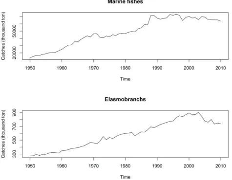
While the total worldwide marine fishes landings seem to have reached a plateau in the late 1980’s, elasmobranch catches increased progressively since the 1950’s until the early 2000’s, followed by a decreasing trend for the more recent years (Figure I.1). However, and even though the marine fish catches seem to have remained relatively stable since the late 1980’s, the fisheries have shifted in these last decades from catching mainly long lived high trophic level fishes, towards catching more short lived, low trophic level invertebrates and small planktivorous pelagic fishes (Pauly et al., 1998; Pauly and Palomares, 2005). This effect, originally called “fishing down the marine food web” by Pauly et al. (1998) shows that the marine ecosystems top predators (such as the sharks) are the first ones to suffer from overfishing and population declines. Indeed, most elasmobranchs are predators at, or near the top of the marine food webs (Cortés, 1999), and are extremely important for the entire ecosystems balance, by regulating not only their direct main preys, but also second and third degree non-prey species through the trophic linkages (Schindler et al., 2002). The effects of the removal of such predators from the marine ecosystems are difficult to foresee, but may be ecologically and economically significant, and may persist over long time periods (Stevens et al., 2000).
4
Figure I.1: Global capture of marine fishes (top) and elasmobranchs (bottom) from 1950 to 2010. Data from FAO FIGIS data collection (FAO, 2012)
Up until the 1980’s, elasmobranch fisheries were generally unimportant small fisheries, with generally a low commercial value. Traditionally, these elasmobranch fisheries of the past were multi-specific fisheries that caught several species of elasmobranchs depending on the region and season of the year. There was little interest in these fisheries, mainly due to their relatively small scale and low commercial value. Bonfil (1994) reported that cartilaginous fishes were a minor group which contributed with an average of 0.8% of the total world fishery landings between 1947 and 1985, while bony fishes such as clupeoids, gadoids and scombroids, accounted for 24.6%, 13.9% and 6.5%, respectively. In the last decades, however, the declining catches per unit effort (CPUE) and rising prices of traditional food fishes, along with the growing market for shark fins for the oriental markets, have made the previously underutilized elasmobranchs increasingly important resources (Castro et al., 1999).
The history of elasmobranch fisheries worldwide indicates, however, that these resources are usually not sustainable. Most elasmobranch targeted fisheries have been characterized by “boom and burst” scenarios, where an initial rapid increase of the exploitation and catches is followed by a rapid decline in catch rates and eventually a complete collapse of the fishery (Stevens et al., 2000). Bonfil (1994) and Shotton
5
(1999) provided reviews of world elasmobranch fisheries and included examples of situations where commercial catches have been declining, such as in the northeast Atlantic and Japan, and examples of situations of high concern such as in India. Baum et al. (2003) stated that the northwest populations of large pelagic sharks including the scalloped hammerhead, Sphyrna lewini, and the threshers Alopias vulpinus and A. superciliosus, have declined by more than 75% over the last 15 years, and even though the values presented in Baum et al. (2003) seem to have been severely overestimated (Burgess et al., 2005), there is consensus that there are currently causes for concern.
However, and even though overexploitation and population collapses is the most common scenario in elasmobranch fisheries, Walker (1998) demonstrated that elasmobranch stocks can be harvested sustainably and provide for stable fisheries when carefully managed. Some species such as the tope shark, Galeorhinus galeus, the sandbar shark, Carcharhinus plumbeus, the great white shark, Carcharodon carcharias and several species of dogfishes (order Squaliformes) have very low productivity and cannot withstand high levels of fishing, whereas other species such as the gummy shark, Mustelus antarcticus, the Atlantic sharpnose shark, Rhizoprionodon terraenovae, the bonnethead, Sphyrna tiburo and the blue shark, Prionace glauca have higher productivity and can support higher levels of fishing mortality (Walker, 1998).
Within the industrial oceanic fisheries such as longlines, driftnets and purse seines, the pelagic longlines are responsible for most of the captures of oceanic sharks at a global level, which are usually captured during the fishing operations that target swordfish and tunas (Aires-da-Silva et al., 2008). Several pelagic shark species are frequently caught in those oceanic longline fisheries, but the two most important and abundant are the blue shark, Prionace glauca, and the shortfin mako, Isurus oxyrhynchus. In the case of the Portuguese fishery, those two species together can account for more than 50% of the total oceanic longline fishery catch, and can represent more than 95% of the total elasmobranch catch (Coelho et al., 2012a).
I.3. The studied species, blue shark (Prionace glauca)
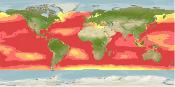
The blue shark (Prionace glauca) (Figure I.2) is one of the most wide ranging of all sharks, found throughout tropical and temperate seas from latitudes of about 60°N to
6
50°S (Last and Stevens, 2009) (Figure I.3). It is a pelagic species mainly distributed from the sea surface to depths of about 350 m, even though deeper dives of up to 1000m have been recorded (Campana, et al., 2011). The blue shark is an oceanic species capable of large scale migrations (Queiroz et al., 2005; Silva et al., 2010; Campana et al., 2011), but it can also occasionally occur closer to inshore waters, especially in areas where the continental shelf is narrow (Last and Stevens, 2009).
Figure I.2: The blue shark, Prionace glauca (Drawing by: João T. Tavares/Gobius).
Figure I.3: Global distribution map for the blue shark, Prionace glauca. The color scale represents the relative probabilities of occurrence, with red and yellow representing higher and lower probabilities of occurrence, respectively. Map generated from Fishbase (Froese and Pauly, 2012) using AquaMaps, a presence-only species distribution model (Ready et al., 2010).
The blue shark reaches a maximum size of about 380 cm total length (TL), and size at 50% maturity for the Atlantic has been estimated at 218 cm TL for males and
7
221 cm TL for females (Pratt, 1979). The blue shark is a placental viviparous shark, and shows a relatively high fecundity within the elasmobranchs, producing an average of 35 pups per litter (Zhu et al., 2011), with the maximum litter size recorded being 135 pups, after a gestation period of 9-12 months (Compagno, 1984; Castro and Mejuto, 1995; Snelson et al., 2008). The pups are born at 35-50 cm TL, and the reproductive cycle has been reported as seasonal in most areas, with the young being born usually in the spring and summer (Pratt, 1979; Stevens, 1984; Nakano, 1994; Hazin et al., 1994). Age and growth studies have suggested that longevity is of about 20 years, with the males maturing at 4-6 and females at 5-7 years of age (Stevens, 1975; Cailliet et al., 1983; Nakano, 1994; Skomal and Natanson, 2003; Lessa et al., 2004; Blanco-Parra et al., 2008; Megalofonou et al., 2009a). The diet of the blue shark consists mainly of small pelagic fishes and cephalopods, particularly squid (Vaske Jr. et al., 2009; Markaida and Sosa-Nishizaki, 2010; Preti et al., 2012). However, invertebrates such as pelagic crustaceans, small sharks, and seabirds have also been reported to be taken as food (Compagno, 1984).
Blue sharks are a highly migratory oceanic species, with complex movement patterns and spatial structure probably related to the reproduction cycles and prey distribution (Montealegre-Quijano and Vooren, 2010; Tavares et al., 2012). Some tagging studies have shown extensive movements of blue sharks in the Atlantic, with numerous trans-Atlantic migrations probably accomplished by using the major oceanic current systems (Stevens, 1976; Stevens 1990; Queiroz et al., 2005; Silva et al., 2010; Campana et al., 2011). At least in the north Atlantic, data on the distribution, movements and reproductive behavior seems to suggest a complex reproductive cycle, involving major oceanic migrations associated with mating areas in the north-western Atlantic and pupping areas in the north-eastern Atlantic (Pratt, 1979; Stevens, 1990).
The blue shark is possibly the most abundant of all pelagic shark species, and even though it can be captured by a variety of fishing gears, most captures take place as bycatch in pelagic longlines targeting tunas and swordfish (Aires-da-Silva et al., 2008; Stevens, 2009). In the Atlantic Ocean, the management of the oceanic tuna and tuna-like species (including pelagic sharks) is a mandate of ICCAT, the International Commission for the Conservation of Atlantic Tunas. ICCAT maintains the catch records from those fisheries (Figure I.4) and carries out stock assessments and other research initiatives for determining their vulnerability status.
8
Figure I.4: Nominal catches of all pelagic shark species by all oceanic fleets in the Atlantic Ocean (above), blue sharks captured by all fleets (center) and blue shark captured by the Portuguese fleet (below). Data from ICCAT Task1 (nominal catch information) database (ICCAT, 2012a).
Within the ICCAT scientific work, an Ecological Risk Assessment (ERA) was carried out for priority species of pelagic sharks in the Atlantic in 2010 (Cortés et al., 2010), with that analysis currently being updated with more recent information (Cortés et al., 2012). With both analyses it was demonstrated that most pelagic sharks have exceptionally limited biological productivity and, as such, can be overfished even at very low levels of fishing mortality, with the blue shark in particular shown to have an intermediate vulnerability. More recently, and for the Indian Ocean (managed by IOTC, the Indian Ocean Tuna Commission), an ERA analysis was also conducted for pelagic and some coastal shark species (Murua et al., 2012) and similar results were obtained for the blue shark, also characterized for having a relatively higher productivity but also a high susceptibility to longline fisheries, making it a species with an overall
9
intermediate level of vulnerability. The last blue shark stock assessment for the Atlantic Ocean was carried out by ICCAT in 2008 (ICCAT, 2009), and although a high level of uncertainty was reported in the models, the results showed that the current biomass was believed to be above the biomass that would support Maximum Sustainable Yield (MSY), and the harvest levels were believed to be below the Maximum Fishing Mortality (F) at MSY.
I.4. Challenges in modeling Chondrichthyans bycatch
The main goal of fisheries science and stock assessments are to inform decision makers on the potential consequences of different management actions, using the best available scientific information and data (Ludwig et al., 1993; Hilborn and Walters, 1992; McAllister et al., 1999; Quinn and Deriso 1999; Hilborn, 2006). The increasing concerns on the vulnerability of elasmobranch species to fisheries has lead, in recent years, to an increased interest on assessing the conservation status and carrying out stock assessments for those populations (McAllister et al., 2008). In general and when compared to other fishes, the current available information for assessing the status of elasmobranch populations is usually very poor, and as such most elasmobranchs are today in what is called data-poor situations. This is a situation characterized by little available information in terms of their biology (e.g. age and growth, reproduction, ecology, migratory movements), but also in terms of reliable time-series of their historical abundance and fisheries catches.
One commonly used analytical method that has been applied to some shark populations are demographic methods, which are useful particularly because they rely primarily on biological aspects (Cortés, 2002; Mollet and Cailliet, 2002), rather than on the historical catches or indexes of abundance. The inputs required are basic population dynamics parameters, such as the rate of survivorship at each age/stage, the duration of each life stage (in case of stage-based approaches), and the fecundity or number of newly born offspring produced per female at each age/stage. One important limitation on those methods is that they assume that there is no density-dependence, and that the estimated parameters are those of theoretical populations under stable conditions. Typical approaches for studying species demography include life table analysis (e.g.
10
Cailliet, 1992; Cortés, 1995) and matrix algebra analysis (e.g. Aires-da-Silva and Gallucci, 2007; Smith et al., 2008). The most important output of those methods for fisheries management is the estimation of r, the intrinsic rate of population increase under a stable condition and assuming density-independence, as this parameter provides an indication of the population resilience to exploitation.
For more elaborate and data-intensive stock assessment methods, one common approach used for some shark species are surplus production methods (e.g. shortfin mako assessment carried out by ICCAT, 2012b), that uses information from total catches and relative indexes of abundance of the stocks over time. Ideally, these indexes of abundance should be based on fishery-independent datasets, collected for example during scientific surveys using statistically adequate protocols (e.g. random sampling over predetermined strata such as area, season, year, etc). However, these type of data are very difficult to obtain and costly in the pelagic realm, as the sampling collection would have to occur in the high seas and cover very wide geographical areas. Therefore, and particularly when dealing with pelagic bycatch species such as sharks, the data available is usually based on fishery-dependent datasets, collected by commercial fishing vessels while operating during their normal fishing operations. Because of this, for calculating time series with the relative indexes of abundance useful for stock assessment, it is first necessary to adjust the data for the impacts of factors other than the changing abundances of the species over time. There are several methods for achieving this, but a recent common approach is to use statistical models such as Generalized Linear Models (GLM) to build the time series of the species abundance over time that only reflects the changes in the abundance, and where other effects inherent to the fishery-dependence itself have been removed. A good revision on the use of GLM for standardizing fishery-dependant datasets for stock assessment purposes was presented by Maunder and Punt (2004). For addressing the lack of independence in the data, alternative approaches such as Generalized Linear Mixed Models (GLMM) that use random effects on some variables allowing the introduction of variability (McCulloch and Searle, 2001; Bolker et al., 2009), and Generalized Estimating Equations (GEE) that introduce a dependence structure in the data (Zeger and Liang, 1986; Zeger et al., 1988), can be used.
Another potential issue and challenge when modeling data from shark populations is that the datasets of bycatch species often have some (sometimes many) fishing sets
11
with zero catches. Those represent the fishing sets that existed (have an associated effort), but resulted in zero catches for the species of concern, and this poses a special mathematical problem in terms of modeling. For example, one possible and common way of modeling catch rate data is to use GLM with a log link and some continuous distribution (e.g. Gaussian, Gamma), but in datasets with zeros adjustments need to be made for accommodating those observations, given that the log of zero is undefined. Possible solutions for those observations have ranged from simple solutions like adding a small constant to the observed data, to more complex approaches like zero-inflated models. Adding a small constant to the data was a common approach in the past, but as mentioned by Campbell (2004) the value of the constant to be added can be somewhat arbitrary and that constitutes a problem as bias are introduced in the analysis. Still, when the proportion of zeros in the datasets are low (<5-10% of the data), this approach is still commonly used in fisheries science. Besides this strategy, Maunder and Punt (2004) summarized other three classes of methods that can handle zero observations, specified as: 1) statistical distributions that allow for zero observations (e.g. Poisson, Negative Binomial, Tweedie); 2) methods that inflate the expected numbers of zeros (zero-inflated models); and 3) the delta-lognormal approach (Lo et al., 1992) that combines two separate models, usually one binomial model for modeling the proportion of positives and one continuous distribution model for modeling the predicted values conditional to the positive observations.
I.5. General objectives of the study with a note on the dissertation style
Given the general lack of information on the fisheries of the blue shark captured as bycatch in pelagic longline fisheries, and the increasingly importance of this species as a marine fisheries resource, there was a need to carry out a study focusing this species and its impacts in pelagic longline fisheries. The specific objectives of the present study were to:
1) Provide a general introduction to the Chondrichthyan fishes, their biology and susceptibility to fishing mortality, with a particular emphasis on the oceanic sharks and especially the blue shark (Chapter I);
12
2) Model the hooking mortality of the blue shark captured in the Portuguese longline fishery in the Atlantic Ocean (Chapter II);
3) Model the catch rates of the blue shark captured in the Portuguese longline fishery in the South Atlantic Ocean (Chapter III);
Each of the following chapters (specifically chapters II and III) of this thesis has been written in a paper-style format, suitable and appropriate to be published in a scientific journal. Each of those chapters constitutes a complete study and can be read independently of the others. At the beginning of each chapter information regarding that particular chapter publication status is given. Tables and figures appear in the text inside each chapter, but all acknowledgements have been compiled at the beginning of the thesis and all references have been compiled in a final section. A final Annex section is provided with a compilation of the R-language code that was produced and used in this thesis.
13
CHAPTER II. MODELING AT-HAULBACK MORTALITY OF BLUE SHARKS CAPTURED IN A PELAGIC LONGLINE FISHERY IN THE ATLANTIC OCEAN.1
II.1.Introduction
In the Atlantic Ocean several pelagic shark species are commonly bycatch on pelagic longline fisheries (e.g. Buencuerpo et al., 1998; Petersen et al., 2009; Simpfendorfer et al., 2002) but still, information on their life history, population parameters and the effects of fisheries on these populations is limited. Generally, elasmobranchs have K-strategy life cycles, characterized by slow growth rates and long lives, and reduced reproductive potential with few offspring and late maturity. The natural mortality rates are usually low, and increased fishing mortality may have severe consequences on these populations, with population declines occurring even at relatively low levels of fishing mortality (Smith et al., 1998; Stevens et al., 2000). Of the several elasmobranch species caught in surface pelagic longline fisheries, the blue shark, Prionace glauca, is the most frequently caught species (e.g. Coelho et al., 2012a).
Previous studies have focused on elasmobranch mortality during fishing operations, but most were carried out for coastal species caught in trawl fisheries. Those include the studies by Mandelman and Farrington (2007) for the spurdog (Squalus acanthias) and Rodríguez-Cabello et al. (2005) for the small-spotted catshark (Scyliorhinus canicula). For pelagic elasmobranchs caught in pelagic fisheries in the NW Atlantic Ocean, Campana et al. (2009) analyzed blue sharks captured by the Canadian fleet and studied both the short term mortality (recorded at-haulback) and the longer term mortality (recorded with satellite telemetry). Also for the NW Atlantic, Diaz and Serafy (2005) worked with data from the U.S. pelagic fishery observer program and analyzed factors affecting the live release of blue sharks.
Knowledge on the at-haulback mortality can be used to evaluate conservation and management measures that include the prohibition to retain particular vulnerable
1
Based on a published manuscript: Coelho, R., Infante, P. & Santos, M.N. 2013. Application of Generalized Linear Models and Generalized Estimation Equations to model at-haulback mortality of blue sharks captured in a pelagic longline fishery in the Atlantic Ocean. Fisheries Research, 145: 66-75.
14
species, such as those recently implemented by some tuna Regional Fisheries Management Organizations (tRFMOs). In particular and for the Atlantic Ocean, the International Commission for the Conservation of Atlantic Tunas (ICCAT) has recently implemented mandatory discards for the bigeye thresher (ICCAT Rec. 09-07), the oceanic whitetip (ICCAT Rec. 10-07), hammerheads (ICCAT Rec. 10-08) and silky sharks (ICCAT Rec. 11-08). However, important parameters, such as the at-haulback fishing mortality (recorded at time of fishing gear retrieval), remain largely unknown and therefore the efficiency of such measures also remains unknown. Even considering that all specimens of these particular species are now being discarded, fishing mortality is still occurring due to at-haulback mortality, as part of the catch is already dead at time of fishing gear retrieval and is therefore being discarded dead.
At-haulback mortality studies are also important as they can be incorporated into stock assessments, such as the study by Cortés et al. (2010), which used an ecological risk assessment analysis for eleven species of elasmobranchs captured in pelagic longlines in the Atlantic Ocean. With this analysis, both the susceptibility and the productivity of each species are analyzed in order to rank and compare their vulnerability to the fishery. One of the parameters that can be included in the susceptibility component is the probability of survival after capture, which can in part be inferred from the mortality at-haulback.
This study had two main objectives:
1) to compare the use of Generalized Linear Models (GLM) and Generalized Estimation Equations (GEE) for predicting the at-haulback mortality of blue sharks captured in the Portuguese pelagic longline fishery in the Atlantic Ocean targeting swordfish and,
2) to identify variables that are significant and influence the blue shark at-haulback mortality rates.
15
II.2.Material and Methods II.2.1. Data collection
Data for this study was collected by fishery observers from the Portuguese Institute for Sea and Atmospheric Research (IPMA, I.P.) that were placed onboard Portuguese longliners targeting swordfish along the Atlantic Ocean. Data was collected between August 2008 and December 2011. During that period, information from a total of 762 longline sets corresponding to 1,005,486 hooks was collected. The study covered a wide geographical area (from both hemispheres) of the Atlantic Ocean (Figure II.1).
Figure II.1: Location of the longline fishing sets analyzed in this study along the Atlantic Ocean. The scale bar is represented in nautical miles (NM).
For every specimen that was caught, onboard fishery observers recorded the species, specimen size (FL, fork length measured to the nearest lower cm), sex, at-haulback condition (alive or dead at time of fishing gear retrieval), fate (retained or discarded), and the condition if discarded (alive or dead at time of discarding). For each
16
longline set carried out some additional information was recorded, including date, geographic location (coordinates: latitude and longitude), number of hooks deployed in the set, and branch line material used (monofilament or wire). Additional variables relative to the fishing sets that were calculated a posteriori included the Sea Surface Temperature (SST), which was interpolated from satellite data using the known date and location of each fishing set. The algorithm used to interpolate SST data followed the methods described by Kilpatrick et al. (2001), and was applied using the Marine Geospatial Ecology Tools (MGET) developed by Roberts et al. (2010).
II.2.2. Preliminary data analysis
The length frequency distribution of male and female blue sharks captured was analyzed, and compared with a 2-sample Kolmogorov–Smirnov test and a Mann Whitney rank sum test. Those non-parametric tests were chosen after calculating the skewness and kurtosis coefficients for the data, and confirming that the data was non-normal with a Lilliefors test. The proportions of dead and alive blue sharks were calculated for each level of each categorical covariate (trip, sex, year, quarter, vessel, branch line material), and the differences in the proportions were compared with contingency tables and Chi-square statistics (using Yates’ continuity correction in the cases of 2x2 tables). For this preliminary analysis, the continuous variables FL, latitude, longitude and SST were categorized by their quartiles.
II.2.3. Statistical Modeling
Generalized Linear Models (GLM) and Generalized Estimation Equations (GEE) were used to model blue shark at-haulback mortality, and compare the odds of a shark being dead at-haulback given the various variables considered. The response variable was the condition of the specimens at time of haulback (Yi: binominal variable, i.e., dead or alive), and for this study we considered that the event occurred if the shark died during the fishing operation. Therefore, the response variable was coded with 1 for sharks dead at-haulback and coded with 0 for sharks alive at-haulback.
17
Each captured shark (Yi) follows a Bernoulli distribution with pi (probability of success versus dying at-haulback = πi), and can be specified as:
~ (1, )
With the expected value and the variance defined by: ( ) =
( ) = × (1 − )
The relationship (link function) between the mean value of Yi and the model covariates considered for this model was the logit, and the model was therefore defined by:
( ) = 1 − = + , + , + ⋯ + ,
Where xi are the model variables and β are the coefficients that were estimated by maximum likelihood.
The explanatory variables initially considered for the model were the specimen size (FL in cm), sex (male or female), fishing location (latitude and longitude in decimal degrees), year (2008 to 2011), quarter of the year (1 = January to March, 2 = April to June, 3 = July to September and 4 = October to December), vessel identity (two vessels involved in the study), branch line material (wire or monofilament) and SST (decimal degrees in ºC). Some potential additional variables were not considered due to being unbalanced or correlated with other variables, such as the month with quarter of the year, and fishing trip with vessel.
The first modeling approach was carried out with GLM. The univariate significance of each explanatory variable was determined by the Wald statistic and with likelihood ratio tests, comparing each univariate model with the null model. The significant variables were then used to construct a simple effect multivariate GLM, with the non-significant variables (at the 5% level) eliminated consecutively from the model. The significance of each variable was determined by the Wald statistic and by an analysis of deviance table. At this stage, the variables had been eliminated in the first step were further tested, in order to determine an eventual significance within the
18
framework of a multivariate model, as recommended by Hosmer and Lemeshow (2000). Once a final multivariate simple effects model using only significant variables was obtained, each pair of possible first degree interactions between variables was tested. The interactions were considered for inclusion in the final model if significant at the 1% level both with the Wald statistic, and with likelihood ratio tests comparing the models with and without the interaction.
The GLM assumptions in terms of both the continuous and categorical explanatory variables were assessed. Regarding the continuous variables, GLM have the assumption that those variables are linear with the linear predictor (in this case the logit) and such linearity was assessed with the method of discretizing the continuous variables by the quartiles as described by Hosmer and Lemeshow (2000), and by analyzing GAM plots. If transformations were required, then the best possible solution was estimated with multivariate fractional polynomials and the transformed variables were used in the models instead of the original values, following the method developed by Royston and Altman (1994) and recommended by Hosmer and Lemeshow (2000). Regarding the categorical variables, GLM assume that all levels of the categories have sufficient information in the binomial response to allow contrasts in the data and achieve model convergence. These assumptions follow the contingency tables and Chi-square tests assumptions, in which the contingency tables should not have cells with zero values, or more than 25% of the cells with predicted values lower than 5. These assumptions were validated by building contingency tables for all categorical variables that were considered.
Another assumption in the GLM modeling approach is that the data in the sample should be independent, in this case that the Yi correspond to a succession of independent Bernoulli trials. Given that the data used in this study is fisheries-dependant data, it is plausible to consider that this assumption was not validated. Therefore an alternative modeling approach with Generalized Estimation Equations (GEE) was considered as this allows for a working correlation to be estimated within the data. Within this GEE model framework, the fishing set was considered as the grouping variable, meaning that the data could be considered to be clustered and not independent within each fishing set. This allowed for a model formulation in which the blue shark at-haulback mortality data recorded within each fishing set carried out by each particular vessel in each particular fishing trip did not require the assumption of independence. With this GEE model
19
formulation, the correlation structure of the data within each set was assumed to be of the type exchangeable, as this seems to be the most adequate correlation structure for clustered data (Halekoh et al., 2006).
With the final model estimated, examples of model interpretation were presented. One parameters that is important to interpret in biological terms in the specimen size, and therefore the probabilities of a shark dying at-haulback with varying specimen sizes were calculated. Additionally, the odds-ratios for increasing specimen sizes by 10cm FL (also calculated along the range of shark sizes in the sample), were also calculated and presented. The probabilities were calculated as the inverse-logit function of the final equations considered, and the odds-ratios were calculated as the exponential values of the differences (in 10cm FL sizes) in the logits. For this specific example, the variables that were interacting with FL were considered to be on their baseline levels.
II.2.4. Diagnostics and goodness-of-fit
A residual analysis using Pearson and Deviance residuals was used to search for outliers, and the Cooks distances and DfBetas were used to identify eventual values with influence in the estimated parameters of the models. Model goodness-of-fit was assessed with the Hosmer and Lemeshow statistic that groups the observations into 10% quantiles (deciles) according to their predicted values, and uses a chi-square test for comparing the observed versus predicted values in each group (Hosmer and Lemeshow, 2000). Additionally, the Nagelkerke coefficient of determination (R2) (Nagelkerke, 1991) was also calculated. The discriminative capacity of the models was determined by the Area Under the Curve (AUC) value of the Receiver Operating Characteristic (ROC) curves, with the determinations of the model sensitivity (capacity to correctly detect the event = mortality at-haulback) and model specificity (capacity to correctly exclude sharks not dead at-haulback).
Cross validation was carried out with a k-fold cross validation procedure (with k=10) to estimate the expected level of fit of the models to new data, and to assess eventual over-fitting problems. Because the models in this study are of the binomial type, the cross validation procedure was used to estimate the misclassification error rate, with the procedure randomly partitioning the original sample into k-subsamples, and
20
then retaining one subsample as the validation dataset and using the remaining k-1 subsamples as training datasets to build the models. The cross-validation procedure was repeated k times, with each of the k subsamples used one time as the validation dataset, and the use of k=10 was chosen as this seems to be an adequate value for models using large datasets (Fushiki, 2011). Finally, a bootstrapped cross validation procedure was also used to calculate new AUC values, that were compared to the original AUC calculated using the entire dataset.
All statistical analysis for this study was carried out with the R Project for Statistical Computing version 2.14.1 (R Development Core Team, 2012). Most functions are available in the core R Program, but some analysis required additional libraries, including library “gmodels” (Warnes, 2011a) for the contingency table analysis, library “gplots” (Warnes, 2011b) for some of the graphics produced, library “moments” (Komsta and Novomestky, 2012) for data summaries including the kurtosis and skewness coefficients, library “gam” (Hastie, 2011) for the GAM models and plots, library “mfp” (Ambler & Benner, 2010) for the multivariate fractional polynomials transformations, library “geepack” (Halekoh et al., 2006) for the GEE models, library “Epi” (Carstensen et al., 2011) for the ROC curve plots, and library “boot” (Canty and Ripley, 2011) for the cross validation procedure.
II.3.Results
II.3.1. Description of the catches
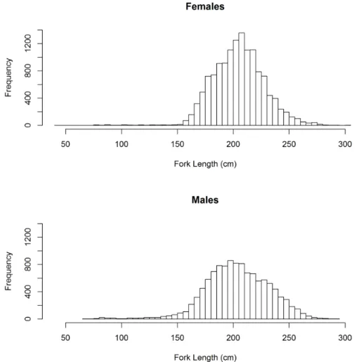
A total of 26,383 blue shark specimens were captured and recorded during the sampling period. Of those, complete capture information including at-haulback condition, size, sex, date and coordinates of the capture was available for 24,958 specimens (94.6% of the blue shark catch) and the analysis was therefore performed on those specimens. Of the specimens analyzed, 13,530 (54.2%) were females, while the remaining 11,428 (45.8%) were males. The females mean size in the sample was 199.5 cm FL (SD = 31.7) with the distribution ranging from 40 to 305 cm FL, while the males had a mean size of 194.5 (SD= 36.9) and the size distribution ranged from 69 to 295 cm FL (Figure II.2). The size distribution of males and females was considered significantly different, given that the null hypothesis that both sexes come from the
21
same continuous distribution was rejected (2-sample Kolmogorov-Smirnov test: D = 0.06, p-value < 0.001). Likewise, the ranks of the sizes of males and females was also significantly different (Mann-Whitney test: W = 7.9e+7, p-value = 0.002). The non-normality in the size data was confirmed with a Lilliefors test (D = 0.030, p-value < 0.001), with the data having a skewness coefficient of -0.41 (negatively asymmetrical) and a kurtosis coefficient of 4.99 (leptokurtic data). Note that the kurtosis coefficient used was calculated as the ratio between the 4th sample moment and the square of 2nd sample moment, and therefore the reference value for a mesokurtic sample would have been 3.
Figure II.2: Size frequency distribution of female and male blue sharks captured and analyzed during this study.
22
II.3.2. Proportions of hooking mortality
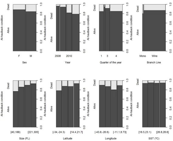
In general terms, 13.3% of the blue shark specimens that were captured during this study were dead at-haulback, while the remaining 86.7% were alive. In terms of the categorical variables, the proportions of alive:dead blue sharks were significantly different between all levels of the variables that were initially considered, specifically fishing trip (chi-square = 2092.5, df = 13, p-value < 0.001), sexes (chi-square = 94.4, df = 1, p-value < 0.001), year square = 1191.2, df = 3, p-value < 0.001), quarter (chi-square = 193.8, df = 3, value < 0.001), vessel identity (chi-(chi-square = 181.3, df = 1, p-value < 0.001) and branch line material (chi-square = 39.4, df = 1, p-p-value < 0.001) (Figure II.3).
Regarding the continuous variables, and considering the data grouped by the quartiles, the proportions of alive:dead sharks were different between sizes (chi-square = 833.5, df = 3, p-value < 0.001), latitude (chi-square = 643.2, df = 3, p-value < 0.001) and longitude (chi-square = 323.3, df = 3, p-value < 0.001), but not significantly different considering SST (chi-square = 2.8, df = 3, p-value = 0.419) (Figure II.3). Besides not being significant in the contingency table analysis, the SST was also found to be significantly correlated with latitude (Pearson correlation = 0.605, p-value < 0.001; Spearman correlation = 0.581, p-value < 0.001), and with longitude (Pearson correlation = -0.363, p-value = 0.001; Spearman correlation = -0.353, p-value < 0.001) which might create multicollinearity problems if both the SST and the geographical coordinates were used as explanatory variables in a multivariate model. Additionally, and because the geographical coordinates were available for all fishing sets, while SST was only available for part of the sets (specifically for 231 of the 762 sets carried out), the SST variable was discarded and not used in the final models.
23
Figure II.3: Proportions of alive and dead blue sharks at-haulback with the various categorical and continuous explanatory variables considered for the analysis. The continuous variables are categorized by their quartiles.
II.3.3. Simple effects GLM and GEE models
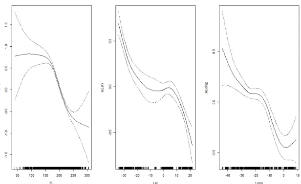
The functional form of the continuous explanatory variables (FL, latitude and longitude) was assessed with GAM plots. The at-haulback mortality tended to decrease with increasing specimen size, towards northern latitudes and eastern longitudes (Figure II.4).
24
Figure II.4. Generalized Additive Model (GAM) plots with the shape of the continuous explanatory variables (FL, latitude and longitude) for modeling blue shark at-haulback mortality.
As verified with multivariate fractional polynomials models, only the longitude was significantly linear, while the specimen size and latitude were non-linear variables that needed to be transformed in order to be used within the assumptions of GLM. By applying the multivariate fractional polynomial transformations to those three continuous variables, the best candidate alternatives to the transformations of the functional form were:
Size (FL): !"#$ .&+ !"#
Latitude: "'()*+. # + "'()*+. #* Longitude: ",-.)+*./#
The transformation regarding the longitude is a simple scale transformation, while the transformations for specimen size and latitude refer to transformations in the functional form. These transformed variables were used in the models instead of the original values.
25
In the simple effects multivariate model, all the variables that were initially considered were significant at the 5% level except the vessel effect. Regarding the quarter of the year the overall effect was significant, but no differences were found between quarters 1 and 2 (Wald statistic: z = -0.323; p-value = 0.747) and quarters 1 and 4 (Wald statistic: z = 0.578; p-value = 0.563). Therefore, this variable was simplified into a binomial variable (season), coded with: season 1 = quarter 3 and season 2 = quarters 1, 2 and 4.
The results of the simple effects GLM parameters in terms of significance are given in the analysis of deviance presented in Table II.1, where it is possible to see the contribution of each parameter for explaining part of the deviance observed in the blue shark at-haulback mortality. The parameters that are contributing more for the model deviance explanation are the effects of the year and specimen size, followed by the geographical location of the capture (latitude and longitude). Finally, the effects of season, branch line material and sex are contributing less for the blue shark at-haulback mortality deviance explanation, but are still significant variables in the model (Table II.1).
Table II.1. Deviance table for the simple effects GLM for the binomial response (alive or dead) status of blue sharks at-haulback. Resid.df are the residual degrees of freedom and Resid.dev is the residual deviance. Significance of the terms is given by the p-values of the chi-square test. The “.t” notations after the continuous variables (FL, Lat and Long) represent the utilization of the transformed variables in the models.
Parameter Df Deviance Resid.df Resid.dev p-value
Null 24957 19561 FL.t 1 645.24 24956 18915 < 0.001 Latitude.t 1 273.10 24955 18642 < 0.001 Longitude.t 1 251.79 24954 18390 < 0.001 Year 3 908.63 24951 17482 < 0.001 Season 1 11.06 24950 17471 < 0.001 Branch line 1 7.07 24949 17464 0.008 Sex 1 12.71 24948 17451 < 0.001
When applying a GEE model to those variables, and considering the fishing set as the grouping (cluster) variable, the estimated correlation value was low (alpha = 0.058, SE = 0.019), and the estimated parameters were very similar between the GLM and
26
GEE models, with only some minor differences (Table II.2). The overall parameter interpretation would be similar with both modeling approaches, given that the parameters were consistently positive or negative when comparing the models. The only major different in these multivariate simple effects models was that the effect of sex was significant in the GLM model but not significant (at the 5% level) within the GEE framework (Table II.2).
Table II.2. Multivariate simple effect GLM and GEE model parameters (coefficients and standard errors) for the binomial response (alive or dead) status of blue sharks at haulback. Significance of the explanatory variables is given by the Wald statistic with the respective p-values. The “.t” notations after the continuous variables (FL, Lat and Long) represent the utilization of the transformed variables in the models.
Variable Generalized Linear Model Generalized Estimating Eq. Estimate SE Wald p-value Estimate SE Wald p-value
Intercept 3.95 0.35 11.4 < 0.001 4.29 0.49 75.9 < 0.001 FL.t -4.19 0.23 -18.5 < 0.001 -4.29 0.34 156.4 < 0.001 Lat.t -0.01 0.00 -14.5 < 0.001 -0.01 0.01 60.0 < 0.001 Long.t -0.25 0.02 -10.4 < 0.001 -0.21 0.05 19.5 < 0.001 Year2009 0.51 0.11 4.7 < 0.001 0.41 0.18 5.3 0.021 Year2010 1.60 0.09 16.8 < 0.001 1.34 0.18 58.6 < 0.001 Year2011 1.79 0.09 19.5 < 0.001 1.70 0.16 114.3 < 0.001 Season2 -0.19 0.07 -3.0 0.003 -0.23 0.10 5.2 0.023 BranchWire -0.19 0.09 -2.3 0.022 -0.28 0.12 5.6 0.018 SexMale 0.15 0.04 3.6 < 0.001 0.06 0.05 1.7 0.197
II.3.4. Models with interactions
Several possible 1st degree interactions between the variables were significant at the 1% significance level and therefore a model with significant interactions was created. In this model, year and specimen size were still the most important explanatory variables, followed by the location, season, branch line material and sex (Table II.3). In terms of interactions, specimen size was significantly interacting with longitude and year; specimen sex was interacting with longitude and season; longitude was interacting with season; and branch line material was interacting with year (Table II.3). The interactions between longitude and season, and between year and branch line material seemed to be particular significant in this model, with relatively high values of deviance (Table II.3).
27
Table II.3. Deviance table for the GLM model with significant 1st degree interactions for the binomial response (alive or dead) status of blue sharks at-haulback. Resid.df are the residual degrees of freedom and Resid.dev is the residual deviance. Significance of the terms is given by the p-values. The “.t” notations after the continuous variables (FL, Lat and Long) represents the use of transformed variables in the models.
Parameter Df Deviance Resid.df Resid.dev p-value
Null 24957 19561 FL.t 1 645.24 24956 18915 < 0.001 Lat.t 1 273.1 24955 18642 < 0.001 Long.t 1 251.79 24954 18390 < 0.001 Year 3 908.63 24951 17482 < 0.001 Season 1 11.06 24950 17471 0.001 Branch line 1 7.07 24949 17464 0.008 Sex 1 12.71 24948 17451 < 0.001 FL.t:Long.t 1 13.62 24947 17437 < 0.001 FL.t:Year 3 41.96 24944 17395 < 0.001 Long.t:Season 1 71.25 24943 17324 < 0.001 Long.t:Sex 1 15.06 24942 17309 < 0.001 Year:Branchline 3 80.81 24939 17228 < 0.001 Season:Sex 1 8.71 24938 17220 0.003
Like with the simple effects model, a GEE model was also applied to this case (considering interactions), again considering the fishing set as the grouping (cluster) variable. Like in the simple effects model, the correlation within the fishing set was low (alpha = 0.051, SE = 0.022), and the parameters estimated with both the GLM and GEE models were similar, with consistently positive or negative parameters (Table II.4). In this case, the only major difference between using GLM or GEE was the loss of significance (at the 1% significance level) for the interaction between season and specimen sex (Table II.4).
28
Table II.4. Multivariate GLM and GEE parameters of the models with significant 1st degree interactions (coefficients and standard errors) for the binomial response (alive or dead) status of blue sharks at-haulback. Significance of the explanatory variables is given by the Wald statistic with the respective p-values. The “.t” after the continuous variables (FL, Lat and Long) represents the use of transformed variables in the models.
Variable Generalized Linear Model Generalized Estimating Eq. Estimate SE Wald p-value Estimate SE Wald p-value
Intercept 3.90 1.26 3.1 0.002 2.50 1.39 3.2 0.073 FL.t -4.24 0.88 -4.8 < 0.001 -3.21 0.98 10.8 0.001 Lat.t -0.01 0.00 -13.4 < 0.001 -0.01 0.00 52.8 < 0.001 Long.t -0.96 0.29 -3.3 0.001 -0.50 0.42 1.4 0.231 Year2009 7.85 1.67 4.7 < 0.001 6.49 1.90 11.6 0.001 Year2010 2.32 1.34 1.7 0.083 2.61 1.58 2.7 0.100 Year2011 5.70 1.35 4.2 < 0.001 5.52 1.44 14.6 < 0.001 Season2 0.85 0.18 4.7 < 0.001 0.78 0.27 8.3 0.004 BranchWire -1.26 0.21 -6.0 < 0.001 -1.25 0.27 22.3 < 0.001 SexMale 0.17 0.17 1.0 0.301 0.30 0.16 3.6 0.056 FL.t:Long.t 0.83 0.20 4.1 < 0.001 0.51 0.30 2.9 0.087 FL.t:Year2009 -5.47 1.19 -4.6 < 0.001 -4.51 1.37 10.8 0.001 FL.t:Year2010 -1.85 0.94 -2.0 0.050 -2.07 1.10 3.5 0.060 FL.t:Year2011 -3.61 0.96 -3.8 < 0.001 -3.52 1.03 11.8 0.001 Long.t:Season2 -0.49 0.05 -9.0 < 0.001 -0.44 0.09 21.9 < 0.001 Long.t:SexMale -0.12 0.04 -3.0 0.003 -0.13 0.04 12.1 0.001 Year2009: BranchWire 0.04 0.29 0.1 0.894 0.01 0.37 0.0 0.983 Year2010: BranchWire 2.12 0.30 7.0 < 0.001 1.94 0.42 21.3 < 0.001 Year2011: BranchWire 1.42 0.24 6.0 < 0.001 1.41 0.30 22.1 < 0.001 Season2:SexMale 0.36 0.12 3.0 0.003 0.14 0.12 1.5 0.226
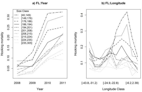
By using significant interactions, model interpretation gets more complex as the effects of the interacting variables need to be considered at the same time. Regarding the interaction between size and year, the at-haulback mortality for all size classes tended to increase along the years, but the relative increase was different between sizes, with the smaller specimens having a more sharp increase in mortality for the more recent years (Figure II.5). In terms of the relation between size and longitude, the at-haulback mortality remained at relatively low levels for the larger size classes throughout the entire longitude range, while a peak of at-haulback mortality was observed for the smaller size classes towards the eastern longitudes (Figure II.5).
29
Figure II.5. Interactions between specimen size (FL) with year (a) and longitude (b). The classes of the continuous variables specimen size and longitude are categorized by the deciles.
The categorical variable sex was significantly interacting with both season and longitude (Figure II.6). On both cases the male mortality rates tended to be higher than that for females, but there were some small differences in the changing patterns. For the relation between sex and season there was an increased mortality during the combined winter (autumn to spring) season, but the increasing rate was higher for males than for females (Figure II.6).
The other significant 1st degree interaction considered in the model was between branch line material and year. In general terms, the at-haulback mortality when using monofilament branch lines remained relatively high between 2008 and 2011 (except for 2010, when a decrease was observed), while an increasing trend along the time period was observed for wire branch lines (Figure II.6).
30
Figure II.6. Interactions plots between specimen sex with season (a), sex with longitude (b), season with longitude (c) and branch line material with year (d). The classes of the continuous variable longitude are categorized by the deciles.
II.3.5. Diagnostics and goodness-of-fit
For the final multivariate model, validation with the Pearson and Deviance residuals confirmed that there were no values that presented major and significant outliers (Figure II.7). For the Cooks distances two points presented values relatively higher than the remaining and those could possibly be values with influence in the estimated parameters (Figure II.7).
31
Figure II.7: Residual analysis (Pearson and Deviance residuals) and leverage values (Cooks distances) for the final GLM model including the main effects and the 1st degree interactions. The residuals are plotted in terms of the predicted values and the Cooks distances along the data index. A half-normal plot of the Cooks distances is presented to help identify the extreme values.
The DfBetas were also calculated, identifying possible observations that had more influence in the parameter estimation. Two observations seem to be possibly influential (Figure II.8), with those two observations corresponding to the values that had also been identified with the Cooks distances, specifically the data points 17,469 and 17,487 in the dataset used for the models.
Because of those two observations, two new models were created, with each new model excluding each of those data points identified. The results of the new models with the respective new estimated parameters and SE are presented in Table II.5. It is possible to see that for most of the parameters the differences in the estimations are
32
relatively small and lower than 20%. In terms of improvement of the explained deviance, by removing these possible influential values the differences were almost negligible, with the improvement in the R2 of the two alternative models lower than 0.2% when compared to the original model using all data points. Because the differences in the estimated parameters were in general small, and the improvements in terms of the deviance explained are almost negligible, the remaining model diagnostics, goodness-of-fit and model discriminative capacity were tested for the original models using all data points in the dataset and without excluding any possible outliers or influential values.
Figure II.8. Df Betas for the final GLM model including the main effects and interactions. The DfBetas are plotted along the predicted values, and the two observations that are possibly influential in some of the estimated parameters are identified.