A local grid refinement technique based upon Richardson extrapolation

(1)

upon Richardson extrapolation

P.

J.

Coeiho

Instituto Superior Tkcnico, Technical University of Lisbon, Mechanical Engineering Department, Lisboa, Portugal

J. Argain

University of Algarue, Physics Department, Faro, Portugal

A grid-embedding technique for the solution of two-dimensional incompressible flows gouemed by the Nauier-Stokes equations is presented. A single coarse grid covers the whole domain, and local grid refinement is carried out in the resions of high gradients without changing the basic grid structure. A finite volume method with collocated primitive variables is employed, ensuring conservation at the interfaces of embedded grids, as well as global conservation. The method is applied to the simulation of a turbulent flow past a backward facing step, the flow over a square obstacle, and the flow in a sudden pipe expansion, and the predictions are compared with data published in the literature. They show that neither the convergence rate nor the stability of the method are affected by the presence of embedded grids. The grid-embedding technique yields significant savings in computing time to achieve the same accuracy obtained using conventional grids. 0 1997 by Elsevier Science Inc.

Keywords: local grid refinement, grid embedding, Richardson extrapolation

1. Introduction

The numerical solution of fluid flow problems governed by the Navier-Stokes equations is generally accomplished using finite volume, finite difference, or finite element methods. The physical domain is mapped using a grid that should be more refined in regions of high gradients of the dependent variables or their derivatives. If a structured grid is used, extended over the whole domain, it often happens that many grid nodes are placed in regions of smooth change of the dependent variables. In such a case there is a high computational penalty, which could be avoided by using a domain decomposition approach. Sev- eral techniques of this kind have been developed, such as overlapping grids,’ zonal methods,’ and grid-embedding techniques.3

In grid-embedding or local grid refinement techniques a single coarse grid covers the whole domain and local

Address reprint requests to Dr. Coelho at the Instituto Superior Te’cnico, Departamento de Engenharia Mecanica, Av. Rovisco Pais, 1096 Lisboa codex, Portugal.

Received 18 April 1997.

Appl. Math. Modelling 1997, 21:427-436, July 0 1997 by Elsevier Science Inc.

655 Avenue of the Americas, New York, NY 10010

refinement is carried out in the regions of high gradients without changing the basic grid structure. These techniques often have been applied to the prediction of com- pressible flows using the full potential equation4 the Euler equation3 or the Navier-Stokes equations.’ Adap- tive local grid refinement has been used in the solution of the Euler,6T7 and Navier-Stokes equations,‘T9 including a parallel Navier-Stokes algorithm.” Multigrid has also been coupled with grid embedding.“*‘* However the use of grid-embedding techniques in the solution of incompressible flows using pressure-correction algorithms has received much less attention. They have been used to calculate laminar flow~,‘~,‘~ but either the details are not providedi or conservation of the fluxes along the interfaces is not ensured.14 Local grid refinement has also been employed in the framework of multigrid techniques to calculate incompressible flows, where the finest grids do not extend over the whole domain.‘5-‘7

A new grid-embedding technique was reported by Coelho et a1.18 and applied to the calculation of incompressible laminar recirculating flows. It solves the Navier-Stokes equations using primitive variables and a nonstaggered grid variable arrangement. A finite volume/finite difference method is used to discretize the

0307-904X/97/$17.00 PII s0307-904x(97)00037-1

(2)

equations, and the treatment of the interfaces is fully conservative. The whole domain is treated simultaneously regardless of the level of grid refinement. This enhances the coupling between regions of different levels of refinement and does not reduce either the convergence rate or the stability of the method. This contrasts with some other methods where the regions with different refinement levels are treated sequentially, and the only interaction among the different subdomains is done by transferring boundary data. The method was also applied to the calculation of laminar diffusion flames.” However, owing to the treatment of the interfaces between regions of different refinement levels, the extension of the method described in Coelho et all8 to turbulent flows was cumbersome. A modification of that treatment is presented in this paper, which enables a straightforward extension to turbulent flows.

The method is applied to the calculation of several turbulent recirculating flows, including the flow past a backward-facing step, the flow over a square obstacle, and the flow in a sudden pipe expansion. A description of the method is given in the next section. Then the results are presented and discussed, and the paper ends with a sum- mary of the main conclusions.

Using this data structure, and provided that the refinement ratio is kept equal to two, all possible interfaces are of the kind depicted in Figures 1 and 2, irrespective of the refinement level. No additional complications arise from the use of several levels of grid refinement. It is only necessary to give as input the refinement level desired for each cell of the coarsest grid. Further details of the data structure are given elsewhere.”

2.2

Discretization procedure

The time-averaged differential equations describing conservation of mass and momentum for a steady high Reynolds number flow, closed using the standard k-E turbulence model, may be written as follows:

(2)

2. The numerical procedure

2.1 Grid and data structure

The physical domain is discretized using a rectangular coarse mesh, which is locally refined in regions of high gradients. Local grid refinement is performed by halving on a cell-by-cell basis the mesh spacing in both X- and y-directions. This process may be repeated, leading to an

arbitrary number of refinement levels.

Each control volume is numbered sequentially and its north, south, east, and west neighbors are stored in one- dimensional arrays. The dimension of these arrays is slightly larger than the total number of grid nodes. This small overhead in the dimension of the arrays is required to keep track of the interfaces between regions of different grid refinement. Three additional points are stored for each interface between regions of different refinement level: two on the coarser side of the interface and one on the opposite side. These auxiliary points are also stored sequentially.

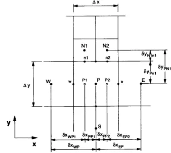
Figure 1

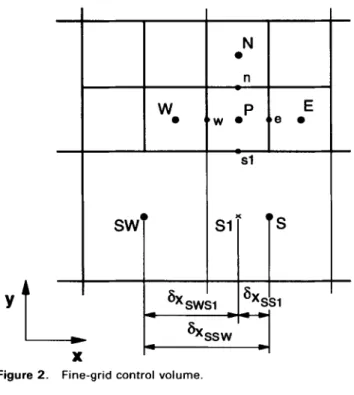
shows a typical control volume centered at node P with two neighbors on the northern face, Nl and N2. The south neighbor of grid node Nl is an auxiliary point denoted as Pl, and the south neighbor of grid node N2 is the auxiliary point P2. These auxiliary points P, and P, have west and east neighbors (grid nodes W and P for point Pl, and grid nodes P and E for point P,, respectively). This connectivity is stored in memory, as mentioned above. Figure 2 shows a control volume centered at P, which has an auxiliary point, denoted by Sl, as its south neighbor. The west and east neighbors of the auxiliary point Sl are the grid nodes SW and S, respectively.

a

I-%

a&

i

I

E2

=-

--

dxj

U,

axj

-

c,;p+Tjz

_J

-c,

pk

(4)

In these equations ui is the mean velocity component along direction xi,

p

is the pressure,

p

is the density, k is the turbulent kinetic energy, and E is the dissipation rate.

I I I Nl N2 . . Ill n2 6YbA”l ’ “EP _ _

(3)

- - I -

T

w

l

SW

i

N

I

0 n P E W. e l

A_

sl

Y

f

I

Figure 2. Fine-grid control volume.

The Reynolds stresses are determined as

-

(5)

where sij is the kronecker symbol and pI = C, pk2/& is the turbulent viscosity. Standard values2’ are assigned to the constants of the model CC,, C,, a,, Us, C,>. This model is not valid close to the walls, where low Reynolds numbers occur. The laws of the wa112’ are used in the boundary conditions to treat the near-wall region.

The governing equations are discretized using a finite volume/finite difference method. If mesh embedding is not considered, the governing discretized equations can be cast in the following form2’:

aA=

Cai4i+b

(6)

where the index i runs over all neighboring points (N, S, E, and W), b denotes the source term, and the coefficients ap and ai are combined convection/diffusion fluxes across the faces of the control volume. They are computed using the hybrid central differences/upwipd scheme for the discretization of the convective terms, and central differences for the diffusive terms.

When grid embedding is used, interfaces between regions of different refinement need particular attention. In all such interfaces there is one grid node on one side of the interface and two grid nodes on the other side, as sketched in Figure 1. To exemplify the method developed here, the north face of the P control volume shown in that figuri is considered

handled similarly. Special care was across the interfaces.

below. Other interfaces would be taken to ensure flux conservation This is automatically ensured if the

fluxes are calculated in the same way for grid nodes on both sides of the interface. Hence the fluxes are calculated using the dependent variable values at grid nodes Nl and N2 and at the auxiliary points Pl and P2, represented in Figure 1. In this way the discretized equation for the control volume centered at node P can be written as:

i= 1

+

a,,(

4N2

- #A

+b

(7)

where the summation extends over grid nodes S, E, and W, as well as the summation for evaluating ap.

The problem of dealing with an interface between regions with different refinement has been replaced by the problem of handling the second and third terms of the right-hand side of the previous equation. Formerly’8,‘Y 4 Pl and h2 were linearly interpolated from their values

at neighboring grid nodes yielding, after simple algebraic manipulations: aP& = Cai4i + 6X WPl -ad&l - b) i &VP 6.x EP2 + -aN2(4k2 - d+) SXEP 6.x + --addk PPl - b) 6XWP 6xEP2 + -aN2(&2 - !bE) +b WE,

where the distances 6x are shown in Figure 1. The second and third terms on the right-hand side of this equation were included in the summation, ensuring a strong coupling between grid nodes on opposite sides of the north interface, whereas the fourth and fifth terms were treated explicitly and were included in the source term. However, if the refinement level of cells P and W (or P and E) were different, the interpolation would involve more grid nodes and equation (8) would be more complex. Therefore different discretized equations are obtained depending on the refinement level of the cells surrounding grid node P. Although this problem was successfully handled for laminar flows the extension to turbulent flows would be cumbersome.

In the present work, &. was added and subtracted to the terms into brackets in equation (7). This yields

5

adp= C~+++NI(#+- 4~1) i=l

+ aN2(h - d+d + b (9) where the summation now includes five terms, corresponding to grid nodes S, E, W, Nl, and N2, and so does the summation for the evaluation of ap. The second and third terms of the right-hand side of Equation (9) are treated explicitly, that is, they are included in the source

(4)

term. The values of the dependent variables at the auxiliary points Pl and P2 (&, and &) are still calculated by means of linear interpolation from neighboring grid nodes. However, since the terms into brackets that appear in equation (9) are treated explicitly, this equation is inde- pendent of the refinement level of cells P, W, and E. This represents a major simplification of the previous formulation, which involved different discretized equations depending upon the refinement level of cells P, W, and E. The advantages of the new formulation hold both for laminar and turbulent flows. The final discretized equation can be cast in a form similar to equation (6).

The same ideas are used to write a discretized equation for a control volume on the opposite side of the interface, as represented in Figure 2, where grid node P is the correspondent to grid node Nl in Figure 1. For the sake of simplicity, only one interface between regions of different refinement is considered for exemplification purposes. The discretized equation for the control volume centered at node P and shown in Figure 2 is given by:

3

aA= Cv#++as(&l-~,p)+~

i=l

(10)

where the summation includes neighbors E, W, and N. Now & is added and subtracted to the term into brackets. Therefore the equation can be written as:

4

a+#+= C ai& + ad& - 4s) + b

i=l

(11)

where the summation includes also neighbor S. The second term of the right-hand side of equation (11) is treated explicitly, and the value of the dependent variable at the auxiliary point Sl is linearly interpolated from neighboring grid nodes. So the discretized equation can again be cast in the form of equation (6).

2.3 Solution algotithm

The solution technique is based on the SIMPLE*l algo- rithm applied to nonstaggered grids. The u and u momentum equations are solved first using the pressure field and the mass fluxes at cell faces available from the previous iteration. In the first iteration a guessed pressure field is used. The pressure at the cell faces that appears in the discretized equations is obtained from linear interpolation of the pressure at neighboring grid nodes. In the case of interfaces between regions of different refinement, interpolation between the pressure at a grid node and at an auxiliary point (e.g., Nl and Pl in Figure 1, or P and Sl in Figure 2) is used, and the pressure at the auxiliary point is obtained from linear interpolation between neighboring grid nodes (e.g., W and P in Figure 1, SW and S in Figure 2). Then the pressure correction equation is solved. The source term of this equation involves the mass flow rates across the cell faces and requires the calculation of the velocity components at the cell faces. These are obtained using the pressure-weighted interpolation method,** en-

suring a strong pressure-velocity coupling. Details of this technique are given elsewhere.18,19 Mass conservation is enforced by introducing velocity and pressure corrections as in the standard SIMPLE algorithm. All the values required at cell faces, except the velocity components, are obtained using linear interpolation, as explained above for the pressure.’ An iteration is completed by solving the transport equations for k and E and by updating pt.

The sets of algebraic linear equations are solved using a modified version of the Gauss-Seidel line-by-line itera- tive procedure. Owing to the grid embedding a grid node can have more than four neighbors in two dimensions. Therefore the number of sweeps needs to be modified when an interface between regions of different refinement level is found to allow the application of the Thomas algorithm in each sweep. Taking the discretized equation for node P in Figure 1 as an example a sweep in x-direc- tion is straightforward since the values of the dependent variable at the north and south faces (grid nodes Nl, N2, and S) are temporarily assumed as known. However a sweep in y-direction cannot be done so easily. In fact, two sweeps are performed rather than one. In the first sweep the values of the dependent variable at nodes W, E, and N2 are assumed as known, while in the second sweep the values at grid nodes W, E, and Nl are assumed as known. In general the number of sweeps along a direction de- pends on the maximum level of refinement in that direction. Additional details are given in Ref. 19.

Convergence is achieved when the normalized sum of the absolute residuals for mass and velocities over all the control volumes decreased below a prescribed tolerance taken as 10-3. The inlet mass and momentum are used to normalize the mass and velocity residuals, respectively.

We conclude this section by giving some comments regarding the incorporation of high-order discretization schemes and the extension of the method to three-dimensional problems. The incorporation of higher order discretization schemes (e.g., QUICK) yields different discretized equations that relate the value of the dependent variable at a grid node with the values of that variable at eight or more neighboring grid nodes. Provided that only the closer neighbors are treated implicitly, and that the others are treated explicitly using a deferred correction technique, there are no major difficulties in the use of higher order schemes. However it is necessary to add to the data structure a one-dimensional array per additional neighbor to enable the identification of all the neighbors of a grid node that appear in the discretized equation for that grid node.

The extension to three-dimensional problems does not present difficulties, as outlined below. The domain is again discretized using a coarse grid and a control volume is locally refined by diti_ding it into eight smaller control volumes obtained from halving the coarser one in X-, y-, and z-directions. Instead of four one-dimensional arrays to store the neighbors, there will be six. They contain the east, west, north, south, front, and back neighbors of each grid node. At an interface between regions of different refinement, five auxiliary points are needed: four on the coarser side and one on the finer side. As far as the treatment of the interfaces is concerned, equation (7) will

(5)

have five terms on the summation instead of three (stand- ing for the south, east, west, front, and back neighbors) and there will be four terms for north neighbors instead of two. In fact the interface is two-dimensional, i.e., there is one grid node on the coarser side of the interface and four grid nodes on the opposite side. The derivation of equations (91, (101, and (11) does not present any new problem. The solution algorithm also follows logically from the two-dimensional case.

3. Results and discussion

3.1 Backward-facing step jlow

The turbulent flow over a backward-facing step has been extensively investigated, and it was selected as the first test case. The LDA measurements of Durst and Schmittz3 were chosen for evaluation purposes. The height of the channel (0.10 m) is twice the step height (h = 0.05 m). The Reynolds number based on the maximum inlet velocity and on the step height is 1.1 x 105.

The measured streamwise velocity at 0.02 m upstream of the expansion was used as an inlet boundary condition, and the u-velocity component was set to zero. The inlet turbulent kinetic energy profile was estimated based on

r2

the measured u and v -3 and on the assumption that

W I2 = 0.5 (ZP -,2 + v 1. The inlet profile of the dissipation

rate of turbulent kinetic energy was determined from equation (5), which yields:

k2 1 du au \

E=C p (12)

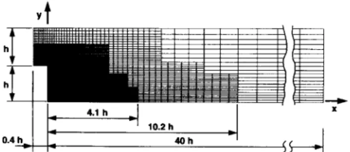
The shear stress was also experimentally determined. The exit section was placed at x = 40 h, with x measured from the expansion, as shown in Figure 3. This corresponds to a distance of approximately 5 reattachment lengths. At the exit section the streamwise gradients of the dependent variables are set to zero.

Preliminary calculations were performed using three different grids, without local grid refinement, and compris ing 40 x 20,80 x 40, and 160 X 80 control volumes. A fine grid was generated from a coarse one by dividing a control volume of the coarse grid into four smaller control vol-

Figure 3. Grid used to compute the flow over a backward-fac- ing step, with two levels of local grid refinement.

umes. The results computed using these grids allow an estimation of the solution error based on Richardson extrapolation, which helps to identify the regions where the grid should be refined. The solution error may be expanded in Taylor series yielding:

where 4 is the exact solution to the discretized equation, & is the approximate numerical solution obtained with grid spacing h, and Ed is the corresponding error. The coefficients a,, a2, _ . . may be functions of the coordinates but do not depend on h in the asymptotic range. If the grid spacing is doubled in both directions the solution error will be

e2,, = 4*,, - qb = 2a,h + 4a2h2 + ...

Subtracting these two series the difference between the two approximate numerical solutions is

+2h - +,, = a,h + 3a2h2 + ...

which is of the order of E,, for small h. If a second order discretization scheme is employed, the leading term of the series expansion is zero. Therefore the difference between the two numerical solutions is of the order of 3~,,

It is expected that the difference between the numerical solutions calculated using grids with 160 X 80 and 80 x 40 control volumes is a good estimation of the solution error in the finer grid for a first-order accurate method and a good estimation of three times the solution error in the finer grid for a second-order accurate method. The present calculations were carried out using the hybrid scheme, which reverts to the upwind scheme (first-order method) if the mesh Peclet number, Pe, is larger than two and reverts to central differences (second-order method) otherwise. Figure 4 shows the regions where [Pel < 2 and [Pel > 2 for both 160 X 80 and 80 X 40 grids. In the shaded region the central difference scheme was used for the finer grid (1 Pel < 2) and the upwind scheme was employed for the coarser grid (1 Pel > 2). The formal accuracy of the hybrid scheme lies between one and two. Therefore in the worst case (first-order accuracy) it is expected that the difference between the numerical solutions calculated using these two grids is a good estimation of the solution error in the finer grid.

The contours of the normalized differences between the numerical solutions obtained using 160 X 80 and 80 x 40 control volumes are plotted in Figure 5. The velocity components are normalized by the maximum inlet veloc-

IPel > 2 IPel < 2 _“)

I I I 1 I m

0.1 0.2 0.3 0.4 0.5 0.6 0.7 x

Figure 4. Contours of the Peclet number calculated using grids with 160X 80 and 80 x40 control volumes, without local re- finement. The shaded region indicates that lPeJ> 2 for the coarser grid and I/+ < 2 for the finer grid.

(6)

a)

0.1 02 0.3 0.4 0.5 0.6 u o.cQo 0.0050 o.w-30 0.0020 O.WlO 0.0005 0.1 0.2 0.3 0.4 0.5 0.6 u o.woo

cl

Figure 5. Contours of the normalized difference between the solutions obtained using 160 X 80 and 80 x 40 control volumes. (a) u-velocity; (b) v-velocity; and fc) turbulent kinetic energy.

ity, ua, and the turbulent kinetic energy is normalized by ~4;. The largest errors occur close to the corner of the step, proving that this is the region where local grid refinement is more effective.

Based on the above results a base grid with 40 X 20 control volumes and two levels of grid refinement was selected (see Figure 3). To generate this grid the normalized difference between the values of the dependent variables for the grids with 160 x 80 and 80 x 40 control volumes was considered. If the difference was larger than 6, two levels of grid refinement were used, and if the difference was between S and 6/2, only one level was used. In this problem, 6 was set equal to 0.015 for the u-velocity.

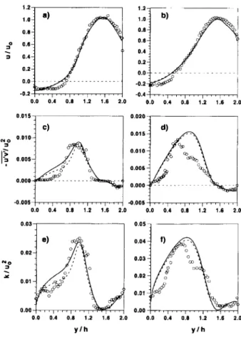
The predictions obtained using the locally refined grid and the standard grid with 160 X 80 control volumes are shown in Figure 6, along with the measurements.23 Figure 6 shows that similar results are obtained using the two different grids. Additional calculations were performed using a third level of grid embedding, but they are not presented here since the predictions are almost coincident to those shown. Therefore the numerical errors may be considered negligible compared to the differences between the measurements and the predictions. This is in agreement with the error estimation illustrated in Figure 5 and with the findings of Thangam and Hur,24 who con- cluded that a grid with 166 x 73 control volumes yielded results that were within acceptable limits for a similar configuration.

The predicted reattachment length is 7.6 h, 10% smaller than the measured value (8.5 h). This is consistent with the well-known behavior of the k-c model in these kinds of flo~s.~‘,~~ At x/h = 2 the mean axial velocity is in close agreement with the data outside of the recirculation region. In the recirculation region the velocity is underestimated near the velocity reversal locus, but it is overpre-

1.2 1.0 0.8 2 0.6 s 0.4 0.2 0.0 -0.2 0.0 0.4 0.8 1.2 1.6 2.0 0.015 0.010 0.005 0.000 -“.oosOW 1.6 2.0

-0.005

0.0

“““““172”;ls’

0.4 0.8 2.0

0.037 o.05_j

I 0.04 0.02 "," 0.03 Y 0.02 0.01 0.01 0.00 0.00 0.0 0.4 0.8 1.2 1.6 2.0 0.0 0.4 0.8 1.2 1.6 2.0 Y/h _y/h

Figure 6. Predicted (solid line, grid shown in Figure 3; dashed line, 160 x 80 control volumes without local grid refinement) and measured (symbols) normalized profiles for the backward-facing step flow. (a) u-velocity, x/h= 2; fb) u-velocity,

x/h=4; (cl shear stress, x/h=2; fd) shear stress, x/h=4; (e)

turbulent kinetic energy, x/h=2; and (f) turbulent kinetic energy,

x/h=4.

dieted close to the wall. At x/h = 4 the velocity is underpredicted in the recirculation region, indicating a smaller recirculating mass flow than the measured one. This is compensated by the slightly smaller velocities calculated in the upper channel half. These results are similar to those reported by Obi et a1.27

The shear stress is overpredicted in the recirculation region, both at x/h = 2 and at x/h = 4. This is a known shortcoming of the k-c model and is one of the main reasons for the underprediction of the reattachment length.2s Since the shear stress is responsible for the transfer of x-momentum in the y-direction the errors in the shear stress are related to the u-velocity errors mentioned above. The maximum predicted shear stress is located closer to the top wall than the measured value, and the peak is overpredicted at x/h = 4.

,2

No measurements of w are available. Hence the measured value of the turbulent _- kinetic energy was estimated by setting p= OS(u’= + p). Regarding this ap- proximation the predictions are in reasonable agreement with the measurements at x/h = 2 and x/h = 4. In the recirculation region the turbulent kinetic energy is overpredicted, similarly to the shear stress, suggesting that the main reason for the discrepancies observed in the shear

(7)

stresses, and accordingly in the mean velocity profiles, is caused by the wrong modelling of one of the terms of the turbulent kinetic energy equation.27

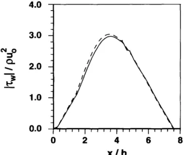
The predicted wall shear stress in the recirculation region is plotted in Figure 7. At the interface between the regions of different levels of refinement the wall shear stress profile exhibits a small kink. However it appears as a local discontinuity that does not influence the solution elsewhere.

Although the predictions shown in Figures 6 and 7 are very similar to each other the computational requirements are very different. The conventional grid (without local grid refinement) with 160 x 80 grid nodes requires 2,202 iterations and 1,909-see CPU time, in a DEC-2100 work- station, to achieve a converged solution, while the grid shown in Figure 3, with 4,707 grid nodes, requires only 1,273 iterations and 449 sec. These results and a few others are summarized in Table 2. All the results shown in this table were obtained using the following underrelaxation parameters: ‘Y, = LY,, = 0.75, (Ye = 0.25, and LQ = (Y,

= 0.7. The results show that the grid-embedding technique does not influence the convergence rate. Therefore the achievement of a given accuracy requires much less CPU time if local grid refinement is employed, due to the lower number of grid nodes, which are concentrated only where they are actually needed.

3.2 Flow over a square obstacle

The turbulent flow over a square obstacle in a plane channel, experimentally studied by Dimaczec et a1.,28 con- stitutes the second test case. The height of the channel (0.05 m) is twice the height of the obstacle (h = 0.025 m). The Reynolds number based on the maximum inlet velocity and on the height of the channel is 9.5 X 104. The measured profiles of both velocity components and turbu-

@Go

Q

$

-

4.0

3.0

2.0

1.0

0.0

0

2

4

6

8 x/h

Figure 7. Predicted wall shear stress (solid line, grid shown in

Figure 3; dashed line, 160 x 80 control volumes without local grid refinement).

Table 1. CPU time and number of iterations required to achieve convergence in the backward-facing step flow

Number of Number of CPU refinement grid Number of time Base grid levels nodes iterations (set)

40 x 20 0 776 583 29

40x20 1 1767 798 97

80 x 40 0 3075 1099 223

40 x 20 2 4707 1273 449

160X80 0 12359 2202 1909

lent kinetic energy at a distance of 0.4 h upstream of the obstacle were used as inlet boundary conditions. The dissipation rate at the inlet section was calculated using equation (12), and the measured turbulent shear stress profile. The exit section was placed at x = 21 h, with x measured from the leading edge of the obstacle, as shown in Figure 8. The streamwise gradients of the dependent variables are set to zero at the exit section.

An error estimation analysis similar to that described in the previous test case was carried out using three grids without local refinement and comprising 41 X 30, 82 X 60, and 164 x 120 grid nodes. The details of this analysis are omitted. Based on the results obtained, three grids with two or three levels of local refinement were selected, with the maximum concentration of grid nodes upstream and above the obstacle, and in the recirculating region downstream of the obstacle. One of the grids is shown in Figure 8. The base grid is identical to the grid without local refinement with 41 X 30 grid nodes. The local refinement was carried out by halving the control volumes in both directions. Therefore the second level of refinement corresponds to that of the grid with 164 X 120 control volumes and no local refinement. The finest refinement level corresponds to a grid with 328 X 240 grid nodes.

The reattachment length calculated using the grid displayed in Figure 8 is 7.38 h. This is close to the experi- mental value (7.12 h) and in agreement with the results of Kessler et a1.29

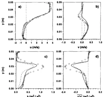
Figure 9 shows the comparison between the results obtained at section x/h = 0.08 using the grid with 164 x

120 control volumes and no local refinement, the grid shown in Figure 8 with three refinement levels and the measurements.28 This section is located over the obstacle, close to its leading edge. The predictions obtained using the two grids exhibit similar trends. However the peaks of the u-velocity, turbulent kinetic energy, and shear stress are closer to the measurements using the grid displayed in Figure 8. For this grid the peaks are underestimated by 9, 36, and 13%, respectively, while using the grid with 164 x 120 control volumes the peaks are underpredicted by 16, 46, and 23%, respectively.

The negative u-velocity close to the top face of the square obstacle indicates the presence of a thin recirculation zone. The .predicted maximum negative u-velocity exceeds the measured one. However the predicted maximum is closer to the wall than the first measured value. Therefore it is not possible to decide whether the observed discrepancy is due to the model or to the lack of measurements closer to the wall. However the displace-

(8)

h h

E

0.4h

+

0.05 0.05 0.04 0.04 0.03 0.03 E a. 0.02 0.02 0.01 0.01 0.00 0.00 -2 -1 0 1 2 3 4 5 -1.0 -0.5 0.0 0.5 1.0 ~(mw VW@ 0.05 - 0.05-

Figure 8. Grid used to compute the flow over a square obsta- cle, with three levels of local grid refinement.

ment of the predicted maximum reverse velocity toward the wall has also been observed in order-related flow configurations,” and it has been attributed to the turbulence model, although the reason for that behavior is not completely clear. Overall the u-velocity profile is in good agreement with the experimental one. This is also true for the u-velocity profile, although the peak velocity is underestimated, in agreement with the results of Kessler et a1.29 Both the experimental and the predicted turbulent kinetic energy and shear stresses are very small in the upper part of the channel. In the neighborhood of the top of the obstacle the turbulent kinetic energy rises sharply, but the predictions are unable to reproduce the peak. The shear stress increases, reaches a positive peak, and drops suddenly closer to the obstacle, reaching a negative peak. The model does not simulate satisfactorily this evolution.

Similar predictions are displayed in Figure 20 at section x/h = 2.0. This section is located downstream of the obstacle at a distance of one step height from its rear side. The predictions obtained using the locally refined grid are

0.025 k(dls2)

1

2.0 0.025 -0.4 -0.2 0.0 0.2 iG(m2/s2)

I

D 0.4

Figure 9. Predicted (solid line, grid shown in Figure 8; dashed line, 164 x 120 control volumes without local grid refinement) and measured (symbols) profiles for the flow over a square obstacle at x//1=0.08. (a) u-velocity; (b) v-velocity; (c) turbulent kinetic energy; and fd) shear stress.

a z.v

0.0 0.5 1.0 1.5 -0.4 -0.2 0.0 0.2 k(m2/s2) iT(m*/.s2)

Figure 10. Predicted (solid line, grid shown in Figure 8; dashed line, 164 x 120 control volumes without local grid refinement) and measured (symbols) profiles for the flow over a square obstacle at x/h=2. (a) u-velocity; (b) v-velocity; (c) turbulent kinetic energy; and (d) shear stress.

closer to the measurements than those computed without local grid refinement and 164 X 120 control volumes, especially in the recirculation region. However, both sets of predictions reveal well-known deficiencies of the k-c model. These include the prediction of a smaller recirculation mass flow, the maximum reversal u-velocity too close to the wall, and the underprediction of the turbulent kinetic energy and shear stress in the shear layer.

The CPU time and the number of iterations required to achieve convergence are given in Table 2. Besides the grids mentioned before, several other grids were considered, both with and without local refinement. All the calculations were performed using (Y, = (Y,, = (Ye = 0.5 and (Ye = (Y, = 0.7. Although both the number of iterations and the CPU time increase with the number of grid nodes, as expected, the increase is faster for the grids without local refinement. Therefore the local grid refinement yields an increase of the convergence rate, contrary to the behavior observed in test case 1 and in previous computations for laminar flows.18 The reason for this increase is not clear.

Table 2. CPU time and number of iterations required to achieve convergence in the flow over a square obstacle

Base grid

Number of Number of CPU refinement grid Number of time levels nodes iterations fsec)

41 x30 0 1080 1185 69 41 x30 1 3783 1537 446 82 x 60 0 4320 2764 778 41 x30 2 9555 1561 1087 164x 120 0 17220 4041 5388 41 x30 3 32043 2539 5715 41 x 30 3 39531 2601 8606

(9)

A possible explanation lies in the aspect ratio of the control volumes, defined as the ratio between their length and their height. Since the x = constant lines of the grid are expanding toward the exit section, the control volumes close to the exit section have high aspect ratios, especially close to y = h, achieving values of about 50. If local grid refinement is not used, the finer the grid, the larger will be the number of control volumes with high aspect ratio. But when local grid refinement is employed the number of cells with high aspect ratio does not change because the refinement is only carried out near the obstacle. There- fore the large number of cells with high aspect ratio used in grids without local refinement may be the reason for the observed marked decreased of the convergence rate for fine grids.

3.3 Flow in a sudden pipe expansion

The last problem studied here is the turbulent flow in an abruptly expanding circular pipe. The measurements of Moon and Rudinger3’ are used for evaluation purposes. The diameter of the pipe suddenly changes from d = 70 mm to D = 100 mm at the expansion (see Figure II). The Reynolds number based on the maximum velocity upstream of the expansion, where the flow is fully developed, is equal to 2.8 x 10’. The computational domain extends from x = - 0.2 D to x = 5 D and was selected after a few preliminary calculations in order to ensure that the loca- tion of the exit section does not influence the predictions. A fully developed turbulent velocity profile was prescribed at the inlet. The turbulent kinetic energy and the dissipation rate at the inlet were estimated following standard practices.25

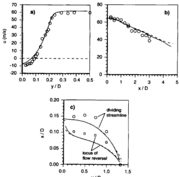
The results presented below were obtained using a grid with 60 x 40 control volumes, without local refinement, and the grid displayed in Figure 12 with three refinement levels. The local refinement was selected following an error estimation analysis as described in Section 3.1. The two numerical solutions are very close to each other and hardly are distinguishable in Figure 13.

The predicted reattachment length is 9.07 h using the grid without local refinement and 8.8 h using the grid presented in Figure 12. These compare favorably with the experimental value (8.8 h). This is consistent with other studies that have shown that, in contrast to the predictions of the backward-facing step flow, the standard k-c model predicts the reattachment length within the experimental uncertainty for the flow in a sudden pipe expansion.25

Figure 13(a) shows a radial profile of u-velocity close to the expansion, at x/D = 0.075. The predicted recircula-

0.2D

dj-+-+g;

*

\,6;jju

Figure 11. Configuration of the pipe with a sudden expansion.

Yt

‘3 1 0.2 *

-I

0.32 * 0.4 * c

Figure 12. Grid with three refinement levels used in the calcu- lation of the flow in a sudden pipe expansion.

tion zone is thinner and the absolute u-velocity is smaller than the measured ones. In the core of the pipe the predicted velocity profile closely follows the measured one. The decay of the u-velocity along the centerline is also in very good agreement with the measurements (Fig- ure 13[b]). However, both the dividing streamline that separates the recirculation zone from the main flow and the locus of flow reversal reveal that the predicted thick- ness of the recirculation zone is too small (see Figure

13[cl).

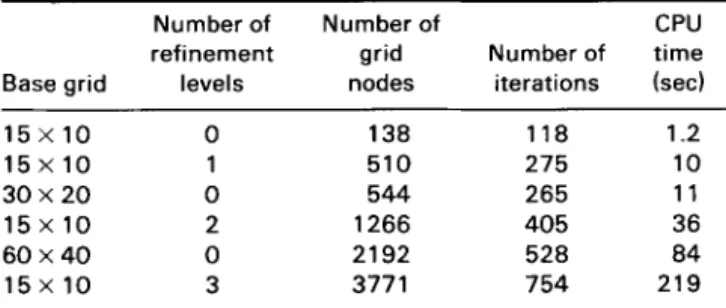
Finally, Table 3 shows the CPU time and the number of iterations required to achieve convergence using several grids, including those mentioned above. All these results were computed using LY, = (Y,, = 0.75, ap = 0.25, and (Ye = (Y, = 0.7. It can be seen that, as in the first test case, the convergence rate is not influenced by the local grid refinement. Therefore to achieve a given accuracy, CPU time can be saved using local grid refinement, be-

I

60

Figure 13. Predictions (solid line, grid shown in Figure 12; dashed line, 60 X 40 control volumes without local grid refine- ment) and measurements (symbols) for the flow in a sudden pipe expansion. (a) Radial profile of u-velocity at x/0=0.075; fb) u-velocity along the centerline; and k) dividing streamline and locus of the flow reversal.

(10)

Table 3. CPU time and number of iterations required to achieve convergence in the flow in a sudden pipe expansion

Number of Number of CPU refinement grid Number of time Base grid levels nodes iterations kec)

15x10 0 138 118 1.2 15x10 1 510 275 10 30x20 0 544 265 11 15x 10 2 1266 405 36 60x40 0 2192 528 84 15x10 3 3771 754 219

cause grid lines may be concentrated only where flow details need to be resolved. Hence the total number of grid nodes may be reduced. On another hand, for a prescribed number of grid nodes, better accuracy is achievable using local grid refinement, because more grid nodes may be placed in the flow regions where larger numerical errors are expected.

4. Conclusions

A grid-embedding technique formerly applied to the calculation of two-dimensional laminar incompressible flows was modified and extended to the modelling of turbulent recirculating flows. It employs a nonstaggered grid system with an arbitrary number of refinement levels. The method was applied to several turbulent flows using grids both with and without local grid refinement. The local grid refinement was placed in the regions where larger errors are expected, following an error estimation analysis based on Richardson extrapolation. From the analysis carried out the following conclusions may be drawn regarding the grid-embedding technique:

(9

(ii)

(iii)

(iv)

The modified treatment of the interfaces in the grid- embedding technique has been demonstrated in the simulation of turbulent flows.

The grid-embedding technique yields a significant reduction in the computing time, compared with standard grids, to achieve the same accuracy.

The grid-embedding technique enables an improve- ment of the solution accuracy if compared with standard grids using the same number of grid nodes. The advantages of the grid-embedding technique formerly reported for laminar flows are also observed for turbulent flows.

References

Chessire, G. and Henshaw, W. D. Composite overlapping meshes for the solution of partial differential equations. J. Comput. Phys.

1990, 90, 1-64 Rai, M. M. A Euler eauation

conservative treatment of zonal boundaries for calculations. J. Comput. Phys. 1986, 62, 472-503 Mitchel&ee, R. A., Salas, M. D., and HassaL, H. A. Grid embedding technique using Cartesian grids for Euler equations. AIAA .I.

1988, 26, 754-756

Bieterman, M. C., Bussoletti, .I. E., Hilmes, C. L., Johnson, F. T., Melving, R. G., and Young, D. P. An adaptive grid method for analysis of 3D aircraft configurations. Comput. Meth. Appl. Mech. Eng. 1992,101,225-249

5. Lapworth, B. L. Three-dimensional mesh embedding for the Navier-Stokes equations using upwind control volumes. Int. J. Num. Meth. Fluids 1993, 17, 195-220

6. Berger, M. J. and Jameson, A. Automatic adaptive grid refinement for the Euler equations. AIAA J. 1985, 23, 561-568 7. Davis, R. L. and Dannenhoffer, J. F. III. Three-dimensional

adaptive grid-embedding Euler technique. AIAA J. 1994, 32, 1167-1174

8. Kallinderis, V. G. and Baron, J. R. Adaptation methods for a new Navier-Stokes algorithm. AIAA J. 1989, 27, 37-43

9. Grasso, F., Marini, M., and Passalacqua, M. Viscous hiah-speed flow computations by adaptive mesh embedding techniques.

AIAA J. 1992,30, 1780-1788

10. Kallinderis, Y. and Vidwans, A. Generic parallel adaptive-grid Navier-Stokes algorithm. AIAA _I. 1994, 32, 54-61

11. Wanen, G. Application of multigrid and adaptive grid embedding to the two-dimensional flux-split Euler equations. Comm. Appl. Numer. Meth. 1992, 8, 771-784

12. van der Maarel, H. Adaptive multigrid for the steady Euler equations. Commun. Appl. Numer. Meth. 8, 1992, 771-784 13. Kotake, S. and Kodama, T. Coarse-fine mesh method for heat

and mass transfer in locally complex flows. ht. J. Num. Meth. Eng. 1988, 25, 347-355

14. de Lange, H. and de Goey, L. Numerical flow modelling in a locally refined grid. ht. J. Num. Meth. Eng. 1994, 37, 497-515 15. Thompson, M. C. and Ferziger, J. H. An adaptive multigrid

technique for the incompressible Navier-Stokes equations. J. Comput. Phys. 1989, 82, 94-121

16. Srinivasan, K. Segmented multigrid domain decomposition procedure for incompressible viscous flows. ht. J. Num. Meth. Fluids 1992, l&1333-1355

17. Bai, X. S. and Fuchs, L. Calculation of turbulent combustion of propane in furnaces. Int. J. Num. Meth. Fluids 1993, 17, 221-239 18. Coelho, P., Pereira, J. C. F., and Carvalho, M. G. Calculation of

laminar recirculating flows using a local non-staggered grid refinement system. Int. J. Num. Meth. Fluids 1991, 12, 535-557 19. Coelho, P. and Pereira, J. C. F. Calculation of a confined axisym-

metric laminar diffusion flame using a local grid refinement technique. Combust. Sci. Tech. 1993, 92, 243-264

20. Launder, B. E. and Spalding, D. B. The numerical computation of turbulent flows. Comput. Meth. Appl. Mech. Eng. 1974, 3, 269-289

21. Patankar, S. V. Numerical Heat Transfer and Fluid Flow. Hemi- sphere, Bristol, PA, 1980.

22 23. 24. 25. 26. 27. 28. 29. 30.

Majumdar, S. Role of underrelaxation in momentum interpolation for calculation of flow with non-staggered grids. Numer. Hear Trans. 1988, 13, 125-132

Durst, F. and Schmitt, F. Experimental studies of high Reynolds number backward-facing step flow. Proceedings of the 5th Sympo- sium on Turbulent Shear Flows, Cornell, Ithaca, NY, 1985, pp. 519-524

Thangam, S. and Hur, N. A highly resolved numerical study of turbulent separated flow past a backward-facing step. fnt. J. Eng. Sci. 1991, 29, 607-615

Nallasamy, M. Turbulence models and their applications to the prediction of internal flows: a review. Comput. Fluids 1987, 15, 151-194

Thangam, S. and Speziale, C. G. Turbulent flow past a backward-facing step: a critical evaluation of two-equation models. AIAA J. 1992, 30, 1314-1320

Obi, S., Peric, M., and Scheuerer, G. Finite volume calculations of a high Reynolds number backward facing step flow employing a colocated variable arrangement. ‘fransporf Phenomena in Turbu- lent Flows, eds. M. Hirata and N. Nasagi, Hemisphere, New York,

1988, pp. 633-647

Dimaczek, G., Kessler, R., Martinuzzi, R., and Tropea, C. The flow over two-dimensiorml surface-mounted obstacles at high Reynolds numbers. Proceedings of the 7th Symposium on Turbu- lent Shear Flows, Stanford University, Stanford, CA, 1989, pp. 10.1.1-10.1.6

Kessler, R., Peric, M., and Scheuerer, G. Solution error estimation in the numerical predictions of turbulent recirculating flows.

AGARD 1988, CP-437, pp. P9.1-Pg.12

Moon, L. F. and Rudinger, G. Velocity distribution in an abruptly expanding circular duct. J. Fluids Eng. 1977, 99, 226-230