"Economic Hardship, in relation to housing costs and ternure status

(1)

Economic Hardship, in Relation to Housing Costs and

Tenure Status: A study of Portugal

∗

Miguel Vian

†

11 de Setembro

Abstract

The primary goal of this study is to complement the literature on risk of poverty by looking at different household economic hardship indicators in relation to the housing cost burden. Housing costs are our focus on this study due to the weight that it was on the budget constraints of households and due to its status as a essential good, so much so that households which are burdened by housing costs will reduce most non-housing expenditure. We use data from the European Union Statistics on Income and Living Conditions dataset (EU-SILC) regarding Portugal from 2010 to 2014. Examining the influence of housing costs on household economic hardship we found that they are positively correlated. Also that higher education, better health, being married and having a higher income have a negative impact on the probability of households facing hardship. The probit method used brought us robust results but the model was susceptible to endogeneity. We used instrumental variable estimation to tackle the potential endogeneity of housing costs. The results of the models were insightful shedding some light into the complexities of poverty and its relation to housing costs.

Keywords: Housing cost burden, Tenure status, Poverty, Economic har-ship

∗_{I would like to thank everyone that supported me to come back and finish this important step of my}

life. I would especially like to give my thanks to professor Susana Peralta for her help and patience.

†_{Nova School of Business and Economics. Campus de Campolide, P-1099-032 Lisboa, Portugal. Email:}

(2)

List of Figures

List of Tables

1 Housing Costs . . . 5 2 Poverty indicators . . . 9

3 Poverty indicators as a percentage of households . . . 10

4 Summary statistics for all the variables . . . 13

(3)

6 financialpoverty and reportedpoverty with various determinants . . . 16

7 statpoverty with instrumental variables and first stage . . . 18

8 The three poverty indicators with tenure status . . . 19

9 Tenure status as a percentage of total households . . . 21

(4)

1 Introduction

The housing market crash due to the sub-prime crisis of 2007, mostly created from the artificially cheap supply of housing, left many countries dealing with its aftermath and showed many problems of having a lack of oversight in a market for such an essential asset. Today other problems are now on the forefront of housing. Such as the vacant house stories from cities like Toronto, where banks use houses only as ”secure” financial assets and gentrification where low income families are pushed to the ever increasing ur-ban sprawl and the ever higher prices that this phenomenon brings.

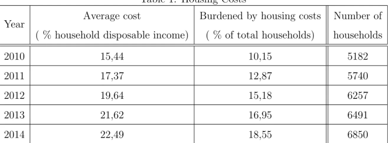
Housing makes up for a very important share of one’s income, as shown in Table 1, and therefore its costs may cause households to become so burdened1 _{that they reduce}

non-housing expenditures such as health care, education, food, and clothing.2.

Despite the fact that we do not do not know the poors’ preferences, we may reasonably guess that housing, clothing and food, which are the trifecta of basic human needs, should be included in any concept of poverty. Since populations started to grow in permanent geographic locations due to agriculture, leaving the nomadic lifestyle behind, housing has gained an ever increasing importance in human civilization and the lack of thereof more associated with poverty. As time passed the challenges of housing have changed. As pop-ulation density rises new problems are brought to the foreground. Cities in the beginning might have struggled with sanitation and victualling and now those seem like a trivial problems in the western world. But challenges still remain even if more nuanced and complex.

We use EU-SILC data for this study. The EU-SILC is a yearly European survey at, pub-lished by Eurostat, the household level that collects information such as income, debt, tax expenditures, health, social exclusion, household compositions,costs and characteris-tics even subjective questions about the perception of economic or social difficulties and housing costs. For the scope of this study we only use data that was collected after 2010 due to the fact that this was the first year where you could accurately collect detailed

1_{Households that pay more than 30% of gross income are considered burdened (US Department of}

Housing and Urban Development, Office of Policy Development and Research, 2007)

2_{Stone, M. E. (2006) What is housing affordability? The case for the residual income approach.}

(5)

Table 1: Housing Costs Year Average cost

( % household disposable income)

Burdened by housing costs ( % of total households) Number of households 2010 15,44 10,15 5182 2011 17,37 12,87 5740 2012 19,64 15,18 6257 2013 21,62 16,95 6491 2014 22,49 18,55 6850

data on the total housing costs. In this study we use three types of hardship indicators to get a wider outlook on different types of hardships that may arise from household budget problems. The first one is a indicator that combines income poverty3 _{with several}

mate-rial hardship indicators and also with the Eurostat’s definition of low work intensity, that allows us to go beyond solely monetary measures of poverty. The second refers to arrears on paying mortgage or rent, utility bills and other loans as a proxy for financial distress. The third one is a self-reported measure taken from the European Union Statistics on Income and Living Conditions dataset, more specifically, the answer to the question “A household may have different sources of income and more than one household member may contribute to it. Thinking of your household’s total income, is your household able to make ends meet, namely, to pay for its usual necessary expenses?”. We believe that this self reported measure is important due to some of the poverty factors that cannot be captured by the more monetary inclined EU-SILC questions and with this indicator we can shed some light on unobserved poverty risks within the household.

We follow Deida(2014) and pay particular attention to the differences between tenants and owners i.e. whether if the household is an outright owner, owner with mortgage, a renter, lives in a social housing project or receives its housing for free. The remainder of this paper is organized as follows: in section 2 we reference the various literature that relates poverty with housing costs, the various determinants of household hardship and the importance of tenure status for that same hardship; in section 3 we define, for this

3_{Based on the Eurofund Seminar Report on Working Poverty workers living in a household where at}

least one member works and where the overall income of the household (including social transfers and after taxation) remain below the poverty line (60 % of median equivalised income) are defined as poor.

(6)

study, poverty, the poverty lines and the different approaches to the subject; section 4 has the information related too the variables we are using , the models and the problems that arise from them; section 5 has the estimations and their interpretation; and finally, in section 6 we present some conclusions to the study.

2 Literature Review

There is an established empirical literature relates housing ot poverty most of the litera-ture uses measures of hardship that go beyond income based criteria (Nolan and Whelan 2011; Figari 2012; Fusco 2012). One example is Brandolini et al. (2013) who use five year long EU-SILC survey data to study the objective and subjective motives that affect households financial situation. In this paper they used a definition of financial hardship as a self reported measure of housing cost burden.

B´arcena-Mart´ın et al.(2013) use a poverty indicator that is based on household capacity to achieve some basic needs, like house warmth, eat protein every second day or enjoy a one week holiday, among others. Keeping with this line of reasoning they analysed household poverty level as a multidimensional indicator, using 2007 EU-SILC data, at both individual level and aggregate level. They found that institutional differences be-tween countries had a larger impact than individual household characteristics and also that income is only one of the many determinants of poverty. Factors such as education, housing status, and employment stability among others, would affect the probability of hardship as much as income.

This paper also relates to the literature on different determinants of hardship, Melzer(2011) studies the effects of pay-day loans on hardship and finds that improved access to credit increased the likelihood of households having difficulties in paying medical bills, mortgage payments and utility bills.

Other example is Mimura(2008) who studies the impact of housing costs and poverty on the economic hardships of low income families. Using data available in the National Survey of America’s Families, she crafted an indicator based on a factor score of several economic hardship items, concluding that housing cost burden had a smaller impact than poverty status.

(7)

Further, in the same context, there are some works that emphasize the impact of tenure status on household hardship. Conley and Gifford (2006) studied the relation between so-cial spending and house ownership. And found that in countries where the first was lower the latter was seen as substitute for social insurance. Watson and Webb (2009) in their paper highlight the importance of controlling for tenure status when studying poverty. By regressing household ownership in a model for reported hardship they observed that home owners are less likely to report difficulties. Furthermore by analysing cross country data they identified that in countries with high home ownership the relative poverty level is higher. Meaning that in countries with greater income discrepancies the idea of owning a house is used as an insurance.

A recent paper by Deida(2014) is very close to our analysis in the following aspects: We use the three hardship indicators, the housing costs and burden variables and the most of the modelling approach used by the author. However we depart from Deida in a number of important ways as per example, we do not cut out the elderly nor the unemployed from our data set, we use all the tenure statuses available from the EU SILC survey, leaving in the households on social housing and free accommodation, we also analyse various years, spilt education levels to get a detailed information on the impacts of education and only analyse one country.

3 Methodological review

The above collection of studies mirror well a concern that Ravallion (2015) exposes about poverty and poor people. That the heterogeneity of characteristics of the poor and the influence of such complexity on their utility functions cannot be explained by observable supply and demand behaviours. Meaning that until we have perfect information new assumptions will be made about what means to be poor and this in turn will bring new light into this discussion.

In this paper we try to define poverty by having a multi dimensional approach to the subject. We do this by using three hardship indicators as a proxies for poverty lines. The multi dimensionality come from the fact that the indicators have different components, some income and material based and others subjective. With this method we should

(8)

overcome some of the limitations of a uni-dimensional approach. And thus better reflect the complex topic that is poverty and its measurement.

4 Data and Methodology

The data used in this research project is taken from the European Union Statistics on Income and Living Conditions. We use cross sectional EU-SILC between 2010 and 2014, the period in which Eurostat started to include housing and mortgage related in the sur-veys. More recent data was not available.

The samples vary between 5182 households surveyed for 2010 and 6850 for 2014, with information on demographic and socio-economic characteristics at the household and in-dividual levels, for Portugal only. Given that household members share the same burdens of housing costs (Cantillon and Nolan 1998), we use household level data by selecting a representative member of the household.

We implement the following regressions: two probit models for each of the three hardship indicators, as the dependent variables, with one linear probability model for robustness; a linear instrumental variable estimation with a baseline regression; and three probit models for the hardship indicators with tenure status. The various regressions are to be compared to a baseline regression present the first probit models.

4.1 Poverty indicators

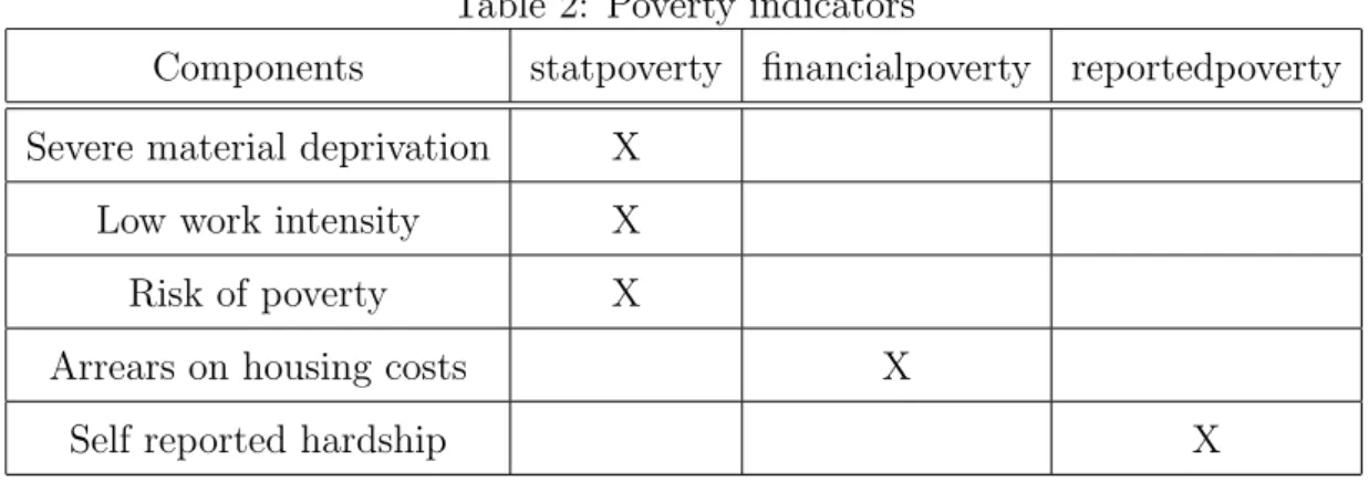
One of the many strong points of using the EU-SILC, in the dates selected, is that all of information that is required to make different poverty indicators can be found with the multitude of questions asked in the survey. The components for each of the poverty indicators used in the study are as follows: Firstly we have statpoverty that is a dummy variable that turns 1 when the household has experienced at least one of the three situations of severe material deprivation, low work intensity and/or risk of poverty. This indicators follows the Eurostat definitions of poverty by looking at severe material deprivation that consists on a state where a household fails to afford at least four of the following nine items; one week’s holiday away from home; a meal with meat, chicken, fish or vegetarian equivalent every second day; unexpected financial expenses; a telephone

(9)

Table 2: Poverty indicators

Components statpoverty financialpoverty reportedpoverty Severe material deprivation X

Low work intensity X Risk of poverty X

Arrears on housing costs X

Self reported hardship X

(including mobile telephone); a colour TV; a washing machine; a car; and heating to keep the home adequately warm. Severe material deprivation exists only if the household does not have the item due to its affordability4_{. Low work intensity was defined as households}

where the lead person worked less than 20 percent of their total potential during the year of the study, i.e. unemployed more than 10 months on the respective year of the survey. Risk of poverty is considered if the household’s equivalised disposable income is at 60 per cent of the national median equivalised disposable income after social transfers5_.

Secondly we have financialpoverty, a dummy variable, that focuses more on the financial side of poverty. This indicator turns 1 if households have inability to afford at least one of the following items in the last 12 months: utility bills, mortgage or rent payments and/or hire purchase instalments or other loans.

Finally we have reportedpoverty, also a dummy variable, that is the self reported poverty indicator. As stated before some facets of poverty cannot be fully observed only by the income and material based questions presented in the EU-SILC. So for this indicator we are using a question from the EU-SILC survey where households were asked to reply to the following question: “A household may have different sources of income and more than one household member may contribute to it. Thinking of your household’s total income, is your household able to make ends meet, namely, to pay for its usual necessary expenses?” the dummy turns 1 for households that replied “with great difficulty”.

4_{An example of such a difference is that some households might have someone who is afraid of air}

travel so they don not go on holiday

5_{The equivalised disposable income is the total income of a household, after tax and other deductions,}

that is available for spending or saving, divided by the number of household members converted into equalised adults

(10)

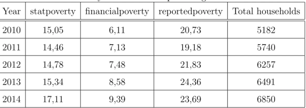
Table 3: Poverty indicators as a percentage of households

Year statpoverty financialpoverty reportedpoverty Total households

2010 15,05 6,11 20,73 5182

2011 14,46 7,13 19,18 5740

2012 14,78 7,48 21,83 6257

2013 15,34 8,58 24,36 6491

2014 17,11 9,39 23,69 6850

Table 3 shows the percentages of households affected by each of this poverty indicators in the different years

4.2 Housing cost indicators

To be able to study the indicators of poverty in relation to housing its now important to define measurements of housing cost burden. We use two variables: HC is the actual housing cost supported by households in relation to that same household’s equivalised income. In the case of home owners, housing costs would include the mortgage payment (principal and interest), property taxes, insurance, utilities, and maintenance costs. For tenants these costs include utilities and monthly rent. HBU is a self-reported statistic where the household representative is asked “Please think your total housing costs includ-ing mortgage repayment (instalment and interest) or rent, insurance and service charges (sewage removal, refuse removal, regular maintenance, repairs and other charges). To what extent are these costs a financial burden to you?” and if they respond “A heavy burden” then this dummy variable is assigned the value of 1.

4.3 Determinants of poverty

The probit model is used as the main model due to its advantage of the predicted values being in the unit range, since our dependent variables are all dummies. The model takes the form:

(11)

P r(H1i = 1 | X) = Φ(Xθβ)

Where P r denotes probability, and Φ is the Cumulative Distribution Function (CDF) of the standard normal distribution. The parameters β are typically estimated by maximum likelihood.

4.3.1 Causal effects of housing costs

The endogeneity might come from the characteristics of the household, like number of children or older people in the household, or even from different needs that arise from such characteristics, like needing easier access to better services like schools or hospitals. Another problem is that the perception of hardship may depend on the household finan-cial status, wealthier people have a different perception of hardship than poorer people, possibly leading to a reverse causality problem Ideally one would estimate an IV pro-bit. However, due to a computational difficulties we opted for the linear two-stage least squares estimation.The model is expressed by:

H1i = βZi+ π ˆCi+ εi

Ci = γZi+ α1Instrument1+ α2Instrument2+ υi

According to Angrist and Pischke (2008) the difference between the maximum likelihood estimation or the two least squares in empirical data is small enough to be ignored as long as we assume that we are estimating local average treatment effects. As for the biased 2SLS estimation we do not discard the hypotheses that the instruments are correlated to the error term but due to lack of better uncorrelated data, like regional credit access. But the large sample size and the small total number of instruments should fix some of that bias.

4.3.2 Other effects on hardship

The set of demographic indicators included age, education, a dummy indicating household being married, a dummy for single parents, a dummy for childless couples, a variable re-lated to the number of children in the household, and a dummy corresponding to a question

(12)

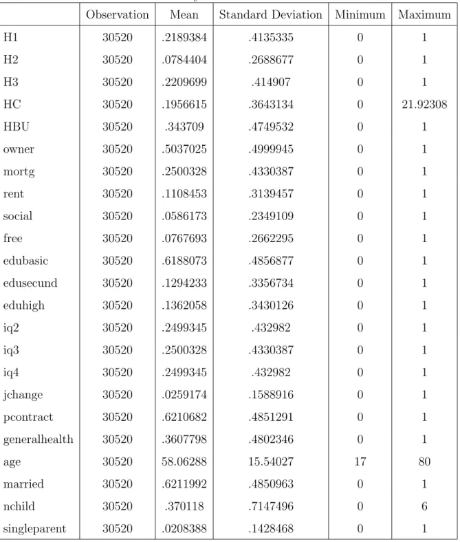
on the survey asking if the household reports good health. For more economic variables we have income quartile dummies. In terms of education we divided the households into categorical variables, each corresponding to the highest level of education achieved by the household, lack of education, only primary education edubasic , secondary education edusecund and tertiary education or higher eduhigh. Further, to also reflect influences from the labour market a set of variables regarding the job of the lead of the household are going to be used, a dummy indicating whether the household head had a permanent contract, and a dummy indicating change of job with respect to the previous year. And finally a series of year dummies to capture unobservable macroeconomic effects that im-pact household poverty. The summary statistics of all the variables used are shown in Table 4.

5 Empirical Estimation

5.1 Determinants

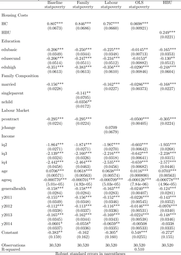
Results about the determinants of hardship are present in Tables 5.1 and 6. Firstly we are going to estimate probit equations with one of our three poverty indicators as the dependent variable, in this case statpoverty, with Housing Costs (HC), demographic and socio-economic variables, this will be our baseline regression where we will try to draw some meaningful comparisons. Then we linearly regress this baseline regression to confirm the robustness our results. And finallystatpoverty is regressed using probit with our other housing costs indicator HBU.

The estimated coefficients in Table 5.1 have the expected signs, the education variables have negative sign meaning that acquiring a higher education puts households at less risk of being in hardship conditions. The same analysis can be made about income quartiles. As expected being healthy also reduces risk of poverty. In relation to the age statistic it appears that as the household gets older they have an increased risk but by looking at the value for age squared the effect of age on poverty reduces as time passes. Housing cost is positively correlated with the probability of facing hardship in both the objective (HC ) and subjective (HBU ) indicators. In terms of family composition

(13)

Table 4: Summary statistics for all the variables

Observation Mean Standard Deviation Minimum Maximum

H1 30520 .2189384 .4135335 0 1 H2 30520 .0784404 .2688677 0 1 H3 30520 .2209699 .414907 0 1 HC 30520 .1956615 .3643134 0 21.92308 HBU 30520 .343709 .4749532 0 1 owner 30520 .5037025 .4999945 0 1 mortg 30520 .2500328 .4330387 0 1 rent 30520 .1108453 .3139457 0 1 social 30520 .0586173 .2349109 0 1 free 30520 .0767693 .2662295 0 1 edubasic 30520 .6188073 .4856877 0 1 edusecund 30520 .1294233 .3356734 0 1 eduhigh 30520 .1362058 .3430126 0 1 iq2 30520 .2499345 .432982 0 1 iq3 30520 .2500328 .4330387 0 1 iq4 30520 .2499345 .432982 0 1 jchange 30520 .0259174 .1588916 0 1 pcontract 30520 .6210682 .4851291 0 1 generalhealth 30520 .3607798 .4802346 0 1 age 30520 58.06288 15.54027 17 80 married 30520 .6211992 .4850963 0 1 nchild 30520 .370118 .7147496 0 6 singleparent 30520 .0208388 .1428468 0 1

(14)

Table 5: statpoverty with various determinants and OLS robustness check

Baseline Family Labour OLS HBU statpoverty statpoverty statpoverty statpoverty

Housing Costs HC 0.807*** 0.846*** 0.797*** 0.0698*** (0.0673) (0.0686) (0.0660) (0.00921) HBU 0.249*** (0.0221) Education edubasic -0.206*** -0.250*** -0.225*** -0.0145** -0.165*** (0.0349) (0.0344) (0.0348) (0.00713) (0.0353) edusecund -0.206*** -0.247*** -0.234*** -0.0153* -0.130** (0.0514) (0.0511) (0.0512) (0.00882) (0.0512) eduhigh -0.351*** -0.383*** -0.356*** -0.0290*** -0.248*** (0.0613) (0.0613) (0.0610) (0.00846) (0.0604) Family Composition married -0.156*** -0.162*** -0.0286*** -0.168*** (0.0228) (0.0227) (0.00373) (0.0227) singleparent -0.141** (0.0705) nchild -0.0356** (0.0172) Labour Market pcontract -0.295*** -0.295*** -0.0500*** -0.305*** (0.0224) (0.0224) (0.00405) (0.0224) jchange 0.0709 (0.0679) Income iq2 -1.864*** -1.874*** -1.907*** -0.603*** -1.935*** (0.0271) (0.0271) (0.0270) (0.00642) (0.0268) iq3 -2.139*** -2.160*** -2.216*** -0.642*** -2.238*** (0.0324) (0.0326) (0.0318) (0.00641) (0.0315) iq4 -2.442*** -2.464*** -2.535*** -0.659*** -2.577*** (0.0458) (0.0463) (0.0456) (0.00682) (0.0446) age 0.0706*** 0.0618*** 0.0638*** 0.0116*** 0.0703*** (0.00571) (0.00563) (0.00574) (0.000890) (0.00563) agesq -0.000770*** -0.000701*** -0.000709*** -0.000126*** -0.000778***

(5.01e-05) (4.92e-05) (5.03e-05) (7.84e-06) (4.96e-05) generalhealth -0.158*** -0.158*** -0.163*** -0.0240*** -0.124*** (0.0284) (0.0284) (0.0283) (0.00407) (0.0281) y2011 -0.155*** -0.156*** -0.152*** -0.0226*** -0.143*** (0.0349) (0.0348) (0.0346) (0.00545) (0.0352) y2012 -0.112*** -0.113*** -0.116*** -0.0146*** -0.0976*** (0.0338) (0.0337) (0.0336) (0.00531) (0.0340) y2013 -0.165*** -0.162*** -0.169*** -0.0224*** -0.148*** (0.0345) (0.0344) (0.0343) (0.00538) (0.0346) y2014 -0.0601* -0.0558* -0.0659** -0.00508 -0.0338 (0.0337) (0.0336) (0.0335) (0.00533) (0.0335) Constant -0.383** -0.162 -0.305* 0.548*** -0.272* (0.159) (0.162) (0.160) (0.0255) (0.155) Observations 30,520 30,520 30,520 30,520 30,520 R-squared 0.510

(15)

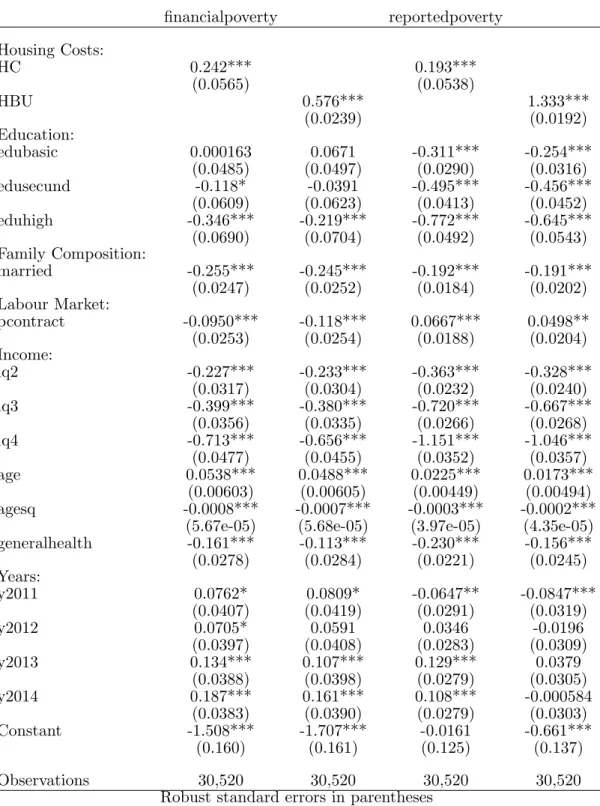
it seems that being married helps the household but on the other hand the negative sign on single parent dummy and on the number of children imply something that goes against what we expected. Finally for the labour statistics we observe that having a permanent contract is a boon for the household while having a job change in the last year is not statistically significant. In columns 2 and 3 we use alternate indicators for labour and family compositions for comparisons and robustness. As it is clear from Table 5.1, the coefficients that are not removed do not change sing nor significance, hence we conclude that out specification is robust. In the next table we are regressing each of our other two poverty indicators, financialpoverty and reportedpoverty, with our housing costs variables and with the other determinants used in the baseline regression. In Table 5 the similarities are apparent to our baseline, with one notable exception, it appears that having basic education level is not statistically significant to having arrears on utilities, mortgages or other loans.

5.2 IV regression

As discussed in section 4.3.1 there are reasons to believe that there will be endogeneity. These issues merit the use of and IV probit regression. We follow Deida(2014) by using the same EU-SILC variables as instruments. To use the instrument variables we assume that house size and location are correlated to housing costs. These variables are going to be instruments of HC and HBU and they are dummies indicating whether the number of rooms was smaller than four dhsize and an interaction term between urban location and the presence of noise urbnoise. The rationale is that a bigger house would cost more than a smaller one and if there were enough savings , in housing, a family would decide to move to a noisier area. The next Table 7 show us the results of IV regression and its correspondent first stage estimation.6

Analysing the results of the firsts stage estimation we observe that one of the instruments in not statistically significant, while the urbnoise has a positive impact, a good F-statistic value, a positive sigh for education levels and house costs and also a positive sign for the health indicator. For the IV regression in Table 7, the sub population that has small number of rooms and is affected by urban noise, we verify that housing costs still influences

(16)

Table 6: financialpoverty and reportedpoverty with various determinants financialpoverty reportedpoverty Housing Costs: HC 0.242*** 0.193*** (0.0565) (0.0538) HBU 0.576*** 1.333*** (0.0239) (0.0192) Education: edubasic 0.000163 0.0671 -0.311*** -0.254*** (0.0485) (0.0497) (0.0290) (0.0316) edusecund -0.118* -0.0391 -0.495*** -0.456*** (0.0609) (0.0623) (0.0413) (0.0452) eduhigh -0.346*** -0.219*** -0.772*** -0.645*** (0.0690) (0.0704) (0.0492) (0.0543) Family Composition: married -0.255*** -0.245*** -0.192*** -0.191*** (0.0247) (0.0252) (0.0184) (0.0202) Labour Market: pcontract -0.0950*** -0.118*** 0.0667*** 0.0498** (0.0253) (0.0254) (0.0188) (0.0204) Income: iq2 -0.227*** -0.233*** -0.363*** -0.328*** (0.0317) (0.0304) (0.0232) (0.0240) iq3 -0.399*** -0.380*** -0.720*** -0.667*** (0.0356) (0.0335) (0.0266) (0.0268) iq4 -0.713*** -0.656*** -1.151*** -1.046*** (0.0477) (0.0455) (0.0352) (0.0357) age 0.0538*** 0.0488*** 0.0225*** 0.0173*** (0.00603) (0.00605) (0.00449) (0.00494) agesq -0.0008*** -0.0007*** -0.0003*** -0.0002***

(5.67e-05) (5.68e-05) (3.97e-05) (4.35e-05) generalhealth -0.161*** -0.113*** -0.230*** -0.156*** (0.0278) (0.0284) (0.0221) (0.0245) Years: y2011 0.0762* 0.0809* -0.0647** -0.0847*** (0.0407) (0.0419) (0.0291) (0.0319) y2012 0.0705* 0.0591 0.0346 -0.0196 (0.0397) (0.0408) (0.0283) (0.0309) y2013 0.134*** 0.107*** 0.129*** 0.0379 (0.0388) (0.0398) (0.0279) (0.0305) y2014 0.187*** 0.161*** 0.108*** -0.000584 (0.0383) (0.0390) (0.0279) (0.0303) Constant -1.508*** -1.707*** -0.0161 -0.661*** (0.160) (0.161) (0.125) (0.137) Observations 30,520 30,520 30,520 30,520

Robust standard errors in parentheses *** p<0.01, ** p<0.05, * p<0.1

(17)

hardship in the same way as in the baseline regression and the other determinants remain, also, unchanged. Ideally in future work we would use regular IV probit with better available instruments. It is important to be able to study the poverty phenomena without the complications of endogeneity on the studies made.

5.3 Household Hardship and Tenure Status

As other works have showed that tenure status exerts a big influence upon households. We now move to analysis on the choices of tenure status among the Portuguese survey population and how they relate to economic hardship and housing costs. Tenure is impor-tant because housing is a long term investment that families value as a buffer for unseen contingencies, as a safety net for retirement and old age and as a real asset with a more personal utility than other assets. The importance is compounded by the financial and social consequences that the household must face due to that same tenure status choice. There is a trade off between tenure choices.

For the empirical estimation using tenure status we create one dummy variables for each type of tenure status available on EU-SILC. We first start with owner where it takes the value 1 if the household is a outright owner of a house, mortg for households who are owners but paying mortgage, social for people who live is discounted rent or social habitation and free for those agents that their accommodation is provided free. We now re estimated the probit regressions with our hardship indicators as dependent variables and with our new tenure status independent variables leaving out rent, that is a dummy for a tenant, in order to have a comparison to other tenure statuses.

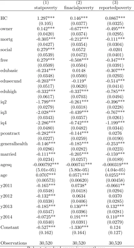
In the first table 8 we observe that or probit model has captured some unexpected but interesting effects of tenure status on hardship. It seems that going from a tenant to an outright owner leads to an increase of the probability of hardship, while having a mortgage while owning a house has a negative probability effect on hardship. This is not the case when we use financialpoverty or reportedpoverty. For the cases of free and social we see variations on the signs and on the significance levels across the three regressions. The rest of descriptive statistics do not alter from our baseline except for edubasic on the second column and pcontract on the third column that are both non statistically significant. The

(18)

Table 7: statpoverty with instrumental variables and first stage (1) (2) First stage 2SLS HC statpoverty dhsize 0.00379 (0.00448) urban 0.0468*** (0.00429) HC 0.498*** (0.0847) edubasic 0.0421*** -0.0343*** (0.00717) (0.00781) edusecund 0.0696*** -0.0484*** (0.00963) (0.0112) eduhigh 0.0510*** -0.0549*** (0.0101) (0.0108) iq2 -0.171*** -0.530*** (0.00567) (0.0154) iq3 -0.225*** -0.547*** (0.00594) (0.0197) iq4 -0.284*** -0.539*** (0.00669) (0.0245) pcontract -0.0255*** -0.0413*** (0.00439) (0.00447) generalhealth 0.0129*** -0.0300*** (0.00495) (0.00483) married -0.0103** -0.0223*** (0.00435) (0.00425) age -0.00137 0.0122*** (0.00103) (0.000977) agesq -1.90e-05** -0.000118*** (9.03e-06) (8.69e-06) y2011 0.0186*** -0.0305*** (0.00659) (0.00641) y2012 0.0395*** -0.0315*** (0.00647) (0.00696) y2013 0.0574*** -0.0469*** (0.00642) (0.00777) y2014 0.0645*** -0.0327*** (0.00636) (0.00812) Constant 0.433*** 0.360*** (0.0287) (0.0459) F 225.9 1570

Instruments: dhsize; urbnoise

Observations 30,520 30,520 R-squared 0.112 0.384

Standard errors in parentheses *** p<0.01, ** p<0.05, * p<0.1

(19)

Table 8: The three poverty indicators with tenure status

(1) (2) (3)

statpoverty finacialpoverty reportedpoverty HC 1.297*** 0.146*** 0.0867*** (0.105) (0.0377) (0.0325) owner 0.142*** -0.677*** -0.495*** (0.0420) (0.0374) (0.0295) mortg -0.305*** -0.212*** -0.111*** (0.0427) (0.0354) (0.0304) social 0.279*** 0.0572 -0.0201 (0.0539) (0.0472) (0.0401) free 0.279*** -0.508*** -0.347*** (0.0509) (0.0504) (0.0391) edubasic -0.234*** 0.0148 -0.307*** (0.0348) (0.0500) (0.0293) edusecund -0.203*** -0.119* -0.514*** (0.0517) (0.0620) (0.0414) eduhigh -0.332*** -0.337*** -0.785*** (0.0617) (0.0703) (0.0494) iq2 -1.799*** -0.261*** -0.396*** (0.0279) (0.0318) (0.0228) iq3 -2.028*** -0.439*** -0.767*** (0.0343) (0.0357) (0.0261) iq4 -2.286*** -0.742*** -1.199*** (0.0480) (0.0482) (0.0344) pcontract -0.282*** -0.144*** 0.0276 (0.0227) (0.0259) (0.0190) generalhealth -0.146*** -0.185*** -0.253*** (0.0286) (0.0282) (0.0223) married -0.111*** -0.205*** -0.159*** (0.0234) (0.0257) (0.0189) agesq -0.000792*** -0.000741*** -0.000319***

(5.01e-05) (5.80e-05) (4.04e-05) age 0.0707*** 0.0571*** 0.0255*** (0.00573) (0.00620) (0.00458) y2011 -0.165*** 0.0738* -0.0661** (0.0348) (0.0418) (0.0294) y2012 -0.132*** 0.0634 0.0370 (0.0338) (0.0406) (0.0285) y2013 -0.185*** 0.130*** 0.132*** (0.0347) (0.0396) (0.0281) y2014 -0.0725** 0.191*** 0.110*** (0.0340) (0.0391) (0.0279) Constant -0.527*** -1.330*** 0.124 (0.162) (0.164) (0.127) Observations 30,520 30,520 30,520

(20)

lack of robust results on this table might mean some unobserved effects are taking place that are not captured by our models. But we still can see that housing costs are related to economic hardship.

6 Conclusions

In this paper we tried to shed some light on the relationship between housing costs and economic hardship. Using recent literature on poverty, that motivated us to use non income and self reported statistics, we found some expected effects. The linkage between various poverty measures and both objective and subjective housing burden seems to be positively correlated. The addition of tenure status in to the baseline regression showed us some new correlations between hardship and tenure status that are intriguing but house costs and the other determinants stay robust with our baseline regression. We found endogeneity on our models and used the linear IV model to address this issue with some success by having similar coefficients to our baseline estimation.

We would like to comment that this exercise was a great opportunity of getting to know more of the recent poverty literature and how that field of study is evolving and finding new methods to answer old questions. The EU-SILC survey is a powerful tool in this aspect and we hope that in the future data collection on the more economic vulnerable only gets wider, more diverse and more personal so we can better understand this phenomena and help attenuate its effects. In a final note related to the particularities of Portuguese housing market we think it is important to refer that there is serious difficulty to find house pricing information on national levels, meaning, that further detailed research, on topics related to housing and its effects on Portuguese families and economy, is severely dwindled. This could be addressed by the Instituto Nacional de Estatistica with the creation of a database on such topics, or just getting a new country specific annex in the EU-SILC survey to that effect with self reported question about house prices.

(21)

7 Appendix

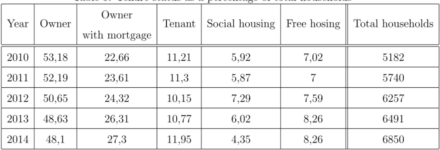
Table 9: Tenure status as a percentage of total households Year Owner Owner

with mortgage

Tenant Social housing Free hosing Total households

2010 53,18 22,66 11,21 5,92 7,02 5182

2011 52,19 23,61 11,3 5,87 7 5740

2012 50,65 24,32 10,15 7,29 7,59 6257

2013 48,63 26,31 10,77 6,02 8,26 6491

2014 48,1 27,3 11,95 4,35 8,26 6850

(22)

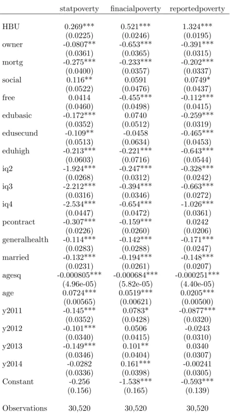
Table 10: Poverty indicators with tenure status and subjective housing costs

statpoverty finacialpoverty reportedpoverty HBU 0.269*** 0.521*** 1.324*** (0.0225) (0.0246) (0.0195) owner -0.0807** -0.653*** -0.391*** (0.0361) (0.0365) (0.0315) mortg -0.275*** -0.233*** -0.202*** (0.0400) (0.0357) (0.0337) social 0.116** 0.0591 0.0749* (0.0522) (0.0476) (0.0437) free 0.0414 -0.455*** -0.112*** (0.0460) (0.0498) (0.0415) edubasic -0.172*** 0.0740 -0.259*** (0.0352) (0.0512) (0.0319) edusecund -0.109** -0.0458 -0.465*** (0.0513) (0.0634) (0.0453) eduhigh -0.213*** -0.221*** -0.643*** (0.0603) (0.0716) (0.0544) iq2 -1.924*** -0.247*** -0.328*** (0.0268) (0.0312) (0.0242) iq3 -2.212*** -0.394*** -0.663*** (0.0316) (0.0346) (0.0272) iq4 -2.534*** -0.654*** -1.026*** (0.0447) (0.0472) (0.0361) pcontract -0.307*** -0.159*** 0.0242 (0.0226) (0.0260) (0.0206) generalhealth -0.114*** -0.142*** -0.171*** (0.0283) (0.0288) (0.0247) married -0.132*** -0.194*** -0.148*** (0.0231) (0.0261) (0.0207) agesq -0.000805*** -0.000684*** -0.000251***

(4.96e-05) (5.82e-05) (4.40e-05) age 0.0724*** 0.0519*** 0.0205*** (0.00565) (0.00621) (0.00500) y2011 -0.145*** 0.0783* -0.0877*** (0.0352) (0.0428) (0.0320) y2012 -0.101*** 0.0506 -0.0243 (0.0340) (0.0415) (0.0310) y2013 -0.149*** 0.101** 0.0340 (0.0346) (0.0404) (0.0307) y2014 -0.0282 0.161*** -0.00241 (0.0336) (0.0398) (0.0305) Constant -0.256 -1.538*** -0.593*** (0.156) (0.165) (0.139) Observations 30,520 30,520 30,520

(23)

8 Bibliography

References

[1] Angrist, J. and Pischke, J. (2008). Mostly harmless econometrics: An empiricist’s companion. Princeton Univ Pr.

[2] B´arcena-Mart´ın, E., Lacomba, B., Moro-Egido, A. I., and P´erez- Moreno, S. (2013). Country differences in material deprivation in Europe. Review of Income and Wealth: Advance online publication. doi:10.1111/roiw.12030.

[3] Brandolini, M., Coroneo, F., Giarda, E., and Moriconi, C., and See, S.G. (2013). Differences in perceptions of the housing cost burden among European countries (Nota di lavoro Prometeia 2010-01). Retrieved from Prometeia website: http://www.prometeia.it/it-it/ricerca/note-di-lavoro.aspx?idC=63274&LN=it-IT. [4] Cantillon, S., and Nolan, B. (1998). Are married women more deprived than their

husbands? Journal of Social Policy, 27(02), 151?171.doi:10.1017/s0047279498005261. [5] Conley, D., and Gifford, B. (2006). Home ownership, social insurance, and the welfare

state. In Sociological Forum, 21, 55?82. doi:10.1007/s11206-006-9003-9.

[6] Deida, Manuela (2014) Economic Hardship, Housing Cost Burden and Tenure Status: Evidence from EU-SILC DOI: 10.1007/s10834-014-9431-2

[7] Figari, F. (2012). Cross-national differences in determinants of multiple deprivation in Europe. The Journal of Economic Inequality, 10(3), 397?418. doi:10.1007/s10888-010-9157-9.

[8] Fusco A., (2012) The relationship between income and housing deprivation in Lux-embourg: a longitudinal analysis (Working Paper Series 2012-10). Retrieved from CEPS/INSTEAD website: http://www.ceps.lu/?type=module&id=104&tmp=1822. [9] Melzer, B. T. (2011). The real costs of credit access: Evidence from the

payday lending market. The Quarterly Journal of Economics, 126(1), 517?555. doi:10.1093/qje/qjq009.

(24)

[10] Mimura, Y. (2008). Housing cost burden, poverty status, and economic hardship among low-income families. Journal of Family and Economic Issues, 29(1), 152?165. doi:10.1007/s10834-007-9085-4.

[11] Nolan, B., and Whelan, C. T. (2011). Poverty and deprivation in Europe, OUP Catalogue. Oxford: Oxford University Press

[12] Ravallion, Martin. (2015). The Economics of Poverty (pp. 131?289)

[13] Stone, M. E. (2006) What is housing affordability? The case for the residual income approach. Housing Policy Debate, 17(1),151?184. doi:10.1080/10511482.2006.9521564. [14] Venti, S. F., and Wise, D. A. (2004). Ageing and housing equity: another look. Wealth portfolios in the US and the UK. In D. Wise (Ed.),Perspectives on the economics of ageing.(pp. 127?175). Chicago: Chicago University Press.

[15] Watson, D., and Webb, R. (2009) Do Europeans view their homes as castles? Home-ownership and poverty perception throughout Europe. Urban Studies, 46(9), 1787 1805 doi:10.1177/0042098009106020