Repositório ISCTE-IUL
Deposited in Repositório ISCTE-IUL:
2019-03-21
Deposited version:
Pre-print
Peer-review status of attached file:
Unreviewed
Citation for published item:
Salgueiro, R., de Almeida, A. & Oliveira, O. (2017). New genetic algorithm approach for the min-degree constrained minimum spanning tree. European Journal of Operational Research . 258 (3), 877-886
Further information on publisher's website:
10.1016/j.ejor.2016.11.007
Publisher's copyright statement:
This is the peer reviewed version of the following article: Salgueiro, R., de Almeida, A. & Oliveira, O. (2017). New genetic algorithm approach for the min-degree constrained minimum spanning tree. European Journal of Operational Research . 258 (3), 877-886, which has been published in final form at https://dx.doi.org/10.1016/j.ejor.2016.11.007. This article may be used for non-commercial purposes in accordance with the Publisher's Terms and Conditions for self-archiving.
Use policy
Creative Commons CC BY 4.0
The full-text may be used and/or reproduced, and given to third parties in any format or medium, without prior permission or charge, for personal research or study, educational, or not-for-profit purposes provided that:
• a full bibliographic reference is made to the original source • a link is made to the metadata record in the Repository • the full-text is not changed in any way
The full-text must not be sold in any format or medium without the formal permission of the copyright holders.
Serviços de Informação e Documentação, Instituto Universitário de Lisboa (ISCTE-IUL) Av. das Forças Armadas, Edifício II, 1649-026 Lisboa Portugal
New Genetic Algorithm Approach for the Min-Degree
Constrained Minimum Spanning Tree
Rui Salgueiroa, Ana de Almeidaa,b,∗, Orlando Oliveirac aCISUC, P´olo II - Pinhal de Marrocos, 3030-290 Coimbra, Portugal
bISCTE Instituto Universit´ario de Lisboa, Av. For¸cas Armadas, 1649-026 Lisboa, Portugal cCFisUC, Department of Physics, University of Coimbra, P-3004 516 Coimbra, Portugal
Abstract
A novel approach is proposed for the NP-hard min-degree constrained mini-mum spanning tree (md-MST). The NP-hardness of the md-MST demands that heuristic approximations are used to tackle its intractability and thus an original genetic algorithm strategy is described using an improvement of the Martins-Souza heuristic to obtain a md-MST feasible solution, which is also presented. The genetic approach combines the latter improvement with three new appro-ximations based on different chromosome representations for trees that employ diverse crossover operators. The genetic versions compare very favourably with the best known results in terms of both the run time and obtaining better qual-ity solutions. In particular, new lower bounds are established for instances with higher dimensions.
Keywords: Combinatorial optimization, degree-constrained spanning tree, genetic algorithm, heuristic, lower bound
1. Introduction
Let G = (V, E) be a connected weighted undirected graph, where V = {1, . . . , n} is the set of nodes and E = {e = {i, j} : i, j ∈ V } is the set of m edges. Positive costs, cij, are associated with each edge connecting nodes i and
∗Corresponding author
Email addresses: [email protected] (Rui Salgueiro), [email protected] (Ana de Almeida), [email protected] (Orlando Oliveira)
j. For graph models, a common optimisation task involves finding a connected acyclic subgraph that covers all the nodes of the graph: a spanning tree. In the following, T = (V, ET) denotes a spanning tree for G, with ET ⊆ E. degT(i)
is the degree of a node i ∈ V , i.e., the number of edges with node i as an end point. In the following, only connected graphs are considered.
The general min-degree constrained minimum spanning tree (md-MST) is defined as follows: given a positive integer d ∈ N, find a spanning tree T for G with the minimal total edge cost1 such that each tree node either has a degree
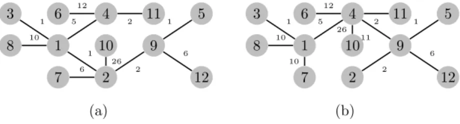
of at least d, or it is a leaf node (a node with degree one). The solution tree is called feasible or admissible and the same designation represent each one of its nodes. Examples of feasible and unfeasible md-MST trees are given in Figures 1 for the graph G1 defined in Appendix A.
8 7 1 3 2 10 4 6 11 12 9 5 1 1 1 2 2 5 6 6 10 12 26 8 7 1 3 2 10 4 6 11 12 9 5 1 1 2 2 5 6 10 10 11 12 26 (a) (b)
Figure 1: Examples of md–MST problem with d = 4, i.e., a m4-MST problem for a given graph G1(see Appendix A). (a) Unfeasible tree ; (b) Feasible tree.
The md-MST problem was first described by Almeida et al. [1] and it was proved to be an NP-hard problem for bn/2c > d ≥ 3 [1, 2]. In order to over-come some of the computational difficulties encountered, Martins and Souza [3] designed new algorithmic approaches based on variable neighbourhood search (VNS) metaheuristics transformed for the md-MST and an enhanced version of a second order repetitive technique (ESO) to guide the search during several phases of the VNS method. They also presented an adaptation of a greedy heuristic based on Kruskal’s algorithm for determining minimal spanning trees.
1 As usual, the final cost is given byP
e∈V ce and a tree with the minimal cost is known
Akg¨un and Tansel [4] considered a new set of degree-enforcing constraints and used the Miller–Tucker–Zemlin sub-tour elimination constraints as an alterna-tive to single or multi-commodity flow constraints for the tree-defining part of the md–MST formulations. Martinez and Cunha [5] proposed new formulations for the md-MST problem and presented a branch-and-cut algorithm based on the original directed formulation, obtainning several new optimality certificates and new best upper bounds for the md-MST. Murthy and Singh [6, 7] pub-lished the only other known evolutionary approach by introducing Artificial Bee Colony and Ant Colony Optimisation heuristics, both tested using Euclidean and random instances for use with Steiner Tree problem instances.
The md-MST requires the computation of a MST with nodes that obey cer-tain degree restrictions. The classical algorithms to construct minimal spanning trees are Prim’s algorithm and Kruskal’s algorithm (KA). Prim’s algorithm [8] starts with a two node tree that contains a minimal edge, and employs a greedy search to build the tree, ensuring that an acyclic tree is obtained. Using a heap as the underlying data structure, this algorithm has a total time bound of O(m + n lg n), where m is the set of edges and n is the set of nodes. KA [9, 10] also uses a greedy technique but works with forests. Starting with the forest of all the nodes, the algorithm iteratively chooses the cheapest edge to join two disjoint nodes until it obtains the complete tree. This algorithm has an asymp-totic time bound of O(m log n) (assuming that the list of edges is already sorted by cost). The MST algorithm used in our approach is the KA. The rationale behind this choice is due mainly to its good numerical performance with generic dense graphs [11] but also because it can be modified easily for our algorithms. Due to the NP-hardness of the problem, an exact algorithm is not usable because of the inherent memory limitations. Thus, a genetic algorithm heuristic is presented, exploring new codings for the candidate spanning trees and opera-tors. The remainder of this paper is organised as follows. Next section begins by summarising the method of Martins and Souza[3] for obtaining feasible spanning trees for the md-MST, in order to explain the original computational improve-ment - MSHOI - of the previous heuristic for generating feasible md-MST trees.
In Section 3, a genetic-based approach to the md-MST problem is introduced, with formulations of three different GA versions. Section 4 reports the results of several computational experiments and the relative efficiency of the different heuristics is discussed. Finally, Section 5 presents concluding remarks as well as suggestions for possible directions for future research.
2. Improvement of the existing heuristic approach to the md-MST 2.1. MSH
Martins and Souza [3] presented a heuristic algorithm (MSH), which uses a modification of Kruskal’s algorithm to build a MST, thereby ensuring the feasibility of the spanning tree but without ensuring its optimality. It is based on evaluating the need values in each step of the KA, i.e., the number of edges that need to be “added” to unfeasible nodes: the nodes i where degT(i) < d.
The total number of edges in a spanning tree is n − 1. If a given candidate tree in the forest (F ) built by KA has k edges, then n − 1 − k edges are still needed to obtain the spanning tree. An edge can be included in a tree only if the need value is less than 2(n − 1 − k) after edge inclusion; otherwise, it is not necessary to consider this edge ever again [3]. Thus, in every intermediate step, MSH computes the overall need value for a forest: total need(F ) = X
∀T ∈F
need(T ), where need(T ) = P
∀i :1<degT(i)<d1. After each KA iteration, the total need
value of the forest and the individual tree need values are re-evaluated until termination by obtaining a complete feasible tree. For each T1, T2∈ F that are
required to be joined, the new tree topology depends on the number of nodes in the tree T1:
1. Size one tree (single node and zero edges): need(T1) = 1. After the
connecting edge has been added, the new tree T has this node as a leaf node, so it is admissible for T .
2. Size two tree (two nodes and one edge): need(T1) = d − 1. For the new
tree T , at least one of the two connecting nodes in T1 or T2 becomes an
3. Other cases: need(T1) = X
∀i :1<degT(i)<d
d − degT(i) if sum not null
1 otherwise
If the sum is null and this is not the final tree, it is necessary to add one edge to connect with another.
2.2. MSHOI - Computatinal improvement of the MSH
As described previously, the MSH’s requirement to compute all of the need tree values at each iteration fundamentally determines the complexity of the algorithm. However, the overall efficiency can be improved by modifying the algorithm so it evaluates only each new need value iteratively based on the previous values. We refer to this improvement as the MSHOI heuristic.
It should be noted that at each step k of the MSH, a pair of trees in the forest Fk, T1and T2, are joined to form a larger tree T . Therefore, the new total
need of the forest can be evaluated only by using the knowledge of T1 and T2
(which are removed from the forest) and the new tree T . Since now we also use the another tree T2besides the T1, there’s a total of six possible cases (excluding
symmetry) to be considered.
Case 1 + 1: Trees T1 and T2 both have size one. Tree T will have two nodes of
degree 1 and one edge, and thus need(T ) = d − 1. The new forest Fk+1 has a
total need of:
total need(Fk+1) = total need(Fk) − 2 + (d − 1) = total need(Fk) + d − 3 .
Case 1 + 2 and Case 2 + 1: Assume that T1 has size one and that T2has size
two, and need = d − 1. Then, need(T ) = d − 2 since T will have one degree 2 node, and thus it is unfeasible.
T1 need(T1) = 1 T2 n1 need(T2) = d − 1 T n1 need(T ) = d − 2
The total need changes to
total need(Fk+1) = total need(Fk) − 1 − (d − 1) + (d − 2) = total need(Fk) − 2 .
Case 2 + 2: Trees T1 and T2 both have size two. Then, two of the nodes of T
will have degree 2, and need(T ) = 2(d − 2). Thus,
total need(Fk+1) = total need(Fk) − 2(d − 1) + 2(d − 2) = total need(Fk) − 2 .
The last two cases imply exactly the same change in the total need so they can be aggregated. All of the previous cases yield a new tree T with unfeasible nodes.
The resulting tree may become feasible when we combine a tree with size three or more with another. This is a special case, so a new variable is intro-duced, inadmTi, to represent the sum of needs for the nodes of a tree Ti. After
joining T1 with T2, if the number of needs for T is zero but it is not a complete
tree (has less than |V | nodes), then the need of T will be 1; otherwise, it will be equal to new inadm, where new inadm is calculated in the following way. Case 1 + 3 and 3 + 1: Consider T1 of size one joining T2 of size 3 or greater.
Then, need(T ) = need(T2). However, three different situations may occur
de-pending on the node n1 of T2used for joining:
1. If degT2(n1) = 1, then it becomes an unfeasible node by increasing its
degree and the new unfeasibility is new inadm = inadmT2+ d − 2;
T1 T2 n1 need(T2) = 0 T n1 need(T ) = d − 2
2. In the case where the degree of n1is less than d, the general unfeasibility
T1 T2 n1 degT2(n1) < d T n1 degT2(n1) increased by 1
3. If the degree of n1 is greater than or equal to d, the unfeasibility value
does not change: new inadm = inadmT2.
T1 T2 n1 degT2(n1) ≥ d T n1 degT(n1) > d
Case 2 + 3 and 3 + 2: Consider tree T1 of size 2 and need = d − 1, which
is joined with a (bigger) tree T2. The degree of the node in T used for the
connection increases by 2, so it will contribute with d−2 to the new unfeasibility. Again, the node n1 to which T1 will be connected influences the feasibility of
the new joint tree.
1. If n1 had degree 1, the new unfeasibility is new inadm = inadmT2+ 2 ×
(d − 2).
2. If the degree is less than d, the unfeasibility is reduced by 1 and increased by d − 2 or new inadm = inadmT2+ d − 3.
3. If the degree was greater than or equal to d, the node is already feasible and so the change in unfeasibility is increased by d − 2 compared with joining with T1, i.e., new inadm = inadmT2+ d − 2.
Case 3 + 3: Two trees of size greater than 2 are joined. In this case, the sum of needs will be calculated separately for each. For T1 and depending on the
node n1 to which T2 is connected, we have the same possibilities described
in (4) when changing inadmT2 for inadmT1. The new unfeasibility for T2,
new inadmT2, is calculated in a similar manner and for the new tree T , we
Determining the new total need (after joining trees T1 and T2) employs the
same iterative procedure,
total need = total need − need(T1) − need(T2) + need(T ) , (1)
thereby proving the following new result.
Theorem 1. For each iteration of the MSH algorithm where 2 sub-trees, T1
and T2, are joined into a new tree T , the new total need is equal to subtracting
the previous total need value of the associated needs for T1 and T2plus the need
of the new tree T .
This implementation results in a few code decision instructions, which are in-dependent of the size of the graph being processed. Consequently, this improve-ment does not require additional usage of resources and the general algorithmic complexity remains the same as that of the original MSH algorithm.
The genetic algorithm approach needs to insure that feasible trees are gene-rated for a successful evolution phase. Therefore, in the following, the improved MSHOI method is used for spanning tree construction.
3. GAs for the md–MST
The proposed approach relies on genetic algorithm (GA) metaheuristics, which are used to investigate a large number of different types of optimisation problems. This class of algorithms is inspired by the Darwinian process of evolution by natural selection [12, 13]. A GA aims to mimic the evolutionary process of species by starting with an initial population of randomly generated candidate solutions, where each individual is represented by a chromosome (its genotype) and each step (or iteration) involves the evolution of the population of candidates guided by a fitness function. This type of heuristic approach is used in the combinatorial optimisation of NP-hard problems [14], where the fitness function is usually referred to as the cost function. The evaluation of the cost function is performed based on the phenotypes, i.e., the individual chromosomes in the population, which is also known as the search space.
The same basic evolutionary strategy is used for all of the genetic variants described in the following, i.e., the classical GA using a predefined number of generations as the stopping criterion.
Algorithm 1 Genetic Algorithm
Initial population random generated using the MSHOI; Sort individuals based on their fitness value;
Choose K with the best fitness as the first evolutionary population; repeat
Select the parental mating pool for reproduction (M P );
Crossover: use the M P to choose two parents for reproduction to obtain a child;
Mutation: decide on the gene mutation for each child;
Selection: select individuals to form the next evolutionary population. until termination criterion is satisfied.
In this genetic approach, selection is mostly elitist. Thus, the selection mechanism retains 50% of the elements with the greatest fitness from the previ-ous evolutionary population and replaces the least fit 50% with the best children of the new offspring. The general reproductive plan of the evolutionary algo-rithm, i.e, the evolution strategy after crossover is the (µ + µ)-ES [15].
Chromosome mutations are controlled by a random function where there is only a low probability of a mutation occurring.
3.1. Fitness function
To evaluate the fitness of a tree, the most obvious choice would be a linear combination of the cost of the tree T and a measurement of its unfeasibility as a penalty function. The latter can be defined by adding the difference between any unfeasible node’s degree and the desired value d, cna(T ). For each candidate
tree T , both costs would then be combined to obtain a fitness function by using the parameter α in a convex combination: αP
α can be set at 0.9 and decreased gradually, thereby forcing infeasible solutions to be rejected increasingly. However, intensive computational tests have shown that the GA versions using this fitness function seldom find admissible trees for values of d above 8 or 9. In order to obtain an effective GA approach, we decided to use the MSHOI heuristic (Section 2.2) so that admissible tree candidate solutions (chromosomes) are always build. Therefore, the fitness function needs no penalty evaluation and is simply taken as the total edge cost of the tree,
F (T ) = X
e∈ET
ce
3.2. Chromosome representations and operators
Based on a thorough investigation of previous studies, we only found two suitable chromosome representations for trees. The first proposes the use of Pr¨ufer numbers, where according to the constructive demonstration of Cay-ley’s formula discovered by Pr¨ufer [16], every such number represents a different spanning tree. Nevertheless, despite its general use, it was argued [17] that this is a poor choice for the implementation of GAs because small changes in the chromosome might cause large differences in the corresponding spanning tree. The second was suggested by Raidl and Julstrom[18] who used a completely dif-ferent representation based on the vector of node weights introduced by Palmer and Kershenbaum [19]. In the following, we describe three different encodings of candidate spanning tree structures with two original representations.
3.2.1. Version gen0 - Using node weights
The authors of [18] suggest the use of a vector based on the weights of the nodes since it can influence the performance of Kruskal’s algorithm. The vector is initialised randomly with weights wi, ∀i ∈ V . When MSHOI is used to
generate a feasible tree, the wiand wjvalues of each of the edge’s {i, j} extreme
nodes will be temporarily added to the current costs of the edge weights: c0ij = cij+ wi+ wj.
To improve efficiency, the edges must be kept in an ordered list. The edges then need to be re-sorted for each candidate solution. A bucket sort2 linear sorting algorithm is used due to the unusual number of orderings required and because the range of the weights of the edges (known a priori) is limited.
For each generation, the reproduction operator alternates between uniform crossover, where each weight is copied randomly either from the father or the mother, and blending with extrapolation. In the latter process, the weight wchild of the new chromosome (child) is obtained by the linear combination of
the parents’ weights as: wchild= β ∗ wdad+ (1 − β) ∗ wmom, −0.5 ≤ β < 1.5.
Next, each element of the chromosome can be mutated according to a given mutation probability parameter by the addition or subtraction of a random amount relative to the respective weight.
3.2.2. Version gen1 - Using the leaf set
A different chromosome representation involves using a set of randomly se-lected leaves. In this case, an array of bits is used to represent the edges in the set. For this version, we need to modify KA in order to avoid choosing edges whose leaves are already joined in the tree. However, not using these might prevent the construction of a spanning tree for non-complete graphs. To over-come this problem, the algorithm goes through the edges again, but without excluding any this time. This phase is never used in a complete graph because all of the leaf nodes are connected to central nodes.
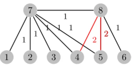
In general, it should be noted that this representation will not guarantee the depiction of all the possible existing trees. For instance, if we consider a graph with eight nodes where the first six are leaves (Figure 2), we need to find a tree with the minimum internal vertex degree d = 3. KA is a greedy strategy, so it always chooses the edges with lower costs to connect leaves to internal nodes, but this will generate a non-admissible solution for the m3-MST problem. For the graph G2, KA will build a tree where five of the leaves are connected to one
1 2 3 4 5 6 7 8 1 1 1 1 1 2 1 1 2 2
Figure 2: Example: Graph G2
internal node of the tree and the remaining internal nodes will be connected with only one leaf, and thus it has an unfeasible degree of 2. However, all of the solutions generated are admissible trees because we use the MSHOI to build the trees.
The gen1 version uses uniform crossover, where each bit is copied at random either from the father or the mother. Before adding the child to the population, mutations are applied with a low probability by flipping bits in the chromosome.
3.2.3. Version gen2 - Using the Edge set
This version represents the chromosome by storing the set of edges in the tree as an array of bits.
When we generate a random set, the probability of hitting a spanning tree is low. In fact, for a complete graph with n nodes and m edges, there are 2m= 2n2−n/2 possible sets of edges. However, only n(n−2) are spanning trees.
For instance, in a complete graph with 25 nodes, only 2523out of 2300 possible sets represent a spanning tree (only one out of 1.43E + 58). Again, KA is employed to overcome this drawback. When a randomly generated set that does not represent a spanning tree, a second phase occurs where KA is repeated but considering all of the edges this time. Unlike the previous version, even for complete graphs this version generally needs to use the second phase to complete the tree.
For gen2 version, reproduction and mutation are alternated between genera-tions. Uniform crossover is used for each even generation, whereas for the odd generations, every individual in the population except the best is subjected to
mutations with a low probability. The mutations are implemented by flipping bits in the chromosome.
4. Computational tests
For comparison with the works of Martinez and Cunha [5] and Martins and Souza [3], the experiments were performed using exactly the same instances as the test-bed. In particular, the three classes of instances, CRD, SYM, and ALM classes, are classic benchmark instances for testing the performance of algorithms for the degree-constrained problem [e.g. 21, 22]. For the weights of the edges, the CRD class uses the Euclidean distance between n randomly generated points within a square. The instances used have 30, 50, 70, and 100 nodes. The SYM class can be defined in a similar manner, except the points are generated in a Euclidean space with higher dimension. In this study, we used 30, 50, and 70 nodes. The ALM class represents larger dimension problems with 100, 200, 300, 400, and 500 nodes. These nodes are evenly distributed points in a grid measuring 480 × 640 and the weights of the edges are the truncated Euclidean distances between the points.
Murthy and Singh [7] use different test sets, namely Euclidean instances for Euclidean Steiner tree problem available from http://people.brunel.ac.uk/ ~mastjjb/jeb/info.html. These consist of randomly distributed points in a unit square considered as nodes of a complete graph, whose edge weights are the Euclidean distances among them.
The minimum bound on the node degree restriction d used as a control parameter depends on the size and of the instances, with values ranging from 3 to 20. All the graphs were complete, and thus m = n2− n.
4.1. Parameters: study and evaluation
The behavior of any GA is affected by various parameters associated with the genetic operators. Those with major effects on the performance comprise the population size (both the original and evolved population sizes), number of
generations, and mutation rate. The first two parameters are crucial because their product is an important measure of the computational efficiency of a GA, and factors such as genetic diversity can be obtained using specifically devised strategies for the crossover and mutation operators. The optimal values are unknown for the md-MST, so we must rely entirely on empirical tests3. After
trial-and-error experiments, it was clear that the best mutation rate value was 3% (although the difference was not significant for 1% or 2%), which agreed with previous studies.
We studied the number of generations and population sizes and their rela-tionship. However, the major difficulty involved is that the algorithm is not deterministic, so the results obtained from each run depend on the pseudo-random generator employed. To determine whether changing a parameter is beneficial for the GA, a statistical criterion must be used to infer the actual significance of differences in performance. We considered two random variables, X1and X2, to represent the costs of the spanning trees obtained after executing
the two versions of the algorithm compared. Given two samples of each, n1and
n2, with dimensions greater than430, where ¯X1, ¯X2and the corrected standard
deviations are ˆS1 and ˆS2, respectively:
| ¯X1− ¯X2| − 1, 65 s ˆ S2 1 n1 + ˆ S2 2 n2 . (2)
If (2) returns a negative value, the difference between the two means is not statistically significant at a level of significance equal to 5% [24].
After several experiments based on evaluations using the significance crite-rion (2), we decided to generate an initial random population twice the size of the evolutionary population. It should be noted that the number of gener-ations required to obtain the best average value did not vary significantly as the population size increased. Although this increase continually improved the
3Another possibility, which we did not explore, is to use online or offline automatic
para-meter tuning methods such as the F-Race method (see [23]).
4Note that 30 represents the theoretical value above which the validity of the test is proved
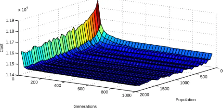
quality of the results, only slight changes occur when the population exceeds a thousand (Figure 3). The improvement was no longer significant so the number
0 200 400 600 800 1000 0 500 1000 1500 2000 1.14 1.15 1.16 1.17 1.18 1.19 x 10⁴ Population Generations Cost
Figure 3: CRD70-2, a 70-node graph instance using d = 10.
of generations required to obtain the best result did not vary greatly with the size of the evolutionary population.
Unlike the size of the evolutionary population, the initial population dimen-sion did not have any significant effects on the final values obtained.
4.2. Comparisons of algorithms’ performance
To evaluate the true effectiveness of the various versions of the GAs, their results were compared with the best published previously. Complete comparison tables can be found in Appendices B and C. The genetic algorithm results are compared with results presented by the authors using the same benchmark graph instances (CRD, SYM and ALM), namely Martinez and Cunha (BC) [5] and Martins and Souza (VNS) [3]. Albeit not sharing the same benchmark instance set, GA results are also compared with the ones reported by Murthy and Singh [7], being at the moment the only other known evolutionary approach.
Akg¨un and Tansel ([4]) also presented comparative results for their meth-ods over some the benchmark instances. However, having only used some of the smaller instances that only improved the run times previously reported by Almeida et al.[1], the results are not effective for use this comparison. More-over, this potential partial advantage is lost when compared with the fastest
results included in [5]. Thus, we will not include Akg¨un and Tansel results in our analysis.
Table 1: Summary of the performance comparisons: GA approach versus Martins-Souza’s final results (VNS) and Martinez-Cunha (BC).
Genetic x VNS Genetic x BC Problems #Instances Better Equal Worse Better Equal Worse CRD 30-100 30 14 14 2 4 23 3
SYM 30-70 24 9 15 - - 19 5
ALM 100-500 36 36 - - 23 2 11
Total 90 59 29 2 27 44 19
4.2.1. Genetic versions versus other heuristics
On most occasions, some version of the GA obtained better (or at least equal) results than the best produced by the VNS heuristics of Martins and Souza [3]. The summary in Table 1 shows that the GA approach obtained better values in 66% of the tests and in only two cases with worse results. The BC heuristics of Martinez and Cunha [5] achieved generally lower values than the previous VNS in terms of the final lower bounds obtained, but the new GA versions are still competitive. In fact, comparing only with BC results, although the percentage of better solutions declined to 30%, the GA approach obtained exactly the same values for 70% of the remaining instances, and presented higher values on only 19 occasions.
In the tables in Appendix B, it is shown that the best value found by the genetic versions has better than all of the best VNS values, with only two exceptions: CRD-2 and CRD-3 using d = 5 (Appendix B, Table 7). The GA strategy is always better than VNS with the hardest instances, the ALM class (Appendix B, Table 7). In terms of the gap values, VNS−VNSmin GA, the genetic algorithms achieved an average value of 8, 17% over all ALM results. In fact, the differences between the final GA values and VNS approaches were significant in terms of the new lower values obtained by GA (Appendix B). Over all test set
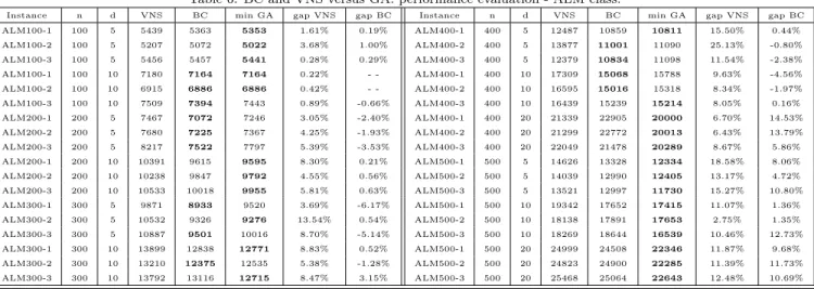
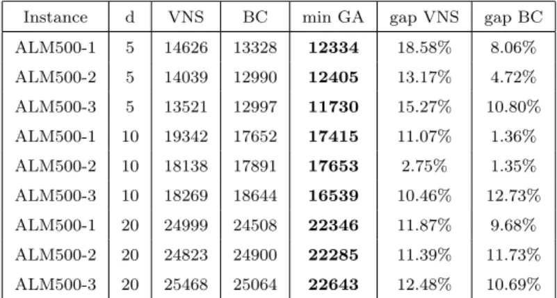
Table 2: BC and VNS best values versus minimum GA versions value performance evaluation - ALM 500 nodes instances.
Instance d VNS BC min GA gap VNS gap BC ALM500-1 5 14626 13328 12334 18.58% 8.06% ALM500-2 5 14039 12990 12405 13.17% 4.72% ALM500-3 5 13521 12997 11730 15.27% 10.80% ALM500-1 10 19342 17652 17415 11.07% 1.36% ALM500-2 10 18138 17891 17653 2.75% 1.35% ALM500-3 10 18269 18644 16539 10.46% 12.73% ALM500-1 20 24999 24508 22346 11.87% 9.68% ALM500-2 20 24823 24900 22285 11.39% 11.73% ALM500-3 20 25468 25064 22643 12.48% 10.69%
instances, the average gap for VNS versus best GA value is 5, 59%.
Comparing only BC and GA results, for the hardest ALM class the average gap value for the better GA results is 4, 52% as detailed in Appendix B. Table 1 shows that 27 new lower bounds were established. It should be noticed that the new GA’s lower values are particularly relevant for the hardest of the instances, the 500 nodes ALM instances (Table 2).
Overall, for the benchmark test set, the GA strategy presents itself as an effective heuristic approach for the md-MST problem, and the more so over the hardest of the instances of the set.
In relation with the works of Murthy and Singh [7], Table 3 is self-explanatory: for the hardest of the fixed Euclidean instances used by these authors, both gen1
and gen2 always perform better. The genetic version gen0 was not tested since
is was designed to work specifically with integer weights and these instances use reals. The GA versions achieved an average gap of 11, 5% and 10, 5% better performance than ABC and ACO heuristics, respectively (AppendixB, Table 5).
Table 3: GA versus ACO and ABC ([7]) for the hardest Euclidean Instances (best and average results for each instance).
ABC ACO gen1 gen2
Name d Best Avg. Best Avg. Best Avg. Best Avg. E250.1 3 15.92 16.08 15.59 15.70 13.077 13.243 12.456 12.762 E250.2 3 15.65 15.85 15.35 15.57 12.852 13.015 12.603 12.865 E250.3 3 15.56 15.72 15.39 15.48 12.854 12.973 12.428 12.760 E250.4 3 15.95 16.09 15.72 15.91 12.788 13.046 12.860 13.021 E250.5 3 15.82 15.95 15.49 15.64 12.895 13.065 12.746 12.888 E250.1 5 19.22 19.59 18.54 19.05 16.454 16.672 16.658 17.254 E250.2 5 19.05 19.29 18.69 19.03 15.552 15.836 16.047 16.355 E250.3 5 18.29 19.10 18.54 18.74 17.087 17.375 15.364 15.735 E250.4 5 19.20 19.73 19.10 19.37 15.940 16.342 16.227 16.642 E250.5 5 18.77 19.23 18.81 19.03 15.882 16.081 16.220 16.449 E250.1 10 24.05 25.23 24.11 24.66 23.359 23.827 23.812 24.222 E250.2 10 24.81 25.49 24.91 25.16 22.303 22.674 22.656 24.094 E250.3 10 24.13 24.88 23.87 24.20 21.755 22.210 22.413 22.933 E250.4 10 25.08 25.69 24.36 25.11 22.745 24.309 23.172 24.016 E250.5 10 24.14 25.06 24.57 25.02 22.494 23.485 23.272 23.682
4.2.2. Run times for the GA versions
This section presents an analysis of the time performance of the GA. The reported times are average run times over 64 runs for each of the GA versions, evolving over 3000 generations with a population size of 3000.
The computer used has an Intel Q9550 processor (Core2 2.83 GHz quadruple core) and 4 GB RAM, so slightly slower than the systems used in the works used for comparison [3, 5, 7]. The RAM capacity was of no consequence because the instance’s dimensions were rather small and we never needed to use more than a small amount of the overall capacity. Therefore, the results of the performance test are directly comparable with those presented in previous studies.
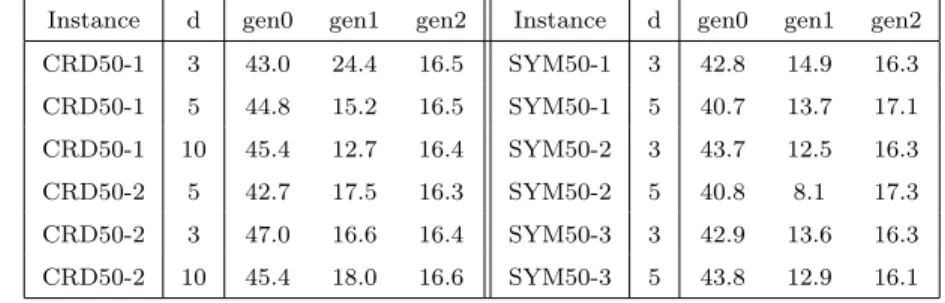
The running times of the GA versions performance is quite stable for any instance and any number of nodes (Appendix C) when compared to the run times presented by Martins and Souza and Martinez and Cunha [3, 5]. Table 4
Table 4: Run times (seconds) for the genetic versions on CRD and SYM instances (graphs with n = 50 nodes).
Instance d gen0 gen1 gen2 Instance d gen0 gen1 gen2 CRD50-1 3 43.0 24.4 16.5 SYM50-1 3 42.8 14.9 16.3 CRD50-1 5 44.8 15.2 16.5 SYM50-1 5 40.7 13.7 17.1 CRD50-1 10 45.4 12.7 16.4 SYM50-2 3 43.7 12.5 16.3 CRD50-2 5 42.7 17.5 16.3 SYM50-2 5 40.8 8.1 17.3 CRD50-2 3 47.0 16.6 16.4 SYM50-3 3 42.9 13.6 16.3 CRD50-2 10 45.4 18.0 16.6 SYM50-3 5 43.8 12.9 16.1
helps the visualisation of the stability of the time performance for the genetic approach, and the same behaviour was observed in all of the CRD, SYM, and ALM classes. Note that gen0 was the slowest of the three versions. In general, for n ≤ 100, gen2 requires less than half the time needed by gen0 and gen1 is slightly faster than gen2, with only a few exceptions. Excluding gen0, the genetic versions are not affected by the different classes of instances and there is no direct relationship between the run time and increasing d.
100 200 300 400 500 Number of nodes 0 1000 2000 3000 4000 5000 6000 Time (seconds) gen0 D=10 gen1 D=10 gen2 D=10 Running times Population 3000, Generations 3000
Figure 4: Comparison of the average run times for the GAs over the ALM class instances using d = 10 for increasing number of nodes.
for any of the genetic versions (Figure 4), which proves that the number of nodes has impact on the run times while maintaining the relative time performance of the three GA versions. Complete graphs were always used so m = O(n2) and the results presented are the worst case example. This explains the higher times required by gen0 because it re-sorts the list of edge weights for each candidate solution (the Bucket Sort algorithm is linear according to the number of edges sorted).
4.2.3. Run times: comparisons with other results
The run times of the GAs depend on the size of the population, the number of generations, and the number of tests for each instance. When these were kept constant, we have shown that the run times were also a function of the number of nodes n.
Martins and Souza [3] present run times that vary greatly, which is particu-larly obvious for the smaller instances. For example, for CRD with n ∈ {30, 50}, VNS requires times that range from only a few seconds to almost 12 minutes. For the same class but with n ∈ {70, 100}, the time ranges from less than 5 minutes to almost 2 hours. For the ALM class, the reported times range from a few thousand to several thousand seconds. These run times do not follow clear patterns of variation relative to the instance dimension or parameters, so it is not possible to directly compare the time required by both approaches. For instance, in the case of ALM300-1 using d = 10, Martins and Souza obtained the best solution with a value of 13899 using almost 4 hours. By contrast, the best result found by the GAs with a smaller cost value of 13701 takes about 23 minutes.
Martinez and Cunha report shorter run times for BC [5] with the simplest of the instances in the test data set, but GA performed better for the all remaining instances, i.e., medium to large size and denser graphs (Appendix C). Especially for the larger and harder of the ALM instances class, GA always outperforms BC both in quality as in time, where BC achieves the maximum tolerate iter-ation time set by the authors. In short, the new GAs generally obtain quality
competitive results in much shorter run times compared with both the VNS and the BC heuristics.
In relation with the evolutionary approach of Murthy and Singh, namely the ABC and ACO heuristics, the GA versions average times for the parameters used are always worse than the former: the best averaged times of the GA is around 6, 5% worst then the ABC, and around 3% worst than the ACO averaged times (Appendix C, Table 10). Nevertheless, the quality of the GA results is much better (Table 3).
5. Conclusions
In this study, we proposed a new algorithmic approach for the approxima-tion of the NP-hard md-MST problem presenting three novel genetic algorithm approaches. An improvement for an existing heuristic procedure for the ob-tention of feasible md-MST trees (MSHOI) was also described. The results obtained with the new algorithms are quite promising, with computationally consistent run times as the instance dimension increases, unlike previously pub-lished direct benchmarking approaches. For these benchmarks, the GA versions achieved lower cost values for over 30% of the instances with competitive and consistent run times. In particular, for the higher instances dimensions, 27 new lower bounds were found, thereby demonstrating that the GA versions provide effective and time efficient solutions to the md-MST problem. Furthermore, when compared with the other known evolutionary approach, using an Artifi-cial Bee Colony and a Ant Colony Optimization heuristics, although more time consuming, the quality of the present GA approach is far superior.
However, some questions remain for future research. First, as usual, the GAs could be made more efficient by enforcing greater genetic diversity in the popu-lation throughout the evolutionary phase. This could be achieved by measuring the difference between each solution and the best obtained to date and using this difference to favour more diverse solutions. Naturally, it is difficult to design a difference function that is both useful and fast. Second, on several occasions, we
found that an optimal parameter or strategy could not be selected because the performance depended on the instance of the problem tested. It might be inter-esting to implement an approach that runs diverse genetic strategies with the option of dynamically adjusting the genetic operators and parameters. Finally, we would like to perform exhaustive testing of this novel GA approach using a more comprehensive data set, ranging from smaller to harder larger dimensional instances and including non Euclidean ones, to facilitate a better evaluation of its empirical computational efficiency.
References
[1] A. M. de Almeida, P. Martins, M. C. de Souza, Min-degree constrained minimum spanning tree problem: complexity, properties, and formulations, International Transactions in Operational Research 19 (3) (2012) 323–352. [2] A. de Almeida, P. Martins, M. C. de Souza, The md-mst problem is np-hard
for d ≥ 3, Electronic Notes for Discrete Mathematics 36 (2010) 9–15. [3] P. Martins, M. C. de Souza, Vns and second order heuristics for the
min-degree constrained minimum spanning tree problem, Computers & Opera-tions Research 36 (11) (2009) 2969–2982.
[4] B. Akg¨un, I.and Tansel, Min-degree constrained minimum spanning tree problem: New formulation via miller-tucker-zemlin constraints, Computers & Operations Research 37 (1) (2010) 72–82.
[5] L. C. Martinez, A. Cunha, The min-degree constrained minimum span-ning tree problem: Formulations and branch-and-cut algorithm, Discrete Applied Mathematics (164) (2014) 210–224.
[6] V. V. R. Murthy, A. Singh, Solving the min-degree constrained minimum spanning tree problem using heuristic and metaheuristic approaches, in: Proc. of the Second IEEE International Conference on Parallel, Distributed and Grid Computing (PDGC 2012), IEEE Press, 2012, pp. 716–720.
[7] V. V. R. Murthy, A. Singh, An ant colony optimization algorithm for the min-degree constrained minimum spanning tree problem, in: B. Panigrahi, P. Suganthan, S. Das, S. Dash (Eds.), Swarm, Evolutionary, and Memetic Computing, Vol. 8298 of Lecture Notes in Computer Science, Springer In-ternational Publishing, 2013, pp. 85–94.
[8] R. C. Prim, Shortest connection networks and some generalizations, Bell System Technical Journal (36) (1957) 1389–1401.
[9] J. B. Kruskal, On the shortest spanning subtree of a graph and the trav-elling salesman problem., in: Proc. of the American Mathematical Society, 1956, pp. 48–50.
[10] M. Gondran, M. Minoux, Graphs and algorithms, John Wiley & Sons, Chichester, UK, 1984.
[11] A. de Almeida, R. Salgueiro, Recovering a labeling algorithm for the disjoint-set problem to improve kruskal’s effciency on dense graphs, tR2015/02, CISUC (February 2015).
[12] R. L. Haupt, S. E. Haupt, Practical genetic algorithms, John Wiley & Sons, Inc., New York, NY, USA, 1998.
[13] Z. Michalewicz, Genetic algorithms + data structures = evolution pro-grams, 2nd Edition, Springer-Verlag New York, Inc., New York, NY, USA, 1994.
[14] C. M. Papadimitriou, Computational complexity, Addison-Wesley, Mas-sachusetts, 1994.
[15] H.-G. Beyer, H.-P. Schwefel, Evolution strategies – a comprehensive intro-duction, Natural Computing 1 (1) (2002) 3–52.
[16] H. Pr¨uffer, Neuer beweis eines satzes ¨uber permutationen, Archiv f¨ur Math-ematik und Physik (1918) 742–744.
[17] J. Gottlieb, B. Julstrom, G. Raidl, F. Rothlauf, Pr¨ufer numbers: A poor representation of spanning trees for evolutionary search, in: L. Spector, E. D. Goodman, A. Wu, W. B. Langdon, H.-M. Voigt, M. Gen, S. Sen, M. Dorigo, S. Pezeshk, M. H. Garzon, E. Burke (Eds.), Proc. of the Ge-netic and Evolutionary Computation Conference (GECCO-2001), Morgan Kaufmann, San Francisco, California, USA, 2001, pp. 343–350.
[18] G. Raidl, B. Julstrom, A weighted coding in a genetic algorithm for the degree-constrained minimum spanning tree problem, in: Proc. in the ACM Symposium in Applied Computing, 2000, pp. 440–445.
[19] C. Palmer, A. Kershenbaum, Representing trees in genetic algorithms, in: Proc. of the First IEEE Conference on Evolutionary Computation, Vol. 1, 1994, pp. 379–384.
[20] T. H. Cormen, C. E. Leiserson, R. L. Rivest, C. Stein, Introduction to Algorithms, 2nd Edition, The MIT Press, 2001.
[21] M. Krishnamoorthy, A. Ernst, Y. Sharaiha, Comparison of algorithms for the degree constrained spanning tree, Journal of Heuristics 7 (2001) 587– 611.
[22] C. Ribeiro, M. de Souza, Variable neighborhood search for the degree con-strained minimum spanning tree problem, Discrete Applied Mathematics 118 (2002) 43–54.
[23] M. Birattari, Tuning Metaheuristics: A Machine Learning Perspective, 1st Edition, Springer, 2009.
[24] S. M. Ross, Introduction to Probability and Statistics for Engineers and Scientists, 3rd Edition, Elsevier Academic Press, 2004.
Appendix A
Let G1= (V, E), where V = {1, 2, 3, . . . , 12} is the graph.
8 7 1 3 2 10 4 6 11 12 9 5 Figure 5: Graph G1.
The associated edge costs are given by the adjacency matrix C, as follows.
C = – 1 1 5 26 – 10 10 – – – 48 1 – 28 – 67 – 6 – 2 26 – – 1 28 – – – 40 – 38 – – 57 – 5 – – – 34 12 – – 11 26 2 – 26 67 – 34 – – 102 – 1 – – – – – 40 12 – – 65 30 – 53 – – 10 6 – – 102 65 – – 110 – – – 10 – 38 – – 30 – – 54 – – 67 – 2 – 11 1 – 110 – – – – 6 – 26 – 26 – 53 54 – – – 45 – – – 57 2 – – – – – 45 – 90 48 – – – – – – 67 6 – 90 – (3)
Appendix B: Genetic Algorithms Strategy Quality Performance Evaluation
Comparison of the minimum of objective function values obtained by the GA approaches (gen0, gen1, and gen2), min GA, with the lower bounds of VNS [3] and BC [5] heuristics, and the best values of ACO and ABC heuristics [7]. Also shown are the gap differences X−min GA
min GA , where min GA stands for the minimum value obtained between the genetic algorithm versions and X is the heuristics value in comparison (VNS, BC, ABC, or ACO).
Table 5: Comparison of gen1 and gen2 with ACO and ABC heuristics [7] for the 250 nodes Euclidean instances.
ABC ACO gen1 gen2 gap ABC gap ACO
Name d Best Avg. Best Avg Best Avg. Best Avg.
E250.1 3 15.92 16.08 15.59 15.70 13.08 13.24 12.46 12.76 27,77% 25,12% E250.2 3 15.65 15.85 15.35 15.57 12.85 13.02 12.61 12.87 24,11% 21,73% E250.3 3 15.56 15.72 15.39 15.48 12.85 12.97 12.43 12.76 25,18% 23,81% E250.4 3 15.95 16.09 15.72 15.91 12.79 13.05 12.86 13.02 24,71% 22,91% E250.5 3 15.82 15.95 15.49 15.64 12.9 13.07 12.75 12.89 24,08% 21,49% E250.1 5 19.22 19.59 18.54 19.05 16.45 16.67 16.66 17.25 16,84% 12,71% E250.2 5 19.05 19.29 18.69 19.03 15.55 15.84 16.05 16.36 22,51% 20,19% E250.3 5 18.29 19.10 18.54 18.74 17.09 17.38 15.36 15.74 19,08% 20,70% E250.4 5 19.20 19.73 19.10 19.37 15.94 16.34 16.23 16.64 20,45% 19,82% E250.5 5 18.77 19.23 18.81 19.03 15.88 16.08 16.22 16.45 18,20% 18,45% E250.1 10 24.05 25.23 24.11 24.66 23.36 23.83 23.81 24.22 2,95% 3,21% E250.2 10 24.81 25.49 24.91 25.16 22.30 22.67 22.66 24.09 11,26% 11,70% E250.3 10 24.13 24.88 23.87 24.20 21.76 22.21 22.413 22.93 10,89% 9,70% E250.4 10 25.08 25.69 24.36 25.11 22.75 24.31 23.17 24.02 10,24% 7,08% E250.5 10 24.14 25.06 24.57 25.02 22.49 23.49 23.27 23.68 7,34% 9,25% 26
Table 6: BC and VNS versus GA: performance evaluation - ALM class.
Instance n d VNS BC min GA gap VNS gap BC Instance n d VNS BC min GA gap VNS gap BC
ALM100-1 100 5 5439 5363 5353 1.61% 0.19% ALM400-1 400 5 12487 10859 10811 15.50% 0.44% ALM100-2 100 5 5207 5072 5022 3.68% 1.00% ALM400-2 400 5 13877 11001 11090 25.13% -0.80% ALM100-3 100 5 5456 5457 5441 0.28% 0.29% ALM400-3 400 5 12379 10834 11098 11.54% -2.38% ALM100-1 100 10 7180 7164 7164 0.22% - - ALM400-1 400 10 17309 15068 15788 9.63% -4.56% ALM100-2 100 10 6915 6886 6886 0.42% - - ALM400-2 400 10 16595 15016 15318 8.34% -1.97% ALM100-3 100 10 7509 7394 7443 0.89% -0.66% ALM400-3 400 10 16439 15239 15214 8.05% 0.16% ALM200-1 200 5 7467 7072 7246 3.05% -2.40% ALM400-1 400 20 21339 22905 20000 6.70% 14.53% ALM200-2 200 5 7680 7225 7367 4.25% -1.93% ALM400-2 400 20 21299 22772 20013 6.43% 13.79% ALM200-3 200 5 8217 7522 7797 5.39% -3.53% ALM400-3 400 20 22049 21478 20289 8.67% 5.86% ALM200-1 200 10 10391 9615 9595 8.30% 0.21% ALM500-1 500 5 14626 13328 12334 18.58% 8.06% ALM200-2 200 10 10238 9847 9792 4.55% 0.56% ALM500-2 500 5 14039 12990 12405 13.17% 4.72% ALM200-3 200 10 10533 10018 9955 5.81% 0.63% ALM500-3 500 5 13521 12997 11730 15.27% 10.80% ALM300-1 300 5 9871 8933 9520 3.69% -6.17% ALM500-1 500 10 19342 17652 17415 11.07% 1.36% ALM300-2 300 5 10532 9326 9276 13.54% 0.54% ALM500-2 500 10 18138 17891 17653 2.75% 1.35% ALM300-3 300 5 10887 9501 10016 8.70% -5.14% ALM500-3 500 10 18269 18644 16539 10.46% 12.73% ALM300-1 300 10 13899 12838 12771 8.83% 0.52% ALM500-1 500 20 24999 24508 22346 11.87% 9.68% ALM300-2 300 10 13210 12375 12535 5.38% -1.28% ALM500-2 500 20 24823 24900 22285 11.39% 11.73% ALM300-3 300 10 13792 13116 12715 8.47% 3.15% ALM500-3 500 20 25468 25064 22643 12.48% 10.69% 27
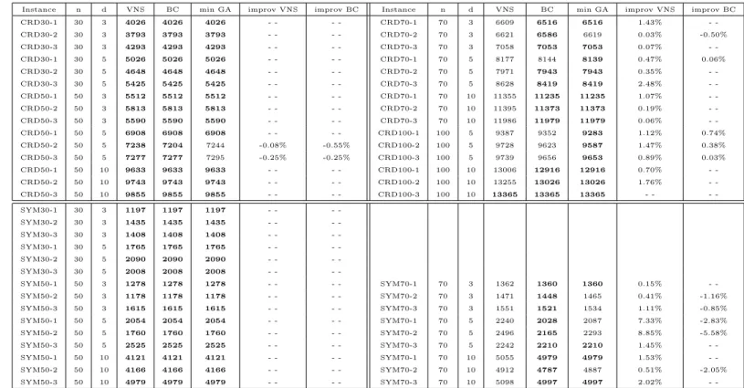
Table 7: BC and VNS versus GA: performance evaluation - CRD and SYM classes.
Instance n d VNS BC min GA improv VNS improv BC Instance n d VNS BC min GA improv VNS improv BC
CRD30-1 30 3 4026 4026 4026 - - - - CRD70-1 70 3 6609 6516 6516 1.43% -CRD30-2 30 3 3793 3793 3793 - - - - CRD70-2 70 3 6621 6586 6619 0.03% -0.50% CRD30-3 30 3 4293 4293 4293 - - - - CRD70-3 70 3 7058 7053 7053 0.07% -CRD30-1 30 5 5026 5026 5026 - - - - CRD70-1 70 5 8177 8144 8139 0.47% 0.06% CRD30-2 30 5 4648 4648 4648 - - - - CRD70-2 70 5 7971 7943 7943 0.35% -CRD30-3 30 5 5425 5425 5425 - - - - CRD70-3 70 5 8628 8419 8419 2.48% -CRD50-1 50 3 5512 5512 5512 - - - - CRD70-1 70 10 11355 11235 11235 1.07% -CRD50-2 50 3 5813 5813 5813 - - - - CRD70-2 70 10 11395 11373 11373 0.19% -CRD50-3 50 3 5590 5590 5590 - - - - CRD70-3 70 10 11986 11979 11979 0.06% -CRD50-1 50 5 6908 6908 6908 - - - - CRD100-1 100 5 9387 9352 9283 1.12% 0.74% CRD50-2 50 5 7238 7204 7244 -0.08% -0.55% CRD100-2 100 5 9728 9623 9587 1.47% 0.38% CRD50-3 50 5 7277 7277 7295 -0.25% -0.25% CRD100-3 100 5 9739 9656 9653 0.89% 0.03% CRD50-1 50 10 9633 9633 9633 - - - - CRD100-1 100 10 13006 12916 12916 0.70% -CRD50-2 50 10 9743 9743 9743 - - - - CRD100-2 100 10 13255 13026 13026 1.76% -CRD50-3 50 10 9855 9855 9855 - - - - CRD100-3 100 10 13365 13365 13365 - - -SYM30-1 30 3 1197 1197 1197 - - -SYM30-2 30 3 1435 1435 1435 - - -SYM30-3 30 3 1408 1408 1408 - - -SYM30-1 30 5 1765 1765 1765 - - -SYM30-2 30 5 2090 2090 2090 - - -SYM30-3 30 5 2008 2008 2008 - - -SYM50-1 50 3 1278 1278 1278 - - - - SYM70-1 70 3 1362 1360 1360 0.15% -SYM50-2 50 3 1178 1178 1178 - - - - SYM70-2 70 3 1471 1448 1465 0.41% -1.16% SYM50-3 50 3 1615 1615 1615 - - - - SYM70-3 70 3 1551 1521 1534 1.11% -0.85% SYM50-1 50 5 2054 2054 2054 - - - - SYM70-1 70 5 2240 2028 2087 7.33% -2.83% SYM50-2 50 5 1760 1760 1760 - - - - SYM70-2 70 5 2496 2165 2293 8.85% -5.58% SYM50-3 50 5 2525 2525 2525 - - - - SYM70-3 70 5 2242 2210 2210 1.45% -SYM50-1 50 10 4121 4121 4121 - - - - SYM70-1 70 10 5055 4979 4979 1.53% -SYM50-2 50 10 4166 4166 4166 - - - - SYM70-2 70 10 4912 4787 4887 0.51% -2.05% SYM50-3 50 10 4979 4979 4979 - - - - SYM70-3 70 10 5098 4997 4997 2.02% -28
Appendix C: Run times for the GA versions
Average performance times based on 64 runs of each test instance for each genetic version: gen0, gen1, and gen2 and the respective BC [5] run times, with the exception of the last table, were the vast majority of run times reported for BC are maximum tolerated iteration times.
Table 8: Average run times (seconds) of the GA versions: CRD and SYM instance graphs (n ≤ 100).
Instance d gen0 gen1 gen2 BC Instance d gen0 gen1 gen2 BC
CRD30-1 3 19.6 13.9 7.3 0.3 SYM30-1 3 19.2 4.7 7.6 0.2 CRD30-1 5 20.5 6.7 7.2 0.9 SYM30-1 5 19.9 5.5 7.4 0.5 CRD30-2 3 19.4 5.6 7.3 0.2 SYM30-2 3 19.1 4.9 7.6 0.1 CRD30-2 5 20.0 8.7 7.2 0.3 SYM30-2 5 20.0 7.2 7.4 0.3 CRD30-3 3 19.3 7.2 7.5 0.2 SYM30-3 3 18.8 4.6 7.8 0.0 CRD30-3 5 20.5 7.2 7.2 3.2 SYM30-3 5 19.5 11.6 7.5 0.1 CRD50-1 3 43.0 24.4 16.5 5.0 SYM50-1 3 42.8 14.9 16.3 0.7 CRD50-1 5 44.8 15.2 16.5 69.0 SYM50-1 5 40.7 13.7 17.1 5.7 CRD50-1 10 45.4 12.7 16.4 13.8 SYM50-2 3 43.7 12.5 16.3 0.7 CRD50-2 5 42.7 17.5 16.3 81.2 SYM50-2 5 40.8 8.1 17.3 1.3 CRD50-2 3 47.0 16.6 16.4 61.6 SYM50-3 3 42.9 13.6 16.3 0.2 CRD50-2 10 45.4 18.0 16.6 7.7 SYM50-3 5 43.8 12.9 16.1 10.9 CRD70-1 3 77.3 33.6 32.5 148.6 SYM70-1 3 70.1 36.6 30.7 1.9 CRD70-1 5 78.1 26.9 30.1 800.0 SYM70-1 5 73.4 18.0 30.1 7.3 CRD70-1 10 78.5 20.7 30.2 138.6 SYM70-1 10 76.6 21.2 30.1 115.9 CRD70-2 3 75.0 23.1 30.4 4785.0 SYM70-2 3 70.9 18.9 30.5 6.0 CRD70-2 5 74.9 23.8 29.8 2416.9 SYM70-2 5 73.4 17.2 30.1 5.0 CRD70-2 10 78.2 28.3 29.9 571.9 SYM70-2 10 75.7 22.6 29.8 53.0 CRD70-3 3 75.7 25.6 30.2 3859.9 SYM70-3 3 72.1 19.5 31.9 4.8 CRD70-3 5 77.1 21.2 29.8 1402.8 SYM70-3 5 73.1 21.8 30.1 31.6 CRD70-3 10 76.6 24.7 30.6 17.9 SYM70-3 10 75.6 21.5 29.7 112.9 CRD100-1 3 137.1 57.5 62.1 - ALM100-1 3 125.5 52.5 60.0 -CRD100-1 5 140.6 47.2 60.5 10800.0 ALM100-1 5 129.5 51.2 59.3 21600.0 CRD100-1 10 131.5 51.9 59.8 5741.6 ALM100-1 10 127.6 56.3 59.4 385.4 CRD100-2 3 129.4 91.3 61.3 - ALM100-2 3 125.7 55.5 62.7 -CRD100-2 5 146.9 68.0 61.2 10800.0 ALM100-2 5 130.8 59.1 63.4 21600.0 CRD100-2 10 133.9 49.7 59.9 669.4 ALM100-2 10 128.4 51.9 59.6 7706.1 CRD100-3 3 137.9 60.9 63.5 - ALM100-3 3 126.9 47.3 60.7 -CRD100-3 5 144.4 63.1 60.5 10800.0 ALM100-3 5 131.8 55.8 60.5 21600.0 CRD100-3 10 134.9 42.1 60.3 1359.4 ALM100-3 10 128.8 58.4 60.5 21600.0
Table 9: Average run times (seconds) of the GA versions: ALM instance graphs (n > 100).
Instance n d gen0 gen1 gen2 Instance n d gen0 gen1 gen2
ALM200-1 200 3 497.0 273.2 261.6 ALM300-1 300 3 1169.3 411.3 566.6 ALM200-1 200 5 527.9 219.3 251.7 ALM300-1 300 5 1193.4 438.5 564.5 ALM200-1 200 10 509.7 201.9 245.9 ALM300-1 300 10 1237.0 474.7 553.5 ALM200-2 200 3 504.9 231.3 268.8 ALM300-2 300 3 1181.5 554.0 619.2 ALM200-2 200 5 523.2 256.2 247.9 ALM300-2 300 5 1185.3 443.2 569.7 ALM200-2 200 10 509.7 182.2 247.0 ALM300-2 300 10 1224.6 445.5 573.0 ALM200-3 200 3 501.6 224.9 257.5 ALM300-3 300 3 1173.6 459.4 605.4 ALM200-3 200 5 518.7 210.2 252.4 ALM300-3 300 5 1195.9 506.0 580.6 ALM200-3 200 10 515.1 231.4 250.5 ALM300-3 300 10 1230.6 480.8 577.1 ALM400-1 400 3 2296.7 864.4 1153.0 ALM400-1 400 5 2503.2 912.3 1044.5 ALM500-1 500 5 5338.9 1652.3 1662.9 ALM400-1 400 10 2498.2 811.4 1028.9 ALM500-1 500 10 5433.9 1260.3 1997.7 ALM400-1 400 20 2526.2 701.6 1285.7 ALM500-1 500 20 5384.2 1302.1 2144.2 ALM400-2 400 3 2321.0 832.0 1035.7 ALM400-2 400 5 2374.0 906.1 1019.1 ALM500-2 500 5 5292.5 1541.0 1692.1 ALM400-2 400 10 2499.0 850.3 1022.1 ALM500-2 500 10 5444.3 1382.3 1854.3 ALM400-2 400 20 2385.2 719.9 1156.5 ALM500-2 500 20 5285.6 1184.3 1928.3 ALM400-3 400 3 2317.9 878.1 1078.5 ALM400-3 400 5 2370.4 1022.7 1030.8 ALM500-3 500 5 5257.6 594.7 1666.5 ALM400-3 400 10 2496.4 819.8 1036.8 ALM500-3 500 10 5376.9 1318.7 1735.7 ALM400-3 400 20 2354.3 787.1 1242.9 ALM500-3 500 20 5320.0 1126.2 1809.3
Table 10: Average run times (seconds) of gen1 and gen2 for the 250 nodes Euclidean instances compared with ABC and ACO heuristics [7]
Name d ABC ACO gen1 gen2 Name d ABC ACO gen1 gen2
E250.1 3 96.81 273.51 874.13 918.83 E250.1 10 96.16 108.78 683.07 1037.82 E250.2 3 89.05 296.32 516.04 871.47 E250.2 10 105.29 107.14 613.44 982.23 E250.3 3 89.52 284.62 681.29 852.30 E250.3 10 108.72 106.63 406.26 984.35 E250.4 3 96.59 286.20 605.41 850.86 E250.4 10 104.29 102.73 710.56 1005.81 E250.5 3 103.74 272.22 817.51 789.27 E250.5 10 104.99 101.73 737.53 985.97 E250.1 5 98.34 195.69 650.40 1013.87 E250.2 5 106.52 203.36 574.67 1013.70 E250.3 5 95.35 191.98 633.26 992.89 E250.4 5 99.53 172.76 691.03 1031.76 E250.5 5 89.88 170.54 506.76 982.03

![Table 3: GA versus ACO and ABC ([7]) for the hardest Euclidean Instances (best and average results for each instance).](https://thumb-eu.123doks.com/thumbv2/123dok_br/19187023.948043/19.918.203.716.251.618/table-versus-hardest-euclidean-instances-average-results-instance.webp)
![Table 5: Comparison of gen1 and gen2 with ACO and ABC heuristics [7] for the 250 nodes Euclidean instances.](https://thumb-eu.123doks.com/thumbv2/123dok_br/19187023.948043/27.1188.325.859.397.633/table-comparison-aco-abc-heuristics-nodes-euclidean-instances.webp)