Equilibrium price dynamics in an
overlapping-generations exchange economy
Paulo Brito
1and Rui Dil˜
ao
2October 31, 2006
1) UECE, Instituto Superior de Economia e Gest˜ao, Technical University of Lisbon, R. Miguel Lupi 20, 1249-078 Lisbon, Portugal.
2) Nonlinear Dynamics Group, Instituto Superior T´ecnico, Technical Uni-versity of Lisbon, Av. Rovisco Pais, 1049-001 Lisbon, Portugal.
[email protected]; [email protected]
Abstract
We present a continuous time overlapping generations model for an endowment Arrow-Debreu economy with an age-structured popu-lation. For an economy with a balanced growth path, we prove that Arrow-Debreu equilibrium prices exist, and their dynamic properties are age-dependent. Our model allows for an explicit dependence of prices on critical age-specific endowment parameters. We show that, if endowments are distributed earlier than some critical age, then spec-ulative bubbles for prices do exist.
Keywords: Arrow-Debreu equilibrium, overlapping generations models, McKendrick model.
1
Introduction
There is a growing evidence that the major impact of demography into econ-omy is more significant when the age-structure of a population is taken into account. For example, the change in mortality and fertility that occurs dur-ing demographic transitions is contemporaneous to the onset of modern eco-nomic growth1. Long run cycles in both productivity2 and asset prices3
dis-play frequencies roughly similar to the ones found in the age-composition of populations. At the microeconomic level, variables such as wage, consump-tion and savings display life-cycle patterns, and, therefore, are also clearly age-dependent4.
Overlapping generations (OLG) models consider economies with several cohorts (Samuelson (1958) and Diamond (1965)). They are general macroe-conomic equilibrium models, where the equilibrium is determined by aggre-gating agents belonging to different cohorts. These models have a source of heterogeneity that is related to differences in the economic behaviour of peo-ple along their life-cycles. This raises difficult conceptual and mathematical questions that are associated with the process of modelling aggregation and with the definition of general equilibrium.
For these reasons, most results in OLG models have been established for the case where the representative households have a two-period lifetime. Several issues have been analysed as, for instance, the existence and Pareto-efficiency of equilibrium and its determinacy, the dynamics of asset prices, the existence of speculative bubbles, and the presence of endogenous fluctuations in the economy. For a survey, see Geanakoplos and Polemarchakis (1991).
In this paper we consider a continuous time OLG model. According to assumptions regarding the lifetime of the representative members of different generations, we divide the existing OLG models into to categories: uncertain lifetime and certain lifetime models.
The macroeconomic equilibrium model of Blanchard (1985) is the sem-inal contribution for the uncertain lifetime strand of models. It assumes a Yaari (1965) annuity market, a production economy, cohort heterogeneity, and a Radner equilibrium. Demographic assumptions are essential in the
1
Galor and Weil (2000).
2
Lindh and Malmberg (1999), Poterba (2001), Azariadis et al. (2004) and Beaudry et al. (2005).
3
Geanakoplos et al. (2004).
4
determination of the probability of survival for the representative consumer. All the numerous extensions usually feature a macroeconomic equilibrium described by ordinary differential equations, implying that the age-structure affects neither aggregate activity nor asset prices. This is a consequence of the particular assumptions regarding demography.
In the general equilibrium model of Cass and Yaari (1967), agents have a finite or infinite certain lifetime. They has been recently extended in several directions by Boucekkine et al. (2002), d’Albis and Augeraud-Veron (2004) and Demichelis and Polemarchakis (2006). In these models it is assumed a representative agent with a fixed lifetime, cohort heterogeneity, and a pop-ulation with exponential growth. As the representative agent behaviour is specified independently of any demographic variables, the assumption of ex-ponential growth implies that equilibrium is independent from demography. In these models, the most common assumption is that consumers have a one-period lifetime, and the general macroeconomic equilibrium is represented by mixed functional differential equations, or, in the case of Demichelis and Polemarchakis (2006), by a convolution type integral equation with a finite interval of integration. In general, solutions depend on the lifetime duration of the representative agent.
In this paper, we consider uncertain lifetime OLG models and we extend them in order to allow for a more realistic, age-dependent, demography and lifetime income distribution. We consider an exchange economy, in which there is a single good, a system of Arrow-Debreu markets and we assume that the representative agent of a cohort has a Yaari-Blanchard uncertain lifetime utility functional5. The population is described by the age-structured
McKendrick (1926) model of demography. As the density of individuals of the population is a weighting factor for the determination of aggregate vari-ables, the age-dependent demographic variables are introduced in a natural way. Demography variables enter both in the specification of the represen-tative consumer behaviour and in the definition of the aggregate equilibrium condition.
As time is continuous, there is an infinite number of markets in which forward transactions for delivery of a single good at every moment in time are performed. In other words, we consider a complete system of Arrow-Debreu prices. For this economy, we show that the equilibrium prices are described by a double integral equation, with both backward and forward
5
intertemporal dependence, and whose solution is independent of the lifetime of the consumers. This equation depends on both economic and demographic age-structured variables. Our setting allows for the study of the effects of age-specific shocks in both endowments and demography on equilibrium asset prices.
In order to obtain exact explicit results, we solve the double integral equation for particular cases where the economy follows balanced growth paths. We consider two cases: A benchmark case, where all the endowments are distributed at a specific age, and a case in which endowments are constant through the life-cycle but cease at a retirement age.
We prove that equilibrium prices exist and may display (rational) specula-tive bubbles. The existence of (rational) speculaspecula-tive bubbles in OLG models has been already documented in the literature (see LeRoy (2004)). Here, we determine analytical conditions for their existence, as a function of the age-distribution of endowments and of the age of retirement. We show that, if endowments are distributed earlier than some critical age, then speculative bubbles for prices do exist.
In the case of time independent and constant endowments up to a re-tirement age, the equilibrium equation for prices derived in this paper is formally similar to the one found in Demichelis and Polemarchakis (2006). In the more general case analysed here, we prove the existence of a critical age separating bounded from unbounded price dynamics.
This paper is organized as follows. In section 2 we summarize the results on the McKendrick model of population dynamics that will be used along this paper. In section 3, we derive the overlapping generations model in continuous time, and we arrive at a double integral equation describing the equilibrium prices of our model. In section 4, we prove that equilibrium prices exist and we characterize their dynamics. In the last section, we discuss the main conclusions of the paper and further directions of research.
2
Demography with an age-structured
popu-lation model
by the function n(a, t). At time t, the total number of individuals in the population is,
N(t) =
+∞
Z
0
n(a, t)da . (1)
The time evolution of the density of individuals of an age-structured popula-tion can be simply described by the first order partial differential equapopula-tion,
dn(a, t)
dt =
∂n(a, t)
∂t +
∂n(a, t)
∂a =−µ(a)n(a, t) (2)
where da
dt = 1, and µ(a) is the age-dependent mortality modulus of the
pop-ulation. As n1dndt = −µ(a), the mortality modulus is the per-capita age-dependent death rate of the population. New-borns are introduced through the boundary condition,
n(0, t) = Z +∞
0 b(a, t)n(a, t)da (3)
where b(a, t) is the fertility function of age class a at time t. Equation (2), together with the boundary condition (3), defines the age-structured McK-endrick model of population growth, McKMcK-endrick (1926). The existence of solutions of the Cauchy problem for the linear equation (2) together with the boundary condition (3) is well established by semigroup techniques and by the method of characteristics. For reviews see, for example, Webb (1985), Cushing (1998) and Dil˜ao (2006).
The population density at timetis determined from the initial population density, n(a, t = 0) = ψ(a), with a, t ∈ R+. According to the standard
theory of first order partial differential equations, the characteristic curves of the McKendrick equation are the solutions of the differential equation da
dt = 1,
being straight lines with equation,a−a0 =t−t0, Dil˜ao (2006). Therefore, as
dn
dt =−µ(a)n, within a characteristic curve, the solutions of the McKendrick
equation can be written as,
n(a, t) =n(a0, t0) exp
−
Z t
t0
µ(s+a0−t0)ds
(4)
For given time independent mortality modulusµ(a) and fertility function
b(a), the time independent solutions of the McKendrick equation obey the ordinary differential equation,
dn¯
da =−µ(a)¯n (5)
with the boundary (initial) condition,
¯
n0 =
Z +∞
0 b(a)¯n(a)da . (6)
The solution of the time independent equation (5) is,
¯
n(a) = ¯n0e
−R
a
0 µ(s)ds. (7)
Multiplying (7) by b(a) and integrating ina, by the boundary condition (6), we obtain,
Z +∞
0 b(a)e
−Ra
0 µ(s)dsda= 1. (8)
Introducing the Lotka growth rate defined by,
r= Z +∞
0 b(a)e
−R
a
0 µ(s)dsda (9)
then, if the McKendrick equation has a non-zero time independent solution, the Lotka growth number is r= 1. In this case, the equilibrium distribution of the population is given by (7).
The exponential term in the definition of Lotka growth rate can be un-derstood as the probability of survival of an individual of the population up to age a,
π(a) = e−R
a
0 µ(s)ds. (10)
For example, choosing a constant mortality modulus µ, the equilibrium solution of the McKendrick equation is ¯n(a) = ¯n0e−µa. In this case, the total
population number is N(t) = ¯n0/µ, and b(a) and ¯n0 obey to the condition,
¯
n0
Z +∞
0 b(a)e
−µada= 1.
3
The OLG model
In order to analyse the general equilibrium behaviour of prices in economies with age-structured populations, we consider an endowment economy6 in
which a single product is exogenously available, it is not storable, and it is only used for consumption. The representative agent has an age-dependent stream of endowments, and determines the optimal lifetime consumption by maximizing an intertemporal utility functional. This intertemporal utility functional has a logarithmic instantaneous utility function. We also assume that there are neither bequests nor intra- or intergenerational transfers. The time flows continuously and the economy is populated by individuals belong-ing to different cohorts. Individuals are considered sbelong-ingle households.
We call cohortt0 to the density of individuals born at timet0. At t=t0,
the density of individuals in the cohort is n(t0) = n(0, t0). Along lifetime,
this density decays proportionally toπ(a), as shown in the previous sections. We assume a complete system of Arrow-Debreu contracts: At the time of birth, consumers make spot transactions and perform forward contracts for delivery of the good at any instant along their lifetimes. As it is well known in OLG economies, we further consider that all the markets open at timet= 0 and the prices set at t= 0 prevail for the contracts performed by future cohorts (Geanakoplos and Polemarchakis (1991)). This institutional framework implies that the decisions of the representative member of every cohort are subject to a static budget constraint at the time of birth7.
3.1
The representative consumer problem
The representative member of the cohortt0 (a= 0) has an uncertain lifetime.
As in Yaari (1965), at the time of birth, the representative member of the cohort chooses a lifetime flow of consumption, c(a, t) = c(a, t0 +a), with
a∈R+, which maximizes the utility functional,
U(t0) =
Z ∞
0 ln(c(a, t0+a))R(a)π(a)da, (11)
6
In the early literature, this case has been analysed in the context of two and three periods lifetime cases. See, for example, Samuelson (1958), Shell (1971), and Balasko and Shell (1980). For the N period case, see Gale (1973).
7
where,
R(a) =e−R
a
0 ρ(s)ds (12)
is the discount factor for age a, ρ(a)≥ 0 is the rate of time preference, and
π(a) is the probability of survival up to agea, given by (10). Preferences are time additive, involve impatience and are stationary, in the sense that both instantaneous utility and discount factors are both time-independent and cohort-independent. The survival probabilities are also time-independent. To simplify, a logarithmic utility function is posited, as in most continuous time OLG models.
In terms of expected values, the representative member of cohort t0
re-ceives no bequests and is planning not to bequeath. In this simple economy, there are no other mechanisms for intergenerational transfers.
As there is no production, consumers receive exogenous endowments,
y(a, a+t0), along their lifetimes. Endowments y(a, t) = y(a, a+t0), are
age- and time-dependent, in the sense that they may change along the life-time of a particular cohort or between different cohorts. We assume that
y(a, t0+a) ≥ 0, for any a ∈ R+, and there is at least one age, a1 >0 such
that y(a1, t0+a1)>0.
The wealth of the cohortt0 is defined as the value of lifetime endowments
at the time of birth,
w(t0) =
Z ∞
0 p(t0+a)y(a, t0+a)π(a)da (13)
where future endowments are evaluated at the market forward prices p(t) =
p(t0 +a). These prices are set at time t = 0 and have the dimension of a
discount factor.
As there is no explicit intergenerational transfer mechanism, and agents can perform forward contracts for delivery at any moment along their life-times, then, at timet0, the following intertemporal budget constraint,
Z ∞
0 p(t0+a)c(a, t0+a)π(a)da=w(t0) (14)
holds, and w(t0) is defined in (13).
The optimal lifetime consumption path c∗
(a, t0 +a) is the maximizer
of the utility functional (11) subject to the constraint (14). To determine
c∗
(a, t0+a), we consider the Lagrangian,
L =R∞
0 ln(c(a, t0+a))R(a)π(a)da
−ξ(w(t0)−R
∞
0 p(t0+a)c(a, t0+a)π(a)da)
where ξ, a Lagrange multiplier, is a parameter to be determined later. Let us assume that there exists some function c(a, t0+a) = c∗(a, t0 +a) that
maximizes L. Under this condition, we must have simultaneously,
∂L
∂ξ = 0 and δL
δc = 0
where δ
δc is the variational derivative, Lanczos (1970). From the first
condi-tion above, we obtain the intertemporal budget constraint (14). To calculate the functional derivative δL
δc, we first recall its definition. As
the integrals in (15) are in the variablea, we take a function ψ(a)∈L1(R +).
In (15), with the substitution,
c(a, t0+a)→c¯(a, t0+a) =c(a, t0+a) +αψ(a)
the variational derivative is defined as,
δL(c)
δc =
∂L(¯c)
∂α
α=0
and α is a parameter. By (15) and a straightforward calculation, we obtain,
δL(c)
δc =
Z ∞
0
1
c(a, t0+a)
R(a)−ξp(t0+a)
!
ψ(a)π(a)da= 0
for any ψ(a) ∈ L1(R
+). As, by hypothesis, c∗(a, t0+a) is a maximizer for
the Lagrangian L, the above equality must be true for any function ψ(a)∈
L1(R
+). Then, the term inside the parenthesis must be identically zero,
and the consumption lifetime function that makes the intertemporal utility function extremal is,
c∗
(a, t0+a) =
R(a)
ξ p(t0+a)
. (16)
Introducing this expression into the intertemporal budget constraint (14), and by (13), we obtain for the Lagrange multiplier,
ξ= 1
w(t0)
Z ∞
Substituting (17) into (16), the demand for consumption for an agent be-longing to cohort t0 is,
c∗
(a, t0+a) =
R(a)
p(t0+a)
w(t0)
R (18)
where,
R≡
Z ∞
0 R(a)π(a)da=
Z ∞
0 e
−R
a
0(ρ(s)+µ(s))dsda (19)
is the expected lifetime discount factor, and R(a) and π(a) are given by (12) and (10), respectively. If prices are positive, and as w(t0) > 0, then
c∗
(a, t0+a)>0, for everya∈ R+.
Due to the dependence ofc∗
(a, t0+a) onathrough the ratioR(a)/p(t0+a),
the path of consumption of a cohort tend to be smooth along the lifecycle, for any age-dependent profile of endowments. On the other hand, as for fixed time t the representative consumers are at different stages of their lifecycle, the consumption is heterogeneous for different cohorts.
There are also diachronic differences between cohorts. As wealth at the time of birth (w(t0)) is equal to the expected present value of lifetime
endow-ments, welfare differences between cohorts depend basically on the magnitude of the wealth at the time of birth. Differences in wealth between cohorts will generate differences in consumption. If the lifetime profile of endowments is time independent but prices vary in time, then wealth at birth may change across cohorts.
3.2
Aggregation
As the density of agents belonging to a cohort at timet =t0+a≥t0 is given
byn(a, t) = n(a, t0+a), the consumption demand of a cohort is represented
by the aggregate consumption along a characteristic,
C∗
(a, t0+a) = c
∗
(a, t0+a)n(a, t0+a) =
R(a)
R
w(t0)
p(t0+a)
n(a, t0+a). (20)
Using the population density n(a, t) as an aggregator, at time t, the ag-gregate consumption demand for all cohorts is,
C(t) = Z ∞
0 c
∗
(a, t)n(a, t)da= Z ∞
0
R(a)
R
w(t−a)
where c∗
(a, t) =c∗
(a, t0+a), and, by (13),
w(t−a) = Z ∞
0 p(t−a+s)y(s, t−a+s)π(s)ds . (22)
Then, at time t, the aggregate consumption depends on the wealth at birth of all the cohorts.
As the density of endowments is y(a, t), then, at time t, the aggregate endowment of the economy is,
Y(t) = Z ∞
0 y(a, t)n(a, t)da . (23)
3.3
General macroeconomic equilibrium
In the context of an Arrow-Debreu economy, we can define general macroe-conomic equilibrium as follows.
Definition 3.1 The Arrow-Debreu equilibrium is defined by the consump-tion density c(a, t), for all (a, t) ∈ R2
+, and the price p(t), for all t ∈ R+,
and obey the following conditions: (1) the consumption density is optimal, i.e., c(a, t) =c∗
(a, t), for all (a, t)∈R2+; (2) the market clearing conditions,
C(t) =Y(t), holds, for every t∈R+.
From this definition and by (18), it follows that equilibrium prices de-termine the equilibrium density of consumption. Therefore, if equilibrium prices exist, then the Arrow-Debreu equilibrium also exists.
Substituting equations (21) and (23) into the market clearing condition (C(t) = Y(t)), and by (22), then, the Arrow-Debreu equilibrium prices are solutions of the double integral equation,
p(t) = 1
RY(t)
Z ∞
0 n(a, t)w(t−a)R(a)da
= 1
RY(t)
Z ∞
0 n(a, t)R(a)
Z ∞
0 p(t−a+s)y(s, t−a+s)π(s)dsda .
(24) Writing the equilibrium condition (24) as,
p(t)Y(t) =W(t)
equilibrium, the value of the aggregate endowment equates to the value of the aggregate wealth.
If we setf(t)≡RY(t)−1 andg(t, a, s)≡n(a, t)R(a)y(s, t−a+s)π(s), then equation (24) can be written as,
p(t) =f(t) Z ∞
0
Z ∞
0 p(t−a+s)g(t, a, s)dsda . (25)
The double integral equation (25) displays both forward and backward mech-anisms, which is at the origin of the mathematical complexity of the OLG models. The former is related to the anticipative decision process of the representative household. The latter is related to the aggregation of the representative agents of different cohorts.
Next, we address the problem of existence and solvability of equation (25), and we investigate the effects of age-structure on prices.
4
Equilibrium prices and age-dependence
We now determine particular solutions of the double integral equation (24). We consider the case where the density of endowments is separable,y(a, t) =
φ(a)eγt, where γ is the exogenous growth rate8, and φ(a) represents the
lifetime profile of endowments9.
Under the above separability hypothesis, the aggregate supply can be written as Y(t) =eγty(t), where y(t) =R∞
0 n(a, t)φ(a)da. If y(t) is constant,
we say that the a balanced growth path exists. Therefore, if endowments are separable and the population density is constant along time, then a balanced growth path exists.
We consider now that the age distribution of the population is indepen-dent of time, and the mortality modulus of the population is a constant (µ >0) independent of age. In this case, according to the solution (7) of the McKendrick equation, we have,n(a, t) = ¯n0e−µa, where ¯n0 is a constant. We
also assume that endowments are separable, y(a, t) = φ(a)eγt, where γ ∈ R
8
Though most OLG papers for endowment economies assume thatγ= 0, here we deal with the general case.
9
is the growth rate, and that the rate of time preference is a non-negative constant,ρ(a) =ρ≥0. Then,ρ+µ >0 andR = (ρ+µ)−1
>0. Introducing these hypotheses into (24), we obtain the simplified double integral equation,
p(t) = R∞ ρ+µ
0 e
−µaφ(a)da
Z ∞
0 e
−(ρ+µ+γ)aZ ∞
0 p(t−a+s)φ(s)e
−(µ−γ)sdsda . (26)
We consider that the solution of equation (26) has the form,
p(t) =p0eλt (27)
where p0 and λ are real constants. After substitution of (27) into (26), we
obtain the relation,
Z ∞
0 e
−µa
φ(a)da= µ+ρ
µ+ρ+γ +λ
Z ∞
0 φ(a)e
−(µ−γ−λ)a
da (28)
provided that (µ+ρ+λ+γ) 6= 0. Therefore, for the above particular choices of the age distribution of endowments and of the population density, and if there exists a constant λ such that (28) holds, then (27) is a solution of the double integral equation (26).
We write equation (28) in the formR∞
0 e
−µaφ(a)(1−z(a, λ))da= 0, where z(a, λ) = µ+µρ++γρ+λe(γ+λ)a. For consumers with age a, z(a, λ) is the average
(marginal) propensity to consume, and (1−z(a, λ)) is the average (marginal) propensity to save. Therefore, equation (28) has a simple interpretation: Sav-ings will generally be heterogeneous with age but, in equilibrium, aggregate savings are zero.
On the other hand,z(a, λ) is the product of two factors. The exponential factor e(γ+λ)a is common to all cohorts and describes the wealth generated
by the endowments received up to age a. If (γ+λ) > 0, then the value of endowments increases with age and wealth also increases. If (γ +λ) < 0, then wealth decreases with age. The factor (µ+ρ)/(µ+ρ+γ+λ) is cohort specific, and weights the wealth at birth of all the cohorts in the economy. This factor is age independent and decreases with (γ+λ).
4.1
Endowments at a single age
We now consider the simple case where the endowments of a cohort are distributed at a fixed age a=a1 >0. That is,
where φ1 >0 is a constant andδ(·) is the Dirac delta function. Substitution
of (29) into (28) leads to,
µ+ρ+γ+λ = (µ+ρ)eγa1
eλa1
. (30)
Hence, the existence of price solutions of type (27) depends on the existence of the roots of equation (30) in the variable λ.
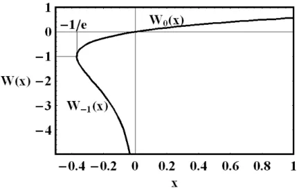
To determine the existence of price solutions, we introduce the Lambert
W-function, Corless et al. (1996). The Lambert function W(x) is the inverse function of x = W eW. For real x, W(x) is defined for x ≥ −1/e and is a
one-to-many function with two branches: the principal branch W0(x), and a
secondary branch W−1(x). The principal branch of the LambertW-function
W0(x) is defined for x ≥ −1/e and takes values in the set [−1,+∞). The
secondary branch of the Lambert W-function W−1(x) is defined for −1/e≤
x < 0 and takes values in the set [−1,−∞), Figure 1.
Proposition 4.1 Consider a stationary age structured population with a constant age independent mortality rate µ > 0. We suppose further that endowments, φ(a) = φ1δ(a−a1), are distributed at a fixed age a = a1 > 0,
andφ1 is a positive constant. We also assume that the rate of time preference
ρ is a non-negative constant and is independent of age and time. Then, Arrow-Debreu equilibrium price solutions exist, and are given by,
p(t) =p1e
−γt
+p2eλ2t (31)
where,
λ2 =
−µ−ρ−γ− a1
1W0(−a1(µ+ρ)e
−a1(µ+ρ)) if a
1(µ+ρ)≥ 1
−µ−ρ−γ− a1
1W−1(−a1(µ+ρ)e
−a1(µ+ρ)
) if a1(µ+ρ)≤ 1
p1 and p2 are constants, and W0 and W−1 are the principal and secondary
branches of the Lambert W-function. Moreover, the constant λ2 can be
pos-itive, negative or zero.
Proof: We first write equation (30) in the form,
δ+x=δea1x
(32)
Figure 1: Graph of the Lambert W-function. The principal branch of the LambertW-function,W0(x), is defined forx≥ −1/eand takes values in the
set [−1,+∞). The secondary branch of the Lambert W-function, W−1(x),
is defined for −1/e≤x <0 and takes values in the set [−1,−∞).
To find other possible solutions of (32), we multiply (32) by (−a1e−a1(δ+x)),
and rearranging the terms, we obtain,
−a1(δ+x)e−a1(δ+x) =−a1δe−a1δ.
With, z = −a1δe−a1δ and W = −a1(δ +x), the above equation is written
as z = W eW, defining the Lambert W-function, and z ≥ −(1/e). As z =
−a1δe−a1δ is independent of x, we can invert the function z =W eW, Figure
1, and we obtain W =W0,−1(z), or, −a1(δ+x) =W0,−1(−a1δe
−a1δ). Then,
the solution of equation (32) in x is,
x=−δ− 1
a1
W0,−1(−a1δe −a1δ
)
or, with x= (λ+γ),
λ2 =
−µ−ρ−γ− a1
1W0(−a1(µ+ρ)e
−a1(µ+ρ)) if a
1(µ+ρ)≥1
−µ−ρ−γ− a1
1W−1(−a1(µ+ρ)e
−a1(µ+ρ)) if a
1(µ+ρ)≤1.
justifies the form of the price solution in the proposition, where p1 and p2
are arbitraty constants. ✷
Proposition 4.1 allows a characterization of the qualitative properties of Arrow-Debreu equilibrium price solutions as functions of behavioural and age-dependent parameters.
The equilibrium price is indeterminate at time t = 0 but can converge asymptotically to zero or to infinity. The indeterminacy of the spot market price is an instance of the Walras law. The case of prices converging to infinity corresponds to the existence of rational speculative bubbles. In this case, the implicit real interest rate (-p1(t)dpdt(t)) is asymptotically negative. If the implicit real interest rate is positive, there are no speculative bubbles.
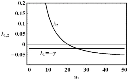
Figure 2: Roots λ1 =−γ and λ2 of equation (30) as a function of a1 — the
age of endowment distribution, for ρ = 0.025, µ = 0.015 and γ = 0.02. By (33), we have,λ2 = 0 for a1 = 20.273.
The equilibrium price solution given in Proposition 4.1, is of the form
p(t) = p1e−γt+p2eλ2t, where λ2 can take any real value. In Figure 2, we
show λ1 = −γ and λ2 as a function of a1, for ρ = 0.025, γ = 0.02 and
µ = 0.015. It suggests that there is a critical ageacri, such that if a1 ≥acri,
then λ2 ≤ 0 and prices will converge asymptotically to zero. If a1 < acri,
then prices will go to infinity and we have a speculative bubble.
solving for a1, we obtain,
acri= 1
γlog 1 + γ µ+ρ
!
(33)
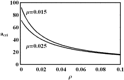
for anyγ ≥0. In the case of stationary endowments (γ = 0), the critical age isacri = 1/R= 1/(µ+ρ)>0. As we can see from Figure 3, the critical age is an inverse function of what we can term the effective psychological discount rate (µ+ρ).
We have shown that the existence of bubbles depends on the magnitudes of the growth rate, of the rate of time preference, of the mortality rate and of the age of distribution of the endowment. That is, bubbles can exist as a result of the interactions between population dynamics and the life-cycle distributions of endowments. These results are a consequence of the balance equation (30): Equation (30) represents the balance between a wealth effect with endowments distributed at age a1 (right-hand side), and the inverse of
the weight of the wealth of all the cohorts at birth (left-hand side). Therefore, if a1 is too large (a1 > acri), the wealth effect is also large, and the balance
between the two terms exists only if λ2 < 0. If a1 < acri, the inverse of
the weight of the wealth of all the cohorts at birth is large, and the balance between the two terms exists only if λ2 >0.
In infinite horizon non-OLG economies, the Arrow-Debreu prices converge to zero, and therefore to a positive interest rate. In OLG models with two-periods lifetime, rational speculative bubbles can arise in the limit t → ∞
(LeRoy (2004)). In the continuous time OLG model developed here, the existence or not of speculative bubbles is determined by an age-dependent distribution of endowments.
4.2
Endowments up to retirement age
We consider now a more realistic case, which is closely related to two-period OLG models. In these models there is no labour income after retirement, and therefore, in that period, consumption must be financed in advance. We consider an endowment distribution such that the dependence of endowments on age is described by the following function,
φ(a) = (
φ1 (0 ≤a < ar)
Figure 3: Critical ageacrias a function of (µ+ρ), forγ = 0.02, and calculated from (33). For example, for (µ+ρ) = 0.01,acri= 54.93, and for (µ+ρ) = 0.02,
acri= 34.66.
where ar is a maximal age of endowments, say, a retirement age, and φ1 is a
constant. In order to search for an Arrow-Debreu price solution in the form (27), we substitute (34) into (28), obtaining the condition for λ,
(µ+ρ+γ+λ)(µ−γ−λ)(1−e−µar
) =µ(µ+ρ)(1−e−µar
e(γ+λ)ar
). (35)
Proposition 4.2 Consider a stationary age structured population with a constant mortality rate µ >0, and suppose that endowments are distributed according to the function (34). Consider also that the rate of time preference isρ >0. Then Arrow-Debreu equilibrium price solutions exist, and are given by,
p(t) =
p1e−γt+p2e(µ−γ)t+p3eλ3t if arµ(µ+ρ)/(1−e−arµ)<2µ+ρ
p1e−γt+p2e(µ−γ)t if arµ(µ+ρ)/(1−e−arµ) = 2µ+ρ
p1e−γt+p2eλ3t+p3e(µ−γ)t if arµ(µ+ρ)/(1−e−arµ)>2µ+ρ
and ρ < µ(µ+ρ)are−arµ/(1−e−arµ)
p1e−γt+p2e(µ−γ)t if ρ=µ(µ+ρ)are−arµ/(1−e−arµ)
p1eλ3t+p2e−γt+p3e(µ−γ)t if ρ > µ(µ+ρ)are−arµ/(1−e−arµ)
where p1, p2 andp3 are arbitrary constants. Equation (35) has at most three
Proof: We first write equation (35) in the form,
(x−µ)(µ+ρ+x) = c(ear(x−µ)
−1) (36)
wherex=λ+γandc=µ(µ+ρ)/(1−e−arµ)>0. We can also write equation
(36) in the form g(x) = f(x). The function g(x) is a quadratic polynomial with roots at x=µ >0 and x=−µ−ρ <0. The function f(x) has a zero at x=µ > 0. The functionsf(x) andg(x) both intersect at the points x= 0 and x=µ. Hence, (35) has at least two solutions,
λ1 =−γ , λ2 =µ−γ
with λ1 < λ2.
The polynomial g(x) has a minimum for x = ¯x =−ρ/2, implying that, ¯
λ = ¯x−γ = −ρ/2−γ < λ1. Therefore, if x > x¯, g(x) and f(x) are both
monotonic increasing functions of x, and equationg(x) =f(x) can have one more solution.
If g′
(0) > f′
(0), equation (35) has a third solution. We denote this solution byλ3, and λ3 < λ2 =−γ. In this case,g′(0)> f′(0) is equivalent to
ρ > care−arµ
. This proves the fifth case in the proposition. If, ρ=care−arµ
, we have only the two roots λ1 and λ2, and the fourth case is proved.
Analogously, if f′
(µ)> g′
(µ), we obtain the first case in the proposition, where λ3 > λ2, and the condition is, car < 2µ+ρ. In the second case we
have only two roots and the condition is car = 2µ +ρ. The third case is
immediate. ✷
The results of Propositions 4.1 and 4.2 are similar, in the sense that the price solutions for the macroeconomic equilibrium are qualitatively the same. In the case analyzed here of a continuous distribution of endowments up to agear, there exists also a critical age,acri, where, forar< acri, the asymptotic price solution goes to infinity, implying the existence of a speculative bubble, Figure 4. In this case, the value ofacrias a function ofρhas been determined numerically, Figure 5.
Figure 4: Roots λ1,2,3 of equation (35) as a function of ar, for ρ =γ = 0.02
and µ= 0.015.
growth rate, on the rate of time preference, and on the mortality rate, Figure 5. If we choose realistic values for the parameters, as for example,γ = 0.02,
ρ = 0.01 and µ = 0.010, the critical age of retirement is acri = 51.08. If we choose γ = 0.02, ρ = 0.01 and µ = 0.005, the age of retirement is
acri = 56.1. Therefore, as the mortality modulus decreases, the critical age avoiding speculative bubbles increases.
5
Conclusions
In this paper, we have derived a continuous time overlapping generations model for an endowment Arrow-Debreu economy with an age-structured po-pulation.
We have proved that in this Arrow-Debreu economy with a balanced growth path, equilibrium prices exist, and there exists a critical age such that, if endowments are distributed earlier than that age, speculative bubbles for prices exist.
Figure 5: Critical age acri as a function of ρ, forγ = 0.02 and several values of the mortality modulus µ. The critical age has been calculated numerically from (36) with x=γ.
Acknowledgments
An earlier version of this paper has been presented at the Viennese Vintage Workshop, hosted by the Vienna Institute of Demography, Austrian Academy of Sciences, 24-25 November 2005. Comments by two anonymous referees have been helpful. We acknowledge the partial support of FCT (Portugal) through pluriannual funding grants to UECE-ISEG and to GDNL-IST.
References
Azariadis, C., Bullard, J., and Ohanian, L. (2004). Trend-reverting fluctua-tions in the life-cycle model. Journal of Economic Theory, 119: 334–356.
Balasko, Y. and Shell, K. (1980). The overlapping-generations model, I: The case of pure exchange without money. Journal of Economic Theory, 23: 281–306.
Blanchard, O. J. (1985). Debt, Deficits and Finite Horizons. Journal of Political Economy, 93(2): 223–47.
Bommier, A. and Lee, R. D. (2003). Overlapping Generations Models with Realistic Demography: Statics and Dynamics. Journal of Population Eco-nomics, 16: 135–60.
Boucekkine, R., de la Croix, D., and Licandro, O. (2002). Vintage human capital, demographic trends and endogenous growth. Journal of Economic Theory, 104: 340–75.
Cass, D. and Yaari, M. E. (1967). Individual saving, aggregate capital accu-mulation, and efficient growth. In Shell, K., editor, Essays on the Theory of Optimal Economic Growth, pages 233–268. MIT Press.
Corless, R. M., Gonnet, G., Hare, D. E. G., Jeffrey, D. J., and Knuth, D. E. (1996). On the Lambert W Function. Advances in Computational Mathe-matics, 5: 329–59.
Cushing, J. M. (1998). An introduction to structured population dynamics. SIAM, Philadelphia.
d’Albis, H. and Augeraud-Veron, E. (2004). Competitive growth in a life-cycle model: existence and dynamics. ftp://mse.univ-paris1.fr/pub/mse/cahiers2004/V04016.pdf.
Demichelis, S. and Polemarchakis, H. M. (2006). The determinacy of equi-librium in economies of overlapping generations. Economic Theory, forth-coming.
Diamond, P. A. (1965). National Debt in a Neoclassical Growth Model. American Economic Review, 55(5): 1126–1150.
Dil˜ao, R. (2006). Mathematical models in population dynamics and ecology. In Misra, J. C., editor,Biomathematics: Modelling and Simulation. World Scientific.
Gale, D. (1973). Pure exchange equilibrium of dynamic economic models. J. Econ. Theory, 6: 12–36.
Galor, O. and Weil, D. (2000). Population, Technology, and Growth: From the Malthusian Regime to the Demographic Transition and Beyond. Amer-ican Economic Review, 90(4): 806–828.
Geanakoplos, J., Magill, M., and Quinzii, M. (2004). Demography and the long-run predictability of the stock market.Brookings Papers on Economic Activity, 1, 241-307.
Geanakoplos, J. D. and Polemarchakis, H. M. (1991). Overlapping gener-ations. In Hildenbrand, W. and Sonnenschein, H., editors, Handbook of Mathematical Economics, volume IV, pages 1899–1960. North Holland.
Lanczos, C. (1970). The variational principles of mechanics. University of Toronto Press, Toronto.
LeRoy, S. F. (2004). Rational exuberance . Journal of Economic Literature, 42: 783-804.
Lindh, T. and Malmberg, B. (1999). Age Structure Effects and Growth in the OECD, 1950-90. Journal of Population Economics, 12: 431–99.
McKendrick, A. G. (1926). Applications of mathematics to medical problems. Proceedings of the Edinburgh Mathematical Society, 44: 98–130.
Poterba, J. M. (2001). Demographic structure and asset returns. Review of Economic and Statistics, 83: 565–584.
Radner, R. Existence of equilibrium of plans, prices, and price expectations in a sequence of markets Econometrica, 40: 289–303.
Samuelson, P. A. (1958). An Exact Consumption-Loan Model of Interest with or Without the Social Contrivance of Money. Journal of Political Economy, 66(6): 467–82.
Shell, K. (1971). Notes on the economics of infinity. Journal of Political Economy, 79: 1002–1011.