ADVANCE
–
Centro de Investigação Avançada do ISEG
“
CDOs in the Light of the Current Crisis
”
WORKING PAPER N. 2 /2008
June 2008
Abstract
This paper proposes a top-down model for pricing Collateralized Debt Obligation (CDOs). Our proposal is both treatable and realistic, in the sense we are able to obtain closed-form solutions to single tranche CDOs and capturing extreme credit events. We use as key ingredients the so-called (T, x)-bonds, as proposed in Filipovic, Overbeck, and Schmidt (2008), but generalize their affine specificationby including shot-noise processes.
Our claim is that affine diffusions combined with shot-noise processes lead to an improved modeling of CDO spreads in comparison to existing affine jump-diffusion models. The proposed approach allows in particular for better capturing the possibility of extreme events, like the ones underlying the current crisis. We illustrate our results with a very concrete (simple) instance of our class of models. Finally, we identify the connections between the top-down and bottom-up approaches for modeling credit risk, within our class of models. Concretely, we show that even when taking a bottom-up approach the aggregate loss process would be a process of affine shot-noise type.
Key words: CDO; Shot-noise processes; affine models.
JEL Classification: C15,C12, G13, G33
.
Raquel M. Gaspar
ADVANCE Research Center
ISEG, Technical University of Lisbon
R. Miguel Lupi, 20,1249-078 Lisbon,
Portugal
Email: Rmgaspar@iseg.utl.pt
Thorsten Schmidt
Department of Mathematics,
University of Leipzig
D-04081 Leipzig,
Germany
Raquel M. Gaspar1 and Thorsten Schmidt2
June 2008
Abstract
This paper proposes a top-down model for pricing Collateralized Debt Obligation (CDOs). Our proposal is both treatable and realistic, in the sense we are able to obtain closed-form solutions to single tranche CDOs and capturing extreme credit events. We use as key ingredients the so-called (T, x)-bonds, as proposed in Fil-ipovi´c, Overbeck, and Schmidt (2008), but generalize their affine specification by including shot-noise processes.
Our claim is that affine diffusions combined with shot-noise processes lead to an improved modeling of CDO spreads in comparison to existing affine jump-diffusion models. The proposed approach allows in particular for better capturing the pos-sibility of extreme events, like the ones underlying the current crisis. We illustrate our results with a very concrete (simple) instance of our class of models. Finally, we identify the connections between the top-down and bottom-up approaches for modeling credit risk, within our class of models. In particular, we show that even when taking a bottom-up approach the aggregate loss process would be a process of affine shot-noise type.
1. Introduction
A collateralized debt obligation (CDO) is a security backed by a pool of reference entities such as bonds, loans or credit default swaps (CDSs). The reference entities form theasset sideof the CDO. Issued notes on tranches of different seniority build the liability side of the CDO. A CDO is, therefore, a derivative on a portfolio of
N credit risky instruments. CDO markets have experience great growth during the last decade. Nowadays the most liquidly traded CDOs are based upon so-called credit indices that were created in 2004 – the CDX for North-America and the Itraxx for Europe. Fore more details and references on credit risk products and markets we refer to the respective chapters in McNeil, Frey, and Embrechts (2005). The valuation of CDOs tranches is far from trivial and relies considerably on the default correlation between the various reference entities in the pool. Copula models have emerged as a way to deal with such correlations. The one-factor Gaussian copula approach is, still nowadays, the industry standard. See e.g. Laurent and Gregory (2005). Copula models, however, have serious limitations (mainly due to their non–dynamic nature) and have been quite heavily criticized both in the academic world and, more recently in connection to the credit risk crisis, also in the industry. For more details on copula models we refer to the appropriate chapter in Sch¨onbucher (2003).
Reduced-form models of credit risk have been popular for pricing of single-name credit products. The question of how to extend them multi-name case is of great interest. Two alternative approaches have emerged : the bottom-up approach and the top-down approach.
In the bottom-up approach the credit risk of each reference entity is modeled as well as all default correlations. To arrive to the loss process associated with the
1Advance Research Center, ISEG, Technical University of Lisbon, PORTUGAL.
E-mail:Rmgaspar@iseg.utl.pt
2Department of Mathematics, University of Leipzig, D-04081 Leipzig, GERMANY. Email:
tschmidt@math.uni-leipzig.de
CDO we need to aggregate all this information. This approach has great flexibility, as it allows to consider the specificities of each entity separately as well as their connections, but lead to non parsimonious models that can be hard to calibrate to market data. The top-down approach models the credit risk of the entire pool at once. See Giesecke and Goldeberg (2007). If we are interested only in the behavior of the entire pool this is sufficient and lead to dynamic and parsimonious models. The need of parsimonious alternatives to the copula models and the development of credit risk markets made the top-down approach more and more popular. Specially with the appearance of standardized credit indices and liquidly traded derivative products written on those indices. Despite their philosophical differences, it is quite straightforward to apply mathematical methods used in one approach to develop a model belonging to the other approach.
Here we take a top-down approach and extend the well-known class of affine models (see e.g.Duffie, Filipovi´c, and Schachermayer (2003), Singleton and Umant-sev (2002) or Filipovi´c, Overbeck, and Schmidt (2008)) by a shot-noise process as proposed by Gaspar and Schmidt (2007). The show that the shot-noise effect is par-ticularly important to guarantee extreme movements like the ones recently observed in credit markets.
The remaining of the paper is organized as follows. In Section 2 we present the mathematical formalism proposed by Filipovi´c, Overbeck, and Schmidt (2008), useful when dealing with CDOs. In Section 3 we present the affine shot-noise setup and show how to obtain the distribution of the loss process, prices of (T, x)–bonds and, thus, CDO tranche spreads in closed-form. We study the link between the top-down and bottom-up approach in our setup and show that affine shot-noise intensities of individual names lead to affine shot-noise loss processes. Finally we discuss measure changes and calibration issues. In Section 4 we compare a concrete instance of our class of models with the model proposed by Duffie and Gˆarleanu (2001) and argue ours is more flexible and can capture better extreme events like the ones recently experienced in credit risk markets.
2. Collateralized Debt Obligations
Consider a complete filtered probability space (Ω,F,(Ft)t≥0,P) satisfying the
usual conditions. We directly work under an equivalent martingale measure Q. The measure change from the real-world measurePto Qis quite standard and we give more details in Section 3.5.
The total nominal of the CDO is normalized to one. Let L = (Lt)t≥0 be the
process of accumulated losses over time. This is a pure-jump process which jumps default of entities in the pool by the size of the occurred loss. A special case, quite often considered in practice, is where the loss on each default is a constant. By
I = [0,1] we denote the set of attainable loss fractions3.
As in Filipovi´c, Overbeck, and Schmidt (2008) we consider defaultable (T, x)– bonds, which pay one if the aggregated CDO loss process has not exceeded x at maturity T and zero else, as basic constituents. A (T, x)–bond has a payoff of
1{Lt≤x} at maturity T, for x ∈ I. We denote its price, at time t by p(t, T, x)
Note that p(t, T, x) is decreasing in T and increasing in x. For x= 1 we obtain
p(t, T,1) =:p(t, T), i.e. the price of a default-free bond.
Knowledge of prices of all (T, x)-bonds is sufficient for pricing derivatives on the loss process. Indeed, consider the payoff
F(LT) =F(1)−
1 Z
0
F′(y)1{LT≤y}dy
for some bounded measurable functionF′. A Fubini argument shows that the price
of a derivative offeringF(LT) atT is given by
F(1)p(t, T)− 1 Z
0
F′(y)p(t, T, y)dy.
Investing in CDOs is done via a so-called single-tranche CDO (STCDO), sometimes also called tranche credit default swap. A STCDO is represented by its lower and upper detachment points, x1 and x2, with 0≤x1< x2≤1. The investor receives
coupon payments at times T1, . . . , Tn. In exchange, the investor covers a certain
part of the occurring losses. Set
G(x) := (x2−x)+−(x1−x)+= Z
(x1,x2]
1{x≤y}dy.
Then, investing in the STCDO with swap rate S is equivalent to the following payment stream:
(1) Payment leg. The investor receives atS G(LTi) atTi, i= 1, . . . , n.
(2) Default leg. The investor pays−dG(Lt) =G(Lt−)−G(Lt) at default times
(any time where ∆Lt6= 0).
In Filipovi´c, Overbeck, and Schmidt (2008) it is shown that the value of the STCDO at time tcan be derived solely on the basis of (T, x)-bonds, and is given by
V(t, S) =
Z
(x1,x2]
1{Lt≤y} S n X
i=1
p(t, Ti, y) +p(t, Tn, y)−p(t, T0, y) +γ(t, y) !
dy,
where γ(t, y) =
Tn Z
T0
EQhrue− Ru
t rsds1
{Lu≤y}|Ft i
du. (1)
In the case where default-free interest rates and the loss process are independent,
γ(t, T) simplifies toγ(t, y) =RTn
T0 f(t, u)p(t, u, y)du where f(t, u) denotes the
risk-free forward rate. Setting V = 0 and solving for S gives the par-spread for this investment. Under this assumption we also have
p(t, T, x) =p(t, T)EQ1{LT≤x}|Ft
. (2)
3. The Affine Shot-Noise Setting
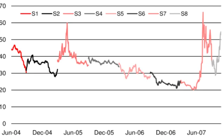
The current crisis shows a dramatic behavior of spreads of credit indices like iTraxx or CDX. In Figure 1 we show data from the iTraxx. The purpose of this paper is to propose a simple model which is able to capture the dramatic increase in spreads.
Typically, in credit indices like iTraxx, the underlying entities have zero recovery for each defaultable instrument. We assume that there are N constituents of the credit pool an so the loss process Ljumps byδ=N−1 at each default. We assume
that L is a conditional Markov process, which in our framework implies that N
is δ times a Cox process with a given intensity, say λunder Q. with λ(t, x)). As outlined above it is sufficient to price (T, x)–bonds for pricing STCDOs. We assume the risk-free rate of interest is independent of λ. This is a typical assumption in credit risk4. Also note that, since at each default time the nominal amount reduces
4All formulas can be derived without these assumptions, most expectations would then need to
0 10 20 30 40 50 60 70
Jun-04 Dec-04 Jun-05 Dec-05 Jun-06 Dec-06 Jun-07
S1 S2 S3 S4 S5 S6 S7 S8
Figure 1. A graph of rolled-over iTraxx spreads. A diffusive movement as well as high price peaks are a typical characteristics of the spreads.
byδ, we can easily keep track of the numbers of defaults occurred, up to any time
t as they are given by the ratioLt/δ and the expectation in (2), simplify to
QLT ≤x|Ft
=1{Lt≤x}
(x−Lt)/δ X
n=0
Q(LT−Lt=nδ|Ft) (3)
wherengives us the number of jumps (defaults) in the interval (t, T]. So, it suffices to compute the risk-neutral probability for all possible ndefaults occurring in the interval (t, T], i.e. n= 0,· · · ,(x−Lt)/δ.
3.1. Setup. The class of models here proposed results from a combination of con-tinuous affine processes with shot-noise processes. Concretely, we assume that
λt=ηt+Jt (4)
where η andJ are some continuous and pure jump processes, respectively.
(A1): AssumeJ is an exponentially declining shot-noise process, i.e.
Jt= X
˜
τi≤t
Yih(t−˜τi). (5)
Here Yi, i = 1,2, . . . are i.i.d., independent of everything else and ˜τi are
the jump times of a Poisson process with intensity l and we takeh(x) = exp(−cx). Phrased in different words, J is a mean-reverting compound Poisson process.
(A2): Assumeη is a continuous affine process, i.e
ηt=g(t)⊤Zt+f(t) (6)
forZ ≥0 the m-dimensional vector of state variables that uniquely solves
dZt=α(t, Zt)dt+σ(t, Zt)dWt.
Here W is a n-dimensional Q–Wiener process. α : R+×Rm 7→ Rm and
σ:R+×Rm7→Rn×n are such that
α(t, z) =d(t) +E(t)z (7)
σ(t, z)σ⊤(t, z) =k0(t) +
m X
i=1
ki(t)zi (8)
f, g, dand E, k0, ki (fori= 1,· · · , m) are smooth functions mapping R+
A typical example, at which we look more closely in Section 4, satisfying (A2) is the one-factor CIR-process where η=Z and it hasQ-dynamics given by
dηt=κ(b−ηt)dt+σ√ηtdWt.
More general dynamics, for example to include various factors, can be easily incor-porated in the setting given by (A2).
Comparing to Figure 1, assumptions (A1) and (A2) seem very reasonable. A diffusive part which captures the risk of smaller movements in λ. The shot-noise part captures the heavy reactions of the market to news like in the current crisis. General choices ofhallow to capture different modeling aspects but, for simplicity, we concentrate on exponentially declining h.5
3.2. Loss Process distribution. The following proposition gives a closed-form expression for the conditional (an unconditional) risk-neutral distribution function of loss process L. The proof is provided in the appendix. From this result we immediately obtain prices of (T, x)-bonds and hence of STCDOs (equations (2) and (1), respectively).
Proposition 3.1. Consider the affine shot-noise setting. Then
QLT ≤x|Ft
=1{Lt≤x} x−Lt
X
k=0
1
k!
∂kS(θ, t, T)
∂θn
θ=−1
(9)
where S(θ, t, T) = exp
A(θ, t, T) +B⊤(θ, t, T)Zt+C(θ, t, T)Jt+D(θ, t, T) .
A and B on R×R+×R+ are deterministic in R and Rm, respectively, solving
system of Riccati equations, for allθ∈R andt≤T
∂A ∂t +d
⊤(t)B+1
2B
⊤k
0(t)B=−θf(t) (10)
∂B ∂t +E
⊤(t)B+1
2B˜
⊤K(t)B=
−θg(t) (11)
subject to the boundary conditions A(θ, T, T) = 0, B(θ, T, T) = 0. A and B should always be evaluated at(θ, t, T). f, gare as in (6) andE,d,k0, are as in (7)-(8),while
˜
B andK(t)∈Rm2×m are simply
˜
B:=
B 0 · · · 0
0 B · · · 0
..
. . ..
0 · · · 0 B
, K(t) =
k1(t)
.. .
km(t)
.
C and D onR×R+×R+ are also deterministic in Rand given by
C(θ, t, T) = θ
c
1−e−c(T−t) (12)
D(θ, t, T) = l· ZT
t
ϕθ c 1−e
−c(T−u)
du−(T−t)
(13)
with ϕ(u) :=E(exp(uY1))the Laplace transform of Y1.
5It is possible to be quite general for the choice ofh. However, ifhis not of the exponential
3.3. Calibration issues. It is far beyond the scope of this paper to provide a calibration of the model to observed prices of credit indices as this is indeed a com-putationally difficult task. However, recently there emerged some calibration results of top-down approaches in the literature. One of the most important contributions in this direction is the work of Cont and Minca (2008). They introduce the so-called effective intensity λeff(t, Lt) = E(λt|Lt) and calibrate it in a non parametric way
to observed index prices. They show that qualitatively, the market implied λeff is
increasing for smallL, stays on a plateaux for intermediate Land finally decrease. We show how to computeλeff in our case and give an intuition how this behavior
can be replicated in our setup. In the next proposition we compute λeff in our
setting and show that this form can indeed be achieved. A proof is given in the appendix.
Proposition 3.2. In the affine shot-noise setting
λeff(t, k) =E(λt|Lt=k) = ∂k ∂θk
θ=−1
∂ ∂t
1
θS(θ,0, t)
k! ∂k ∂θk
θ=−1S(θ,0, t)
Qualitatively, it is quite intuitive, that λeff will first increase sharply and then
stay on a medium level in our setup. This is because λt is not observed andLtis
used as a statistic to estimate it (in the conditional expectation,λeff). IfLtincreases
this comes as a surprise ifλtwere small. The conditional distribution therefore will
be updated strongly which explains a first sharp rise. IfLincreases further, this is no longer such a big surprise and this effect vanishes.
3.4. Relation to the bottom-up approach. In this section we show that a bottom-up approach based on conditionally independent defaults with a factor structure, where the factors consists of affine and shot-noise processes lead to a jump intensityλof the loss process as proposed in Assumptions (A1)-(A2).
We say a process µ= (η, J) satisfying (A1) and (A2) is shot-noise linear with parameters (g, f, c, l, F) where F denotes the distribution ofY1. A special case of
Proposition 4.3 in Gaspar and Schmidt (2007) tells that the sum of two shot-noise linear processes is itself shot-noise linear. Thus, by induction, the sum of a finite number of such processes will also be shot-noise linear.
Proposition 3.3. Consider two independent processes µ1 andµ2, both shot-noise
linear with parameters (g1, f1, c, l1, F1)and(g2, f2, c, l2, F2), respectively. Setq:=
l1(l1+l2)−1. Thenµ1+µ2is shot-noise linear with parameters(g1+g2, f1+f2, l1+
l2, c, qF1+ (1−q)F2).
For bottom-up modeling with the affine shot-noise setting, we propose the fol-lowing approach. Consider m companies. Assume that their default times are conditionally independent with default intensitiesλ1, . . . , λm.
For each companyi, take
λit=
gi(t) +ǫi1g(t) ⊤
Zt+fi(t) +ǫi2J(t). (14)
Note that in the above expression we suppose the specific default risk of each firm is only affected by the affine diffusion processes Z (through the functions gi and
fi) while the common (systematic) risk is affected by both affine processes and a
shot-noise processes (throughf,gandJ). The parametersǫi
1, ǫi2allow us to control
for different sensitivities of the companies to the common factors.
By settingǫj :=Pmi=1ǫij, it is easy to show that in this case the jump intensity
of the loss process isλt=Pmi=1λit. Due to Proposition 3.3λis the shot-noise linear
and given the specification in (14) its parameters are (Pm
i=1gi+ǫ1g,
Pm
i=1fi, c, l, F∗)
where F∗ is the distribution ofǫ
2Y.6
3.5. Measure Changes. Up to now we always assumed thatQwas a risk-neutral measure. It is of course possible to consider the proposed model with respective to some objective probability measure P∼Q. In particular this is necessary for the computation of risk measures and statistical analysis of the model. In the considered framework it is reasonable to assume that the model is also shot-noise linear under
P, which restricts the class of equivalent probability measures. A measure change from Qto Pwill then have the following impact:
d(·), E(·)❀d˜(·), E˜(·)
l, FY ❀˜l,F˜Y
for some appropriate deterministic functions ˜d,E˜, constant ˜l >0 and distribution function ofY underP, ˜FY. Note that this kind of measure change leavesY1, Y2, . . .
i.i.d. underP. For a general reference see Theorem III.3.24 in Jacod and Shiryaev (1987).
4. A Concrete (simple) Example
In this section we use a concrete instance of our class of models to illustrate the results previously derived. We present only the main results but more details about the computations can be found in the appendix. We then compare our concrete instance with a model proposed by Duffie and Gˆarleanu (2001).
Recall that λt=ηt+Jt. Consider the following instance of our class of models:
(i) Z =η with the following dynamics
dηt=κ(b−ηt)dt+σ√ηtdWt
(ii) Jt= X
˜
τi≤t
Yiexp(−c(t−τ˜i)) whereY1, Y2, . . . are i.i.d.χ2(2)-distributed.
Under (i)-(ii), A(θ, t, T),B(θ, t, T) andD(θ, t, T) withθ < 2κσ22 are given by7
A(θ, t, T) = 2κb
σ2 ln
(ψ−κ)
eψ(T−t)−1
+ 2ψ
2ψe(ψ−κ)(T−t) 2
!
B(θ, t, T) = 2θ
eψ(T−t)−1
(ψ−κ)
eψ(T−t)−1
+ 2ψ
D(θ, t, T) = l
c(T−t)−ln
1 + 2θ c e
−c(T−t)−1
c−2θ −(T−t)
where ψ=√κ2−2σ2θ.
We take this simple example to illustrate the applicability of our approach. The full implementation and comparison to data is far beyond the scope of this paper. However, the expressions obtained up to now relate on sums of certain derivatives and the question may be raised, how to compute these in practise. As our main goal is to emphasize the importance of shot-noise processes, we concentrate on the terms regarding the shot-noise part.
6Note that we did not needed to use the result of Proposition 3.3 for the sum of the shot-noise
-5 -4 -3 -2 -1 1
Θ
0.9 1.0 1.1 1.2 1.3
SJ
c=10 c=8 c=4
Figure 2. The plot shows SD(θ, t, T) = exp(D(θ, t, T)) which is,
forθ=−1, the probability of no loss in (t, T]. l has the value 0.4.
-1.8 -1.6 -1.4 -1.2 -1.0 -0.8 -0.6
Θ
0.06 0.08 0.10 0.12 0.14 DΘHSJL
c=10 c=8 c=4
-1.8 -1.6 -1.4 -1.2 -1.0 -0.8 -0.6
Θ
0.04 0.06 0.08 0.10 DΘ
2H
SJL
c=10 c=8 c=4
Figure 3. The plot shows the first and second derivative ofSD(θ, t, T)
Without loss of generality we assume thatJt= 0, i.e. there were no past jumps.
Then to obtain the shot-noise impact on the loss distribution given in (9), we have to compute
x−Lt X
k=0
1
k!
∂kexp(D(θ, t, T))
∂θn
θ=−1
where SD(θ, t, T) := exp(D(θ, t, T)). For θ=−1,SD denotes the probability that
in (t, T] no jump happens. In the single-name case this would be the survival probability. As by intuition,SD has the following properties: first, it is increasing
in c: if c = 0, jumps persist forever and J is strictly increasing. If c is large, the effect of a jump vanishes very fast and J is pulled back to zero, so for largec we will see less defaults and so the probability of having no default in (t, T] clearly increases. Second, it is decreasing inl: if the intensity of jumps inJ increases, this immediately decreases the probability of no default in (t, T]. Forl= 0.4 we plot the function and its first two derivatives in Figure 2 and Figure 3, respectively. Note that the derivatives are quite small, in particular atθ=−1. This together with the factor (k!)−1implies that the crucial impact is reasonably measured by considering
a few terms of the above sum.
Of course, the DG model considered from a bottom-up approach leads to a model forλwhich has an inherent factor structure. This approach has in principle the same tractability as the approach outlined here, but formulas get much more involved. How to achieve this is described in full detail in Gaspar and Schmidt (2007).
Appendix A. proofs
Proof of Proposition 3.1. The proof heavily relies on the independence of η and J
and uses the techniques set out in Gaspar and Schmidt (2007). Given (3) it suffices to show that
Q(LT −Lt=k|Ft) = 1
k!
∂kS(θ, t, T)
∂θk θ=−1
(15)
LetRT
t λsds=: Λ(t, T). Using conditional independent increments we have
Q(LT−Lt=k|Ft) =EQ
exp(−Λ(t, T))(Λ(t, T))
k
k! |Ft
.
In the following we useE(AneθA) = ∂k
∂θkE(e
θA),forθ∈R, such that the expectation
and their derivatives exist. Thus,
EQexp(−Λ(t, T))(Λ(t, T))k Ft = ∂ k ∂θk θ=−1E
Q
exp(θΛ(t, T) Ft
(16)
Moreover, Λ(t, T) =RT
t (ηs+Js)ds, withη andJ being independent. Hence,
(16) = ∂
k
∂θk
θ=−1
Sη(θ, t, T)SJ(θ, t, T)
withSη(θ, t, T) :=EQ
e−θRT t ηsds
Ft
andSJ(θ, t, T) :=EQ
e−θRT t Jsds
Ft
. First, using standard results from affine term structures (see, e.g. Bingham and Kiesel (1998)) and the fact that η is an affine function of and affine process Z, we get
Sη(θ, t, T) = expA(θ, t, T) +B⊤(θ, t, T)Zt
where A, B solve (10)-(11). Second,
T Z
t
Judu= X
τi≤t
Yi T Z
t
e−c(u−τi)du+ X τi∈(t,T]
Yi T Z
τi
e−c(u−τi)du
=X
τi≤t
Yi
e−c(t−τi)−e−c(T−τi)
c +
X
τi∈(t,T]
Yi
1−e−c(T−τi)
c .
Note that the first term is measurable w.r.t.Ftand equalsC(1, t, T)JtwithCas in
(12). To compute the expectation containing the second part, we condition on the number of jumps in the interval (t, T] and use the well-known fact that then jump times have the same distribution as order statistics from i.i.d. uniform (t, T]-random variables. Hence, η1, η2, . . . being uniform (t, T],
E
exp X
τi∈(t,T)
θYi
c 1−e
−c(T−τi)
=e−l(T−t)X
k≥0
(l(T−t))k
k! E
exp k X i=1 θYi
c 1−e
−c(T−τi)
Observe that withη1uniform on (t, T], EQ exp θY 1
c 1−e
−c(T−τi)
= 1
T −t
T Z
t
ϕθ c 1−e
−c(T−u)
du
and we find
SJ(θ, t, T) =EQ
eRtTθJsds |FtJ
= exp
C(θ, t, T)Jt+l(T−t) h
−1 + 1
T−t
T Z
t
ϕθ c 1−e
−c(T−u)i
= expC(θ, t, T)Jt+D(θ, t, T)
.
Proof of Proposition 3.2. We have to compute the conditional distribution of λt
given only the number of jumps. Using Bayes’ rule we have that
E(λt|Lt=k) =
E(λt1{Lt=k}) Q(Lt=k)
.
Recall that under the conditional independence assumptionLtis Poisson (Λ(0, t)).
Then, using (15),
Q(Lt=k) =
∂k
∂θk
θ=−1S(θ,0, t).
Let us denote Λ(0, t) =Rt
0λsds= Λ(t). To computeE(λt1{Lt=k}) note that
E(λt1{Lt=k}) =E
λtexp(−Λ(t))
Λ(t)k
k! = 1 k! ∂k ∂θk
θ=−1 1
θ ∂ ∂tE
exp θΛ(t) = 1 k! ∂k ∂θk
θ=−1
∂ ∂t
1
θS(θ,0, t).
Appendix B. Example - some computations
In our concrete illustration, the system of ODEs in (10)-(11) reduces to
∂A
∂t(θ, t, T) +κbB(θ, t, T) = 0 ∂B
∂t(θ, t, T) +κB+
1 2σ
2B2(θ, t, T) = −θ
with the boundary conditions A(θ, T, T) = 0, A(θ, T, T) = 0 for all θ. The second ODE is a scalar Ricatti equation with well-known solution.
B(θ, t, T) = 2θ
eψ(T−t)−1
(ψ−κ)
eψ(T−t)−1
+ 2ψ
withψ=√κ2−2σ2θ. GivenB,Acan then be obtained by simple integration.8
A(θ, t, T) =κb
T Z
t
B(θ, u, T)du=2κb
σ2 ln
(ψ−κ)
eψ(T−t)−1
+ 2ψ
2ψe(ψ−κ)(T−t) 2
!
8A detailed treatment of solutions for scalar Riccatti equations and how to compute some
To compute D we make use of the Laplace transform of the χ2(2) distribution 9.
Foru <0.5 this isϕ(u) =E(euχ2ν) = (1−2u)−1.Then we need to compute
D(θ, t, T) =l
T Z
t
ϕ
θ c
1−e−c(T−u)
du−(T−t)
.
The integral equals
T Z
t
1
1−2θc(1−e−c(T−u)) du=
T Z
t
1
K1+K2exp(cu)
du, (17)
where K1= 1−2θc andK2= 2θcexp(−cT). Thus,
(17) = ln K2+K1e
−ct−ln K
2+K1e−cT
K1c
= c(T−t)−ln
1 + 2θc e−c(T−t)−1
c−2θ
and we obtain that
D(θ, t, T) =l
c(T−t)−ln
1 + 2θc e−c(T−t)−1
c−2θ −(T−t)
.
References
Bingham, N. H. and R. Kiesel (1998). Risk-Neutral Valuation. Springer Verlag. Berlin Heidelberg New York.
Cont, R. and A. Minca (2008). Recovering portfolio default intensities implied by CDO quotes. Columbia University Center for Financial Engineering, Financial Engineering Report No. 2008-01. Also available at SSRN.
Duffie, D., D. Filipovi´c, and W. Schachermayer (2003). Affine processes and ap-plications to finance.The Annals of Applied Probability 13, 984–1053. Duffie, D. and Gˆarleanu (2001). Risk and valuation of collateralized debt
obliga-tions.Financial Analysts Journal 57(1), 41–59.
Filipovi´c, D., L. Overbeck, and T. Schmidt (2008). The term structure of CDO losses. Working Paper.
Gaspar, R. M. (2006). Credit Risk and Forward Price Models. Ph. D. thesis, Stockholm School of Economics.
Gaspar, R. M. and T. Schmidt (2007). Term structure models with shot-noise effects. Advance Working Paper Series n.3/2007, ISEG Technical University of Lisbon. Also available at SSRN.
Giesecke, K. and L. Goldeberg (2007). A top down approach to multi-name credit. Working Paper available at SSRN.
Jacod, J. and A. N. Shiryaev (1987). Limit Theorems for Stochastic Processes. Springer-Verlag.
Laurent, J. and J. Gregory (2005). Basket default swaps, CDOs and factor cop-ulas.Journal of Risk 7, 103–122.
McNeil, A., R. Frey, and P. Embrechts (2005).Quantitative Risk Management: Concepts, Techniques and Tools. Princeton University Press.
Sch¨onbucher, P. (2003). Credit derivatives pricing models - models, pricing and implementation. John Wiley & Sons. New York.
Singleton, K. and L. Umantsev (2002). Pricing coupon-bond options and swap-tions in affine term structure models.Mathematical Finance 12, 427–446.
9Recall that for u ≥0 the Laplace transform of random variable which hasχ2 distribution