ADVANCE

(1)

–

Centro de Investigação Avançada do ISEG

“

Value Investing: The Book-To-Market Effect, Accounting Information,

and Stock Returns

”

Working Paper N. 1 / 2008

January, 2008

Abstract

Although the book-to-market (B/M) effect is vastly studied, the majority of the conclusions in prior analysis is only applicable to U.S. firms. In this work, we evaluate the performance of portfolios selected using three modified versions of B/M strategy applied to stocks listed in Euronext markets (Paris, Amsterdam, Brussels, and Lisbon) between 1993 and 2003. From the analysis of 4,715 firms across 11 years, 943 firms were elected as reference for portfolio formation.

The modified B/M strategies use accounting information to segregate good from troubled firms. The first strategy follows Piotroski's (2000) nine signals to measure three areas of the

companies’ financial situation and enabling to select firms from the high B/M quintile. The

second strategy creates a portfolio from the intersection of high B/M portfolio with low accruals portfolios, following Bartov and Kim (2004) research design. The last strategy combines high B/M and low probability of bankruptcy, using the methodology described in Altman (1968) and Hillegeist et al. (2004).

David Almas

Technical University of Lisbon School of Economics and Management

Rua Miguel Lupi, 20 1249-078, Lisbon, Portugal

davidalmas@gmail.com

João Duque

Technical University of Lisbon School of Economics and Management

Rua Miguel Lupi, 20 1249-078, Lisbon, Portugal

jduque@iseg.utl.pt

(2)

This study shows that the average annual return observed by the high B/M portfolio is increased by 9.2% using the strategy developed by Piotroski (2000). Furthermore, there is clear evidence that the entire high B/M firms return distribution is shifted to the right when the score screen is applied. By opposition, other suggested alternative techniques pointed out in the literature using similar accounting and market data failed to prove as being a more efficient investment strategy

Key words: book-to-market, market efficiency, mispricing, financial statement analysis.

(3)

1. INTRODUCTION

Value investing concerns buying (selling) stocks when their price is low (high) in relation to benchmarks such as earnings, cash flow, dividends, accounting book value, and

historical prices. This approach assumes that while the “true” value for stocks is

measurable and stable, their market prices fluctuate excessively in result of overoptimism or overpessimism, and short-term speculation, among other factors. Value investing is referenced as the opposite of glamour investing, where stocks are bought (sold) when their price is high (low) relative to fundamental benchmarks.

Since Graham and Dodd (1934) that value investing is pointed as able to produce superior stock returns than glamour strategies and the overall market. The purpose of this study is to test specific value investing strategies, using the book-to-market (B/M) effect. The B/M ratio is calculated by dividing the accounting book value of equity by the market value of equity. According to prior research, a portfolio of high B/M firms outperforms a portfolio of low B/M firms and the overall market. Three modified B/M strategies that attempt to exclude a subset of firms for which the B/M signal is likely to be noise are examined in this work. Prior studies that compare different value strategies concluded that high B/M strategies produce better results over the long-term (Chan, Hamao, and Lakonishok (1991)).

The goal of this paper is to test if an investor can achieve a higher return over the long-run by using a simple accounting-based fundamental analysis strategy. If this can be obtained, then there will be evidence of some market inefficiency, since the information under use is widely available.

(4)

performances are then compared against all stocks listed on Euronext, using market-adjusted returns.

This paper is organised as follows: we start by presenting the relevant literature, then we discuss the methodology and the data used, and finally we present the empirical results. We conclude by summarising the results and pointing out some plausible future research paths.

2. LITERATURE REVIEW

Investment analysts have argued that value strategies outperform the market (Graham and Dodd (1934) and Dreman (1977)) for a long time. These claims have intrigued scholars since they are inconsistent with the market efficiency weak form hypothesis. In an effort to evaluate the validity of these claims, academics investigated the performance of value strategies, finding a number of strategies that produce superior returns over the long-run. Basu (1977), Jaffe, Keim, and Westerfield (1989), Chan, Hamao, and Lakonishok (1991), and Fama and French (1992) show that stocks with high earnings-to-price ratios achieve higher returns. De Bondt and Thaler (1985, 1987) argue that extreme losers during a period of time outperform the market over the subsequent time period. Despite some criticism (Chan (1988) and Ball and Kothari (1989)), their conclusions had resisted testing (Chopra, Lakonishok, and Ritter (1992)). Stattman (1980) and Rosenberg, Reid, and Lanstein (1984) find that average returns on U.S. shares are positively connected to the ratio between a firm's book value and the market value for common equity, according to Fama and French (1992) who extended previous results. Chan, Hamao, and Lakonishok (1991) and Lakonishok, Shleifer, and Vishny (1994) have also refined those conclusions. Finally, Chan, Hamao, and Lakonishok (1991) show that a high ratio of cash flow to price also predicts higher returns.

(5)

strategies applied to twelve developed markets. The majority of the studies that compare different value strategies conclude that high B/M investment strategies produce better performances over the long-run (Chan, Hamao, and Lakonishok (1991)).

2.1. Book-to-Market Effect

Prior research (Chan, Hamao, and Lakonishok (1991), Fama and French (1992), and Lakonishok, Shleifer, and Vishny (1994)) shows that high B/M firms outperform low B/M firms. Such strong return performance has been pointed out as being the result of either market efficiency either market inefficiency.

According to asset-pricing theory, Fama and French (1992) characterise B/M as a variable grasping financial distress. In such a framework, returns constitute a fair compensation for risk. This interpretation is backed by a strong relation between B/M and financial measures of risk, such as leverage (Fama and French (1992) and Chen and Zhang (1998)). However, by showing that bankruptcy risk is not related to future returns, Dichev (1998) refutes the financial distress explanation for the B/M effect.

A second explanation for differences between price returns associated to high and low B/M firms lies on market mispricing. Lakonishok, Shleifer, and Vishny (1994) argue that high B/M firms represent disregarded stocks where poor returns has conducted to the formation of negative expectations about future returns. La Porta et al. (1997) and Skinner and Sloan (2002) demonstrate that for high (low) B/M stocks, market participants underestimate (overestimate) future earnings, and that stock price reactions to future earnings announcements of extreme B/M stocks are consistent with the correction of the systematically biased expectations. If there is a mispricing associated to B/M effect in

result of systematic bias in expectations, why don’t arbitrageurs exploit this opportunity

(6)

activity. Ali, Hwangb, and Trombley (2003) argue that the B/M effect is more important for stocks with higher return volatility, higher transaction costs, and lower investor sophistication, which is consistent with the market mispricing explanation for the anomaly.

2.2. Modified Book-to-Market Strategies

A possible approach to select stocks is to identificate a firm's intrinsic value or through the exploration of systematic errors in market expectations. Frankel and Lee (1998) suggest that investors buy stocks whose prices seem to be lagging fundamental variables.

Undervaluation is detected combining analyst's forecasts with an accounting-based valuation model. According to them, this strategy produces significant positive returns over a three-year investment window, but, since high B/M stocks are neglected stocks, forecast data is liked to be scarce. Analysts are less prone to follow poor performing, low volume, or small firms (Hayes (1998) and McNichols and O'Brien (1997)). Therefore, a forecast-based strategy may have little application for detecting value stocks.

Several studies argue that investors can benefit from trading based on various signals of financial performance. These approaches try to obtain superior returns using the market's lack of capacity to fully process the implications of specific financial signals. Some of these strategies include post-earnings announcement drifts (Foster, Olsen, and Shevlin (1984) and Bernard and Thomas (1989, 1990)), seasoned equity offerings (Loughran and Ritter (1995)), share repurchases (Ikenberry, Lakonishok, and Vermaelen (1995)), accruals (Sloan (1996)), and dividend omissions or decreases (Michaely, Thaler, and Womack (1995)).

(7)

aggregate score which results from adding up nine binary signals to measure three areas of the firm's financial condition: profitability, financial leverage/liquidity, and operating efficiency. Bartov and Kim (2004) model combines the B/M strategy and the accounting accruals anomaly (Sloan (1996)), that is, buying (selling) stocks with a high (low) B/M and low (high) accruals. Accruals are defined as net income before extraordinary items less cash flow from operations, scaled by the beginning of the year total assets. Accounting accruals may identify firms with extreme B/M due to expectational errors for two reasons: first, accruals have a mean reversion process, that is, unusually low (high) accruals are likely to reverse and eventually to increase (decrease) book values; and, second, the level of accruals may indicate the integrity of the reported book value.

The basic intuition underlying these strategies is based on two possible explanations for a high B/M. The first is that the book value is mismeasured in result of some limitations underlying the accounting system of fairly priced stocks (wrong ratio numerator). The second explanation for an high B/M is mispricing due to expectational errors (wrong ratio denominator), that is, the book value is temporarily depressed, but the market considers the book value number to be fair due to pessimistic earnings expectations, reflecting the market tendency to extend past performance too far into the future (La Porta et al. (1997)). This expectational error will be corrected in the future when new information arrives to the market. To maximize portfolio returns, a B/M strategy should only select stocks with high B/M due to expectational errors.

(8)

3. METHODOLOGY AND DATA

We started by identifying firms with shares listed in all Euronext markets (Paris, Amsterdam, Brussels, and Lisbon) between 1993 and 2003 with sufficient stock price and book value data available on Bloomberg Professional Service database. As in prior research (Bartov and Kim (2004)), we only selected ordinary common shares and excluded real estate investment trusts, foreign stocks, and close-end mutual funds.

For each firm, we compute the B/M ratio at fiscal year-end, following Piotroski’s (2000) research design. For each fiscal year, we rank all firms with sufficient data in order to identify B/M quintiles. The prior fiscal year's B/M rank will be used to classify firms into B/M quintiles. The higher B/M quintile is then selected and its firms are used for the rest of the study.

Four portfolio selection strategies will be used: Piotroski strategy, accruals strategy, and

two versions of bankruptcy probability strategy. For each strategy a “good” and a “bad”

portfolio will be selected. The first test will compare the returns earned by the “good” portfolio against the complete portfolio of high B/M firms. The second test will compare

the returns earned by the “good” portfolio against the “bad” portfolio. Both tests use one

year and two years raw returns and markeadjusted returns. The tests use the traditional t-statistic and the binomial test of proportions.

3.1. Piotroski Strategy

Piotroski (2000) defines nine fundamental signals to measure three areas of the firm’s

financial condition: profitability, financial leverage/liquidity, and operating efficiency.

(9)

extraordinary items less cash flow from operations, scaled by the beginning of the year total assets (ACCRUAL). The financial leverage and liquidity signals are: the historical change in the ratio of total long term debt to average total assets (ΔLEVER); the historical change in the firm's current ratio (current assets to current liabilities) between the current

and the prior year (ΔLIQUID); and the issue of common equity (EQ_OFFER). The

operating efficiency signals are: current gross margin ratio (gross margin scaled by total

sales) less the prior year's gross margin ratio (ΔMARGIN); and current year asset turnover

ratio (total sales scaled by average total assets) less prior year's asset turnover ratio

(ΔTURN).

Each firm's signal is either “good” (with a value of one) or “bad” (value of zero). The aggregate score is defined as F_SCORE = F_ROA + F_CFO + F_ΔROA + F_ACCRUAL + F_ΔLEVER + F_ΔLIQUID + EQ_OFFER + F_ΔMARGIN + F_ΔTURN. Given the

underlying signals, F_SCORE can range from zero (worst) to nine (best). It is expected that F_SCORE is positively related with changes in future firm performance and stock returns.

The firms with a F_SCORE of eight or nine will form the “good” portfolio. The firms with

zero or one will form the “bad” portfolio.

3.2. Accruals Strategy

Bartov and Kim (2004) use B/M and accruals (net income before extraordinary items less cash flow from operations, scaled by the beginning of the year total assets) to form two

independent portfolios, one consisting of “genuine” value stocks and the other of “genuine”

glamour stocks.

In this study, we use accruals to segregate “good” from “bad” firms. The “good” (“bad”)

(10)

3.3. Bankruptcy Probability Strategies

Since the relation between bankruptcy risk and B/M is not monotonic and bankruptcy risk may not be reward by higher returns (Dichev (1998)), it is possible to achieve higher returns with a portfolio resulting from the intersection of the higher B/M quintile with the lower probability of bankruptcy quintile.

In this strategy, the “good” (“bad”) portfolio will be composed by firms in the lowest (highest) bankruptcy probability quintile, selected from the higher B/M portfolio quintile. Two measures of probability of bankruptcy will be used: Altman's (1968) Z-Score and the updated indicator, Z-Scoreu, from Hillegeist et al. (2004).

3.4. Calculation of Returns

Firm-specific returns are measured as one year (two years) buy and hold returns. They are computed using stock prices observed at the end of the fourth month after the firm's fiscal year-end through one year (two years). We chose the end of the fourth month to guarantee that investors have all the necessary information at the time of portfolio formation,

assuming a four-month period for firms to release yearly data and accounts. As in Piotroski (2000), if a firm delists, it is assumed that the delisting return is zero. If the delisting

happens before one year (two years), the return compounding ends in the last month of trading.

The market-adjusted return is defined as the buy and hold return less the value-weighted market return, that is,

R_i=R_i−

∑

n

M_jR_j

∑

n

M_j

(11)

sufficient data. We assume that the higher B/M portfolio quintile selection controls for near-identical level of risk, since there is a strong relation between B/M and several financial measures of risk (Fama and French (1992) and Chen and Zhang (1998)).

3.5. Data

All accounting and stock data were collected from Bloomberg Professional Service database. The initial sample contained 4,715 Euronext-listed firms with annual observations between 1993 and 2003. Applying the high B/M quintile screen to that initial sample yields a final sample of 943 firms with annual observations across 11 years. From now on the portfolio composed of all stock refers to this final sample, except regarding market-adjusted returns, which includes all the 4,715 firms, as defined previously.

Between 1993 and 2003, the Dow Jones Euro Stoxx Index accumulated a total return of 93.2% with seven positive years and four negative years. At the same time, the value-weighted market return of all the 4,715 Euronext-listed firms was 127.2% with seven positive years and four negative years.

4. EMPIRICAL RESULTS

4.1. Evidence about Book-to-Market Effect

Table 1 presents statistical information about the financial characteristics of the firms that form the higher B/M portfolio quintile. The average firm in the highest B/M quintile has a mean (median) B/M ratio of 2.152 (1.695) and a market capitalisation of 308.239 (24.850)

millions of euros. As Fama and French (1995) noted, “firms with high B/M (...) tend to be

(12)

(56.0%), in liquidity (55.7%), in leverage (54.4%), and in turnover (51.5%) over the prior year.

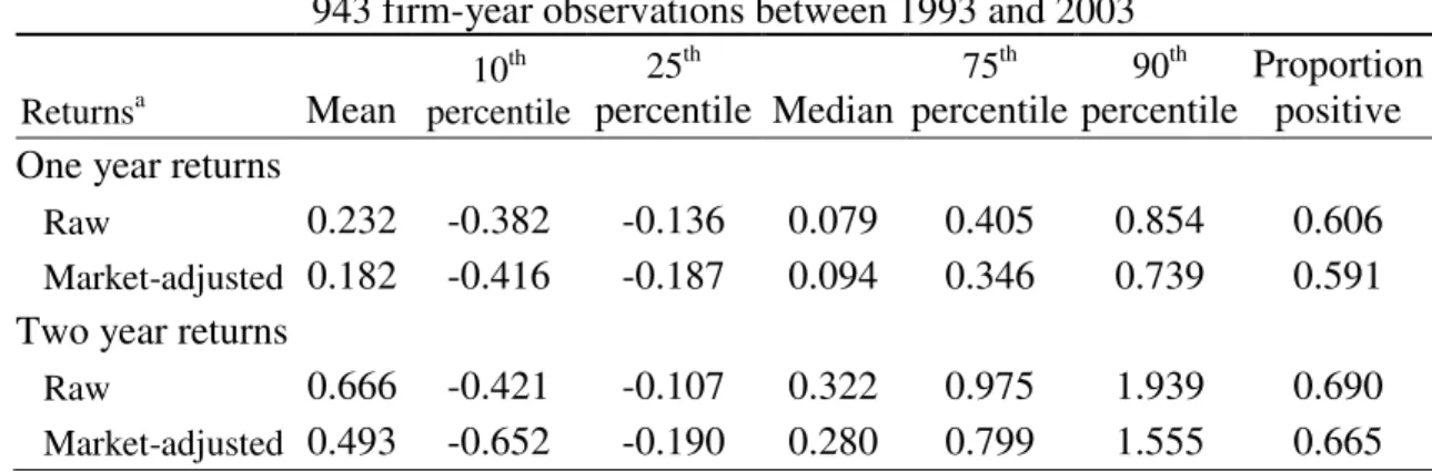
Table 2 provides descriptive statistics about one year and two year buy and hold returns for the higher B/M portfolio quintile. As in Fama and French (1992), Lakonishok, Shleifer, and Vishny (1994), and Piotroski (2000), the high B/M firms earn positive market-adjusted returns in the one year and two year analysis, but, although there is a high mean and median performance, a big proportion of the firms (40.9% and 33.5% in one year and two years windows, respectively) produce negative market-adjusted returns. The 10th percentile and the 25th percentile market-adjusted returns of the high B/M firms are also negative.

Therefore, as Piotroski (2000) explained, “any strategy that can eliminate the left-tail of the

return distribution (i.e., the negative return observations) will greatly improve the

portfolio's mean return performance.”

Table 1: Financial Characteristics of High Book-to-Market Firms

943 firm-year observations between 1993 and 2003

Variable1 Mean Median

Standard deviation

Proportion positive

MVE 308.239 24.850 1,410.409 n/a

ASSETS 3,755.996 125.800 30,930.763 n/a

B/M 2.152 1.695 1.995 n/a

ROA -0.001 0.012 0.127 0.639

ROA 0.049 -0.002 1.185 0.460

MARGIN 0.036 -0.004 2.250 0.442

CFO 0.036 0.048 0.357 0.799

LIQUID 0.149 -0.025 3.520 0.448

LEVER 0.091 -0.001 2.665 0.456

TURN -0.011 -0.001 0.367 0.485

ACCRUAL -0.036 -0.048 0.381 0.224

1

MVE = market value of equity at the end of fiscal year. Market value is calculated as the number of shares

outstanding times share price. In millions of euros.

(13)

B/M = book value of equity at the end of the fiscal year scaled by MVE.

ROA = net income before extraordinary items at the end of the fiscal year scaled by total assets at the

beginning of the fiscal year.

ΔROA= change in annual ROA. ΔROA is calculated as ROA at the end of the fiscal year less preceding year

ROA.

ΔMARGIN = change in the gross margin ratio between the fiscal year end and the preceding year. The gross margin ratio is defined as the gross margin divided by total sales.

CFO = cash flow from operations scaled by total assets at the beginning of the fiscal year.

ΔLIQUID = change in the current ratio between the fiscal year end and the preceding year. The current ratio is defined as total current assets divided by total current liabilities.

ΔLEVER = change in the assets ratio between the fiscal year end and the preceding year. The debt-to-assets ratio is defined as long-term debt scaled by total debt-to-assets at the beginning of the year.

ΔTURN = change in the asset turnover ratio between the fiscal year end and the preceding year. The asset turnover ratio is defined as net sales scaled by total assets.

ACCRUAL = net income before extraordinary items less cash flow from operations at the end of the fiscal year, scaled by total assets at the beginning of the fiscal year.

Table 2: Buy and Hold Returns from a High Book-to-Market Investment Strategy

943 firm-year observations between 1993 and 2003

Returnsa Mean

10th percentile

25th

percentile Median

75th percentile 90th percentile Proportion positive One year returns

Raw 0.232 -0.382 -0.136 0.079 0.405 0.854 0.606

Market-adjusted 0.182 -0.416 -0.187 0.094 0.346 0.739 0.591 Two year returns

Raw 0.666 -0.421 -0.107 0.322 0.975 1.939 0.690

Market-adjusted 0.493 -0.652 -0.190 0.280 0.799 1.555 0.665

a

One year (two years) raw return = 12 (24) month buy and hold return of the firm starting at the end of the fourth month after fiscal year end. Return compounding ends earlier of one year (two years) after return compounding started or the last month of Bloomberg Professional reported trading. If the firm delists, the delisting return is assumed zero. Market-adjusted return = buy and hold return less the value-weighted market return (all firms listed in Euronext stock markets with sufficient data) over the corresponding time period.

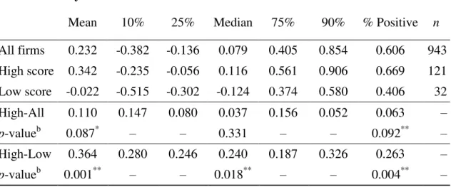
4.2. Piotroski Strategy

(14)

percentile, the 25th percentile, the median, the 75th percentile, and the 90th percentile returns of the higher score portfolio are higher for all observations than the corresponding higher B/M portfolio quintile. However, there is no statistical evidence of a difference in the medians. On average, a higher score firm returned 11.0% more than a higher B/M firm over the first year period. An investor that bought high score firms and sold low score firms would achieve a higher return: an average (median) one year raw return of 36.4% (24.0%). The proportion of positive results of higher score firms (66.9%) is bigger than the corresponding proportion of all higher B/M firms (60.6%) and lower score firms (40.6%). The results obtained form the one year raw return analysis (Panel A) can be extended to the one year market-adjusted return analysis (Panel B). On average, a high score firm achieve a one year market-adjusted return 9.2% higher than a high B/M firms and 32.4% higher than a low score firm.

The results from the two year analysis are not so clear. There is little statistical evidence that the higher score firms obtain a better result that the higher B/M firms over two year (Panel C), although it is obvious that a strategy that results in buying higher score firms and selling lower score firms registers an average and a median return improvement (81.2% and 44.3%, respectively) over the two year period. On the two year market-adjusted analysis (Panel D), there is no evidence that the return distribution is shifted to the right, since the 10th percentile, the 25th percentile, and the median returns of the higher score portfolio are lower than the corresponding observation for all higher B/M portfolio. However, the strategy that results in buying higher score firms and selling lower score firms keeps to show good results (72.5%).

Therefore, we find empirical support for the conclusions achieved by Piotroski (2000), now extended to Euronext-listed firms between 1993 and 2003. This seems to be particularly

true when we observe one year data: “Overall, it is clear that F_SCORE discriminates

(15)

Table 3: Buy and Hold Returns from Piotroski Strategy

This table summarises buy and hold returns achieved by a strategy based on financial signals developed by Piotroski (2000). F_SCORE is equal to the sum of nine individual binary signals (F_SCORE = F_ROA +

F_CFO + F_ΔROA + F_ACCRUAL + F_ΔLEVER + F_ΔLIQUID + EQ_OFFER + F_ΔMARGIN + F_ΔTURN). Each binary signal equals one (zero) if the underlying realisation is a good (bad) signal about future performance: F_ROA equals one if net income before extraordinary items at the end of the fiscal year scaled by total assets at the beginning of the fiscal year is positive, zero otherwise; F_CFO equals one if cash flow from operations scaled by total assets at the beginning of the fiscal year is positive, zero otherwise;

F_ΔROA equals one if the change in net income before extraordinary items at the end of the fiscal year scaled by total assets at the beginning of the fiscal year is positive, zero otherwise; F_ACCRUAL equals one if net income before extraordinary items less cash flow from operations at the end of the fiscal year, scaled by total

assets at the beginning of the fiscal year is negative, zero otherwise; F_ΔLEVER equals one if the change in

the debt-to-assets ratio (long-term debt scaled by total assets at the beginning of the year) between the fiscal year end and the preceding year is negative, zero otherwise; F_ΔLIQUID equals one if the change in the current ratio (total current assets divided by total current liabilities) between the fiscal year end and the preceding year is positive, zero otherwise; EQ_OFFER equals one if the firm did not issue common equity in

the preceding year, zero otherwise; F_ΔMARGIN equals one if the change in the gross margin ratio (gross

margin divided by total sales) between the fiscal year end and the preceding year is positive, zero otherwise; F_ΔTURN equals one if the change in the asset turnover ratio (net sales scaled by total assets) between the fiscal year end and the preceding year is positive, zero otherwise. The highest possible score for a firm is 9 while the lowest is 0. The high score portfolio consists of all firms with a composite score of 8 or 9. The low score portfolio consists of all firms with a score of 0 or 1. High-All measures the return difference between high score portfolio and all firms portfolio. High-Low measures the return difference between high score portfolio and low score portfolio.

Panel A: One year raw returnsa

Mean 10% 25% Median 75% 90% % Positive n

All firms 0.232 -0.382 -0.136 0.079 0.405 0.854 0.606 943 High score 0.342 -0.235 -0.056 0.116 0.561 0.906 0.669 121 Low score -0.022 -0.515 -0.302 -0.124 0.374 0.580 0.406 32 High-All 0.110 0.147 0.080 0.037 0.156 0.052 0.063 –

p-valueb 0.087* – – 0.331 – – 0.092** – High-Low 0.364 0.280 0.246 0.240 0.187 0.326 0.263 –

p-valueb 0.001** – – 0.018** – – 0.004** –

Panel B: One year market-adjusted returnsa

(16)

p-valueb 0.129 – – 0.169 – – 0.098* – High-Low 0.324 0.246 0.251 0.243 0.300 0.217 0.247 –

p-valueb 0.003** – – 0.018** – – 0.007** –

Panel C: Two years raw returnsa

All firms 0.666 -0.421 -0.107 0.322 0.975 1.939 0.690 943 High score 0.763 -0.239 -0.015 0.387 0.929 2.123 0.727 121 Low score -0.049 -0.727 -0.396 -0.056 0.191 0.534 0.438 32 High-All 0.097 0.182 0.092 0.065 -0.046 0.184 0.037 –

p-valueb 0.257 – – 0.332 – – 0.216 –

High-Low 0.812 0.488 0.381 0.443 0.738 1.589 0.289 –

p-valueb 0.000** – – 0.004** – – 0.002** –

Panel D: Two years market-adjusted returnsa

All firms 0.493 -0.652 -0.190 0.280 0.799 1.555 0.665 943 High score 0.553 -0.679 -0.231 0.244 0.882 1.788 0.661 121 Low score -0.172 -0.936 -0.639 -0.157 0.335 0.685 0.375 32 High-All 0.060 -0.027 -0.041 -0.036 0.083 0.233 -0.004 –

p-valueb 0.339 – – 0.403 – – 0.469 –

High-Low 0.725 0.257 0.408 0.401 0.547 1.103 0.286 –

p-valueb 0.000** – – 0.010** – – 0.002** –

a

b

P-values are from t-tests, except for the proportions that are based on a binomial test of proportions. * and **

(17)

4.3. Accruals Strategy

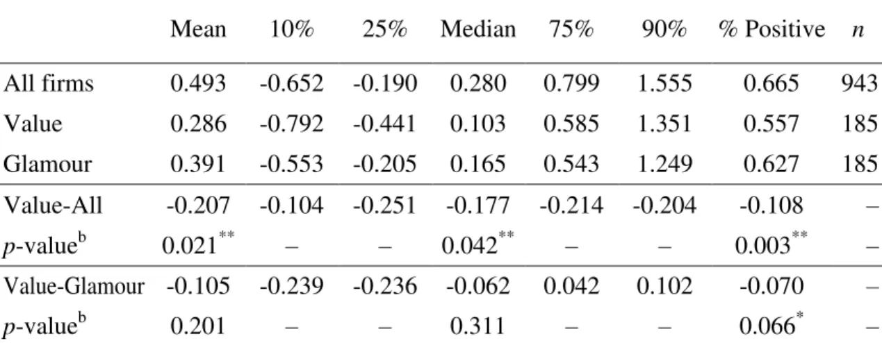
Table 4 displays the findings on buy and hold returns obtained with the investment strategy that uses accruals to segregate value firms (low accruals) from glamour firms (high accruals). The 10th percentile, the 25th percentile, and the median one year market adjusted returns (Panel B) of the value firms is lower than the corresponding observations for the higher B/M portfolio, which gives a clear signal that there is no evidence that this strategies shifts the return distribution to the right. Simultaneously, the 10th percentile and the 25th percentile returns are also lower than the corresponding percentile of the glamour firms. Thus, it seems that the accruals strategy just flattens the return distribution. The percentage of positive returns of the value firms is also inferior to the percentage of positive returns of the higher B/M firms and the glamour firms. There is also no evidence that the average rate of return difference between value firms (19.3%) and higher B/M firms (18.2%) differs from zero and the same applies to the average return difference between value firms and glamour firms (16.1%). All these differences present p-values that are far from 5% or 10%. Similar conclusions can be achieved from the one year raw returns (Panel A).

The two years raw returns (Panel C) and market-adjusted returns (Panel D) show even worse results for the accruals strategy. There is statistical evidence that value firms earned less than the higher B/M firms. The mean (median) difference of -20.8% (-19.2%) in raw returns and of -20.7% (-17.7%) in market-adjusted returns are statistically different from zero. There is also evidence that there are more higher B/M firms and glamour firms with positive raw and market-adjusted returns than value firms.

Overall, the results achieve by the accruals strategy do not give evidence supporting the conclusions presented by Bartov and Kim (2004). The findings do not show any evidence

that “genuine” value stocks outperform “genuine” glamour stocks or the market average, as

(18)

This table summarises buy and hold returns achieved by a strategy that uses accruals to separate “genuine” value firms and “genuine” glamour firms. Value portfolio consists of firms with accruals (net income before

extraordinary items less cash flow from operations, scaled by beginning of the year total assets) in the lowest

quintile. Glamour portfolio consists of firms with accruals in the highest quintile. Value-All measures the

return difference between value portfolio and all firms portfolio. Value-Glamour measures the return

difference between value portfolio and glamour portfolio.

All firms 0.232 -0.382 -0.136 0.079 0.405 0.854 0.606 943 Value 0.242 -0.507 -0.233 0.055 0.530 1.161 0.573 185 Glamour 0.210 -0.322 -0.133 0.085 0.325 0.708 0.605 185 Value-All 0.010 -0.125 -0.097 -0.024 0.125 0.307 -0.033 –

p-valueb 0.473 – – 0.355 – – 0.209 –

Value-Glamour 0.032 -0.185 -0.100 -0.030 0.205 0.453 -0.032 –

p-valueb 0.342 – – 0.355 – – 0.245 –

All firms 0.182 -0.416 -0.187 0.094 0.346 0.739 0.591 943 Value 0.193 -0.505 -0.248 0.085 0.407 0.962 0.562 185 Glamour 0.161 -0.337 -0.151 0.082 0.322 0.602 0.611 185 Value-All 0.011 -0.089 -0.061 -0.009 0.061 0.223 -0.029 –

p-valueb 0.429 – – 0.441 – – 0.239 –

Value-Glamour 0.032 -0.168 -0.097 0.003 0.085 0.360 -0.049 –

p-valueb 0.333 – – 0.483 – – 0.149 –

(19)

p-valueb 0.000** – – 0.037** – – 0.002** – Value-Glamour -0.104 -0.295 -0.275 -0.144 0.042 0.193 -0.157 –

p-valueb 0.211 – – 0.136 – – 0.000** –

Table 4: Buy and Hold Returns from Accruals Strategy –continued

All firms 0.493 -0.652 -0.190 0.280 0.799 1.555 0.665 943 Value 0.286 -0.792 -0.441 0.103 0.585 1.351 0.557 185 Glamour 0.391 -0.553 -0.205 0.165 0.543 1.249 0.627 185 Value-All -0.207 -0.104 -0.251 -0.177 -0.214 -0.204 -0.108 –

p-valueb 0.021** – – 0.042** – – 0.003** – Value-Glamour -0.105 -0.239 -0.236 -0.062 0.042 0.102 -0.070 –

p-valueb 0.201 – – 0.311 – – 0.066* –

a

b

represent differences statistically significant at a 10% and 5% levels, respectively.

4.3. Bankruptcy Probability Strategy

(20)

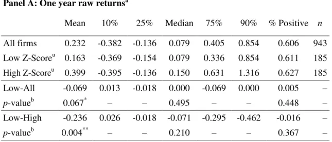
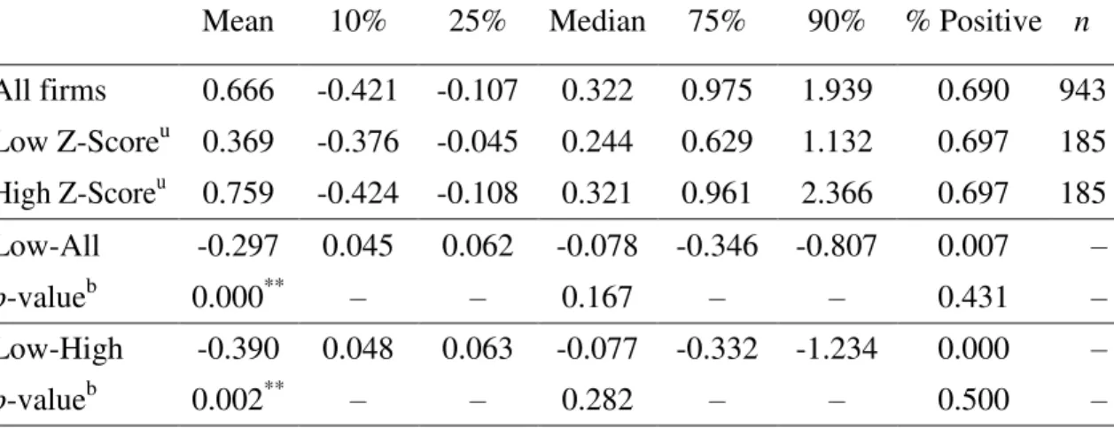
Table 6 presents findings when the updated measure, Hillegeist et al.'s (2004) Z-Scoreu, is used in the bankruptcy probability strategy. However, the results are even worse than the previous presented in Table 5. Panel B reports the one year market-adjusted returns. The 10th percentile, the 25th percentile, the median, the 75th percentile, the 90th percentile, and the average market-adjusted return of the low Z-Scoreu firms are lower than the corresponding higher B/M firms. So, instead of shifting the returns distribution to the right, the low Z-Scoreu strategy shifted the returns distribution to the left. The strategy that consists of buying low Z-Scoreu firms and selling high Z-Scoreu firms doesn't work too.

The average (median) return difference is negative, and the proportion of positive market-adjusted returns for lower Z-Scoreu firms is smaller than the corresponding indicator for higher Z-Scoreu firms. These conclusions can be extended almost with no changes to the one year raw returns (Panel A), two year raw returns (Panel B), and two year market-adjusted returns (Panel D) analysis.

Table 5: Buy and Hold Returns from Bankruptcy Probability Strategy (Z-Score)

This table summarises buy and hold returns achieved by a strategy that uses bankruptcy probability to

separate winner from losers. The Altman's (1968) ZScore is used as the probability of bankruptcy (Z =

-1.20X1– 1.40X2– 3.30X3– 0.60X4– 0.999X5 where X1 = working capital scaled by total assets, X2 =

retained earnings scaled by total assets, X3 = earnings before interest and taxes scaled by total assets, X4 =

market value of equity scaled by total debt, X5 = sales scaled by total assets; the signs of the original

coefficients have been changed so the Z-Score is increasing in the probability of bankruptcy; all coefficients

except X5 have been multiplied by 100, since Altman (1968) express each variable aside X5 as percentages

rather than in ratio form (see Hillegeist et al. (2004) for details)). Low Z-Score portfolio consists of firms that

are in the lowest Z-Score quintile. High Z-Score portfolio consists of firms that are in the highest Z-Score

quintile. All measures the return difference between low Z-Score portfolio and all firms portfolio.

Low-High measures the return difference between low Z-Score portfolio and high Z-Score portfolio.

(21)

All firms 0.232 -0.382 -0.136 0.079 0.405 0.854 0.606 943 Low Z-Score 0.222 -0.309 -0.116 0.098 0.468 0.854 0.632 185 High Z-Score 0.210 -0.505 -0.208 0.035 0.381 0.819 0.562 185 Low-All -0.010 0.073 0.020 0.019 0.063 0.000 0.026 –

p-valueb 0.420 – – 0.354 – – 0.252 –

Low-High 0.012 0.196 0.092 0.063 0.087 0.035 0.070 –

p-valueb 0.441 – – 0.205 – – 0.073* –

All firms 0.182 -0.416 -0.187 0.094 0.346 0.739 0.591 943 Low Z-Score 0.173 -0.350 -0.162 0.136 0.356 0.685 0.649 185 High Z-Score 0.161 -0.520 -0.250 0.023 0.332 0.890 0.503 185 Low-All -0.009 0.066 0.025 0.042 0.010 -0.054 0.058 –

p-valueb 0.417 – – 0.181 – – 0.075* – Low-High 0.012 0.170 0.088 0.113 0.024 -0.205 0.146 –

p-valueb 0.437 – – 0.059* – – 0.001** –

All firms 0.666 -0.421 -0.107 0.322 0.975 1.939 0.690 943 Low Z-Score 0.571 -0.325 -0.045 0.241 0.806 1.490 0.681 185 High Z-Score 0.518 -0.622 -0.326 0.162 0.627 1.566 0.562 185 Low-All -0.095 0.096 0.062 -0.081 -0.169 -0.449 -0.009 –

p-valueb 0.217 – – 0.253 – – 0.408 –

Low-High 0.053 0.297 0.281 0.079 0.179 -0.076 0.119 –

p-valueb 0.384 – – 0.331 – – 0.008** –

(22)

All firms 0.493 -0.652 -0.190 0.280 0.799 1.555 0.665 943 Low Z-Score 0.400 -0.662 -0.232 0.206 0.648 1.132 0.643 185 High Z-Score 0.346 -0.855 -0.507 0.040 0.538 1.387 0.535 185 Low-All -0.093 -0.010 -0.042 -0.074 -0.151 -0.423 -0.022 –

p-valueb 0.214 – – 0.266 – – 0.294 –

Low-High 0.054 0.193 0.275 0.166 0.110 -0.255 0.108 –

p-valueb 0.381 – – 0.175 – – 0.013** –

a

b

represent differences statistically significant at a 10% and 5% levels, respectively.

4.5. Graphical Analysis

Figure 1 gives pictorial evidence about the previous inferences on the one year raw return analysis. Comparing the higher B/M firms returns distribution (Panel A) with the higher score firms returns distribution achieved with the Piotroski (2000) strategy (Panel B), it is clear that F_SCORE shifts the distribution to the right. The right tail is heavier while parts from the left tail vanished. Actually, there is no observation in the high score with a one year return smaller than -88.1%.

(23)

Table 6: Buy and Hold Returns from Bankruptcy Probability Strategy (Z-Scoreu)

This table summarises buy and hold returns achieved by a strategy that uses bankruptcy probability to

separate winner from losers. The Z-Score updated by Hillegeist et al. (2004) is used as the probability of

bankruptcy (Zu = -0.08X1 + 0.04X2– 0.10X3– 0.22X4 + 0.06X5– 4.34 where X1 = working capital scaled by

total assets, X2 = retained earnings scaled by total assets, X3 = earnings before interest and taxes scaled by

total assets, X4 = market value of equity scaled by total debt, X5 = sales scaled by total assets). Low Z-Scoreu

portfolio consists of firms that are in the lowest Z-Scoreu quintile. High Z- Scoreu portfolio consists of firms

that are in the highest Z-Scoreu quintile. Low-All measures the return difference between low Z- Scoreu

portfolio and all firms portfolio. Low-High measures the return difference between low Z- Scoreu portfolio

and high Z- Scoreu portfolio.

All firms 0.232 -0.382 -0.136 0.079 0.405 0.854 0.606 943 Low Z-Scoreu 0.163 -0.369 -0.154 0.079 0.336 0.854 0.611 185 High Z-Scoreu 0.399 -0.395 -0.136 0.150 0.631 1.316 0.627 185 Low-All -0.069 0.013 -0.018 0.000 -0.069 0.000 0.005 –

p-valueb 0.067* – – 0.495 – – 0.448 – Low-High -0.236 0.026 -0.018 -0.071 -0.295 -0.462 -0.016 –

p-valueb 0.004** – – 0.210 – – 0.367 –

All firms 0.182 -0.416 -0.187 0.094 0.346 0.739 0.591 943 Low Z-Scoreu 0.114 -0.430 -0.201 0.093 0.308 0.731 0.600 185 High Z-Scoreu 0.350 -0.504 -0.136 0.216 0.511 1.189 0.654 185 Low-All -0.068 -0.014 -0.014 -0.001 -0.038 -0.008 0.009 –

p-valueb 0.054* – – 0.486 – – 0.408 – Low-High -0.236 0.074 -0.065 -0.123 -0.203 -0.458 -0.054 –

p-valueb 0.003** – – 0.072* – – 0.128 –

(24)

All firms 0.666 -0.421 -0.107 0.322 0.975 1.939 0.690 943 Low Z-Scoreu 0.369 -0.376 -0.045 0.244 0.629 1.132 0.697 185 High Z-Scoreu 0.759 -0.424 -0.108 0.321 0.961 2.366 0.697 185 Low-All -0.297 0.045 0.062 -0.078 -0.346 -0.807 0.007 –

p-valueb 0.000** – – 0.167 – – 0.431 – Low-High -0.390 0.048 0.063 -0.077 -0.332 -1.234 0.000 –

p-valueb 0.002** – – 0.282 – – 0.500 –

All firms 0.493 -0.652 -0.190 0.280 0.799 1.555 0.665 943 Low Z-Scoreu 0.197 -0.714 -0.242 0.134 0.498 0.995 0.600 185 High Z-Scoreu 0.588 -0.669 -0.187 0.297 0.868 2.071 0.065 185 Low-All -0.296 -0.062 -0.052 -0.146 -0.301 -0.560 -0.065 –

p-valueb 0.000** – – 0.035** – – 0.052* – Low-High -0.391 -0.045 -0.055 -0.163 -0.370 -1.076 -0.065 –

p-valueb 0.001** – – 0.105 – – 0.087* –

a

One year (two years) raw return = 12 (24) month buy and hold return of the firm starting at the end of the fourth month after fiscal year end. Return compounding ends earlier of one year (two years) after return compounding started or the last month of Bloomberg

Professional reported trading. If the firm delists, the delisting return is assumed zero.

Market-adjusted return = buy and hold return less the value-weighted market return (all firms listed in Euronext stock markets with sufficient data) over the corresponding time period.

b

P-values are from t-tests, except for the proportions that are based on a binomial test of proportions.

Figure 1: One Year Raw Return Histograms Between 1993 and 2003

(25)

Panel B: Higher score firms (Piotroski strategy)

Panel C: Value firms (accruals strategy)

Panel D: Lower Z-Score (bankruptcy probability strategy)

Panel E: Lower Z-Scoreu (bankruptcy probability strategy)

5. CONCLUSIONS

(26)

to select firms with good financial prospects. The third strategy selects low bankruptcy probability firms from within the higher B/M portfolio quintile.

Only one of the three strategies in this article resisted testing. It was shown that the annual mean return achieve by a high B/M firm is increased by 9.2% using F_SCORE developed by Piotroski (2000) when applied to a sample of European stocks during an 11 year period. A strategy that consists of buying potential winner and selling potential losers achieved a 32.4% annual return between 1993 and 2003 when applied to a set of 943 firms elected from the top B/M ratio quintile of a sample of 4,715 firms listed in the four Euronext markets. Furthermore, there is a clear evidence that the entire high B/M firms return distribution is shifted to the right when the high score screen is applied. These findings

allow an extension of Piotroski (2000) conclusions: “the results convincingly demonstrate

that investors can use relevant historical information to eliminate firms with poor future prospects from a generic high B/M portfolio.” The return increase of 9.2% achieve using F_SCORE and the annual return of 32.4% obtained when buying potential winners and selling potential losers are bigger than the corresponding returns presented by Piotroski (2000) for the U.S. stock market (7.4% and 23.5%, respectively).

This study suffers from a potential survivorship bias, even though many delisted firms were detected during data collecting. Another limitation of this paper is the potential inexistence of the assumed risk homogeneity in the higher B/M portfolio quintile. A possible future research can extend these conclusions using abnormal returns instead of market-adjusted returns, correcting for a potential heterogeneity of risk levels within the higher B/M portfolio quintile.

8. REFERENCES

Ali, A., Hwangb, L. and Trombley, M. (2003), Arbitrage Risk and the Book-to-Market Anomaly, Journal of Financial Economics, 69, pp. 355-373.

Altman, E. (1968), Financial Ratios, Discriminant Analysis, and the Prediction of Corporate Bankruptcy, Journal of Finance, 23, pp. 589-609.

(27)

Market Efficiency and Serial Correlation of Returns, Journal of Financial Economics, 25, pp. 51-74. Bartov, E. and Kim, M. (2004), Risk, Mispricing, and Value Investing, Review of Quantitative Finance and Accounting, 23, pp. 353-376.

Basu, S. (1977), Investment Performance of Common Stocks in Relation to their Price-Earnings Ratios: A Test of the Efficient Market Hypothesis, Journal of Finance, 32, pp. 663-682.

Bernard, V. and Thomas, J. (1989), Post-Earnings Announcement Drift: Delayed Price Response or Risk Premium?, Journal of Accounting Research, 27, pp. 1-36.

Bernard, V. and Thomas, J. (1990), Evidence that Stock Prices do not Fully Reflect the Implications of Current Earnings for Future Earnings, Journal of Accounting and Economics, 13, pp. 305-340.

Chan, K. (1988), On the Contrarian Investment Strategy, Journal of Business, 61, pp. 147-163. Chan, L., Hamao, Y., and Lakonishok, J. (1991), Fundamentals and Stock Returns in Japan, Journal of Finance, 46, pp. 1739-1789.

Chen, N. and Zhang, F. (1998), Risk and Return of Value Stocks, Journal of Business, 71, pp. 501-535.

Chopra, N., Lakonishok, J., and Ritter, J. (1992), Measuring Abnormal Performance: Do Stocks Overreact?, Journal of Financial Economics, 31, pp. 235-268.

De Bondt, W. and Thaler, R. (1985), Does the Stock Market Overreact?, Journal of Finance, 40, pp. 793-805.

De Bondt, W. and Thaler, R. (1987), Further Evidence on Investor Overreaction and Stock Market Seasonality, Journal of Finance, 42, pp. 557-581.

Dichev, I. (1998), Is the Risk of Bankruptcy a Systematic Risk?, Journal of Finance, 53, pp. 1131-1147.

Dreman, D. (1977) Psychology and the Stock Market: Why the Pros Go Wrong and How to Profit, New York: Warner Books.

Fama, E. and French, K. (1992), The Cross-Section of Expected Stock Returns, Journal of Finance, 47, pp. 427-465.

Fama, E. and French, K. (1995), Size and Book-to-Market Factors in Earnings and Returns, Journal of Finance, 50, pp. 131-155.

Fama, E. and French, K. (1998), Value Versus Growth: The International Evidence, Journal of Finance, 53, pp. 1975-1999.

Foster, G., Olsen, C., and Shevlin, T. (1984), Earnings Releases, Anomalies, and the Behavior of Securities, The Accounting Review, 59, pp. 574-603.

Frankel, R. and Lee, R. (1998), Accounting Valuation, Market Expectation, and Cross-Sectional Stock Returns, Journal of Accounting and Economics, 25, pp. 283-319.

Graham, B. and Dodd, D. (1934), Security Analysis, New York: McGraw-Hill.

Hayes, R. (1998), The Impact of Trading Commission Incentives on Analysts' Stock Coverage Decisions and Earnings Forecasts, Journal of Accounting Research, 36, pp. 299-320.

Hillegeist, S., Keating, E., Cram, D., and Lundsted, K. (2004), Assessing the Probability of Bankruptcy, Review of Accounting Studies, 9, pp. 5-34.

Ikenberry, D., Lakonishok, J., and Vermaelen, T. (1995), Market Underreaction to Open Market Share Repurchases, Journal of Financial Economics, 39, pp. 181-208.

Jaffe, J., Keim, D., and Westerfield, R. (1989), Earnings Yields, Market Values, and Stock Returns, Journal of Finance, 44, pp. 135-148.

La Porta, R., Lakonishok, J., Shleifer, A., and Vishny, R. (1997), Good News for Value Stocks: Further Evidence on Market Efficiency, Journal of Finance, 52, pp. 859-874.

Lakonishok, J., Shleifer, A., and Vishny, R. (1994), Contrarian Investment, Extrapolation, and Risk, Journal of Finance, 49, pp. 1541-1578.

(28)

Michaely, R., Thaler, R., and Womack, K. (1995), Price Reactions to Dividends Initiations and Omissions: Overreaction or Drift?, Journal of Finance, 50, pp. 573-608.

Piotroski, J. (2000), Value Investing: The Use of Historical Financial Statement Information to Separate Winners from Losers, Journal of Accounting Research, 38, pp. 1-41.

Rosenberg, B., Reid, K., and Lanstein, R. (1984), Persuasive Evidence of Market Inefficiency, Journal of Portfolio Management, 11, pp. 9-17.

Shleifer, A. and Vishny, R. (1997), The Limits of Arbitrage, Journal of Finance, 52, pp. 35-55. Skinner, D. and Sloan, R. (2002), Earnings Surprises, Growth Expectations, and Stock Returns, or, Don’t Let an Earnings Torpedo Sink Your Portfolio, Review of Accounting Studies, 7, pp. 289-312.

Sloan, R. (1996), Do Stock Prices Fully Reflect Information in Accruals and Cash Flows about Future Earnings?, The Accounting Review, 71, pp. 289-316.