Term Structure Models with Shot-noise Effects

Term Structure Models with Shot-noise Effects

W ORKI N G PAPER N .3 / 2 0 0 7

July 2007

Abst r a ct

This work proposes t erm st ruct ure m odels consist ing of t w o part s: a part which can be represent ed in exponent ial quadrat ic form and a shot noise part . These t erm st ruct ure m odels allow for explicit expressions of various derivat ives. I n part icular, t hey are very w ell suit ed for credit risk m odels.

The goal of t he paper is t wofold. First , a num ber of key building blocks useful in t erm st ruct ure m odelling are derived in closed- form . Second, t hese building blocks are applied t o single and port folio credit risk. This approach generalizes Duffie & Gârleanu ( 2001) and is able t o produce realist ic default correlat ion and default clust ering. We conclude w it h a specific m odel w here all key building blocks are com put ed explicit ly.

Ke y W or ds: Term St ruct ure Models, Quadrat ic Term St ruct ure Models, Shot - noise processes.

JEL Cla ssifica t ion : C15,C12, G13, G33

D e pa r t m e n t of M a n a ge m e n t W or k ing pa pe r Se r ie s

Raquel M. Gaspar Advance Reseach Cent er I SEG, Technical Universit y of Lisbon

e- m ail: Rm gaspar@iseg.ut l.pt

Thorst en Schm idt Depart m ent of Mat hem at ics

Universit y of Leipzig

Term Structure Models with Shot Noise Effects

Raquel M. Gaspar

and Thorsten Schmidt

July 2007

Abstract

This work proposes term structure models consisting of two parts: a part which can be represented in exponential quadratic form and a shot noise part. These term structure models allow for explicit expressions of various derivatives. In particular, they are very well suited for portfolio credit risk models and for the pricing of CDOs. The goal of the paper is twofold. First, a number of key building blocks useful in term structure modelling are derived in closed-form. Second, these building blocks are ap-plied to single and portfolio credit risk. This approach generalizes Duffie and Gˆarleanu (2001) and is able to produce realistic default correlation and default clustering. We conclude with a specific model where all key building blocks are computed explicitly.

1

Introduction

The aim of this paper is to put forth a new class of term structure models, which general-izes affine and jump-diffusion models and still allows for closed form solutions to prices of numerous derivatives. This class is particularly suited to applications in single and portfolio credit risk.

Using the framework of intensity-based models3

the proposed class combines the concept of general quadratic term structure (GQTS) models put forth in Gaspar (2004) with a special type of jump-processes, called shot noise processes. The obtained results show that shot noise processes can be paired with any other, independent class of processes and we choose GQTS for the following reasons: First, the considered factors need not to be Gaussian as, e.g., is the case in Chen, Filipovi´c, and Poor (2004). Second, they include affine term structures as a special case. Third, the proposed framework naturally allows for negative correlation of interest rates and default intensities, which is a rather delicate issue in affine models, as pointed out in Chapters 5.8.2 and 5.8.3 of Lando (2004). Fourth, the quadratic class is the largest polynomial class which can be considered without introducing arbitrage opportunities (see Filipovi´c (2002) or Gaspar (2004)).

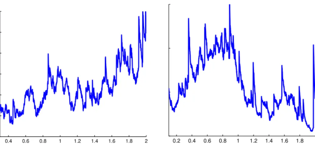
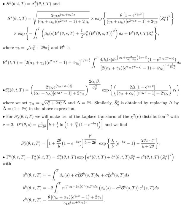
On the other side, considering shot noise processes includes jump-diffusion models, like Duffie and Gˆarleanu (2001), as special cases but allows for greater flexibility. In fact, we show how to add several constant intensity jump processes with arbitrary decay rates to any given quadratic diffusion component. Moreover, shot noise patterns are often evident from market data (see Figure 1 for typical patterns of credit default swap (CDS) spreads and Figure 2 for a simulated path of a model of the proposed class). As argued in Mortensen (2006), common jumps in intensities are an efficient way to reproduce observed correlation smiles in the market. In particular, our setup allows to overcome a difficulty in Duffie and Gˆarleanu

1

Advance Research Center, ISEG, Technical University of Lisbon, Rua Miguel Lupi 20, 1249-078 Lisboa, PORTUGAL. Email: Rmgaspar@iseg.utl.pt

2

Augustusplatz 10/11, 04109 Leipzig, GERMANY. Email: thorsten.schmidt@math.uni-leipzig.de 3

10/8/05 12/8/05 2/8/06 4/8/06 6/5/06 500

600 700 800 900 1000 1100 1200 1300 1400

8/8/05 10/8/05 12/8/05 2/8/06 4/8/06 6/5/06 500

550 600 650 700 750 800 850 900 950 1000

Figure 1: 5-year credit spreads of General Motors (left) and Ford (right). The quoted spread is in basis points and is shown from August 8th, 2005 to June 5th, 2006. Data-source: Bloomberg.

(2001), as in the proposed class the mean-reversion speed of the diffusive and the jump part can be adjusted separately. Finally, for the application to portfolio credit risk the shot noise component allows to obtain a suitable dynamic dependence structure and produces clustered defaults. Needless to say, capturing dynamic dependencies is one of the most important points for modeling portfolio credit derivatives as collateralized debt obligations (CDOs) or First-to-default swaps. In addition, a subclass of the proposed model allows for separate calibration to single name and portfolio credit risk instruments, a useful property in the pricing of portfolio products, see Proposition 4.3. Phrased in market language, the marginal default distribution can be fixed first and the correlation between defaults can then be independently adjusted. For other applications of shot noise processes in finance see, e.g., Altmann, Schmidt, and Stute (2007) and Dassios and Jang (2003).

A recent branch of affine models allows for direct contagion modelling, i.e. a default of one firm has an immediate impact on the default intensity of the other firms. Pioneered by Davis and Lo (2001), there are a number of approaches considering on this topic. We refer to Collin-Dufresne, Goldstein, and Hugonnier (2004), Frey, Prosdocimi, and Runggaldier (2007) and Frey and Runggaldier (2006). The model proposed in this paper excludes this kind of direct contagion. Nonetheless, contagion effects are captured via the shot-noise part as explained above. Being technically simpler, and still capturing typical default correlations, the chosen approach seems to be very suitable for practical applications.

The main goals of this paper are:

• To use GQTS and shot noise processes to model default risk.

• To get explicit solutions (up to ODE systems solving) for all crucial expectations, here called thecredit risk building blocks.

• To use these building blocks to obtain key ingredients in credit risk, such as probabil-ities of default and prices of risk-free and defaultable bonds, CDSs, etc.

The paper is organized as follows: in Section 2 we briefly review the GQTS. In Section 3 we present the model and the key building blocks are derived. Section 4 shows the use of the key building blocks providing several applications to the pricing of credit risk. In Section 5 we consider a three-factor model and provide all necessary expressions explicitly.

2

Risk-free bond market

For the risk-free bond market we use the GQTS setup studied in Gaspar (2004). This setup assumes as given factors described by aRm_{-valued stochastic process (Z}

t)t≥0 whose dynamics, under the risk-neutral martingale measureQ, are of a special form. Furthermore, it assumes that the risk-free rate of interestris quadratic on those factors.

Assumption 2.1. W is ann-dimensional standard Brownian motion andZ is the unique strong solution of

dZt=α(t, Zt)dt+σ(t, Zt)dWt.

Hereα:R+×Rm7→Rm andσ:R+×Rm7→Rn×n are such that

α(t, z) =d(t) +E(t)z (1)

σ(t, z)σ⊤_{(t, z) =k0(t) +}

m

X

i=1

ki(t)zi+ m

X

i,j=1

zigij(t)zj (2)

with smooth functions d: R+ 7→ Rm, E, k0, ki and gij, i, j= 1,· · ·, m map R+ to Rm×m. Moreover, the risk-free short rate(rt)t≥0 is given by

r(t, Zt) =Zt⊤Q(t)Zt+g⊤(t)Zt+f(t). (3)

Q, gandf are smooth, mappingR+ toRm×m,Rm andR. Q(t)is symmetric4 for allt.

We classify factors based on their impact on the drift, volatility or the short rate.

Definition 2.2. (Classification of risk-free factors)

• Ziis arisk-free quadratic-factorif it satisfiesat least oneof the following requirements:

(i) it has a quadratic impact on the short rate, i.e., there existstsuch thatQi(t)6= 0; (ii) it has a quadratic impact onσσ⊤_{, i.e., there existj and tsuch thatg}

ij(t)6= 0; (iii) it affects the drift term of the factors satisfying (i) or (ii), i.e., for some Zj

satisfying (i) or (ii) we haveEji(t)6= 0, at least for somet.

• Zi is a risk-free linear-factor, if it does not satisfy any of (i)-(iii).

We write symbolicallyZi∈Z(q), ifZiis a risk-free quadratic factor andZi∈Z(l)otherwise.

Finally, based upon on the factor’s classification, it is possible to derive under what con-ditions we will have a quadratic term structure of (zero-coupon) risk-free bond prices. To explicitly get the term structure we will always have to solve what we will here define as basic ODE system.

4_{The symmetry assumption is not restrictive. Any non-symmetric quadratic form can be rewritten in an}

Definition 2.3. (Basic ODE System) Denote T := {(t, T) ∈ R2 : 0 ≤ t ≤ T} and consider functionsA, B and C on T with values in R, Rm and Rm×m, respectively. For functionsφ1 andφ2, φ3 onR+ with values in R, Rm and Rm×m, respectively, we say that (A, B, C, φ1, φ2, φ3) solves thebasic ODE system if

∂A ∂t +d

⊤_(t)B+1

2B

⊤_{k0(t)B+ tr}

{Ck0(t)}=φ1(t)

∂B ∂t +E

⊤_{(t)B+ 2Cd(t) +}1

2B˜

⊤_{K(t)B+ 2Ck0(t)B=φ2(t)}

∂C

∂t +CE(t) +E

⊤_{(t)C+ 2Ck0(t)C+}1

2B˜

⊤_{G(t) ˜B=φ3(t)}

subject to the boundary conditions A(T, T) = 0, B(T, T) = 0, C(T, T) = 0. A, B and C should always be evaluated at (t, T). E,d, k0, are the functions from the above definitions (recall (1)-(2)) while

˜ B:=



   

B 0 · · · 0

0 B · · · 0

..

. . ..

0 · · · 0 B



   

, K(t) = 

 

k1(t) .. . km(t)





, G(t) = 

 

g11(t) · · · g1m(t)

..

. . .. ...

gm1(t) · · · gmm(t)



 , (4)

where we have ˜B, K(t)∈Rm2×mandG(t)∈Rm2×m2.

The main result on risk-free bond prices’ term structure is the following.5

Result 2.4. (Gaspar) Suppose that Assumption 2.1 holds and factors in Z have been reordered asZ= (Z(q)_{, Z}(l)₎⊤_{. If fork}

i andgij in (2) we have that

ki=





0 0

0 k_i(ll) 

∀ i and gij =





0 0

0 gij(ll)



 ∀i, j s.t. Zi, Zj ∈Z(q),

then the term structure of risk-free zero-coupon bond prices is given by

p(t, T) = exphA(t, T) +B⊤(t, T)Zt+Zt⊤C(t, T)Zt

i

where(A, B, C, f, g, Q) solves the basic ODE system from Definition 2.3. Recall that f, g andQwere given in Equation (3). Moreover,C has only quadratic factors.

3

Defaultable bond market

In this section we present the defaultable bond market. To this, we use the well-known framework of doubly stochastic random times. For an introduction to this topic we refer to McNeil, Frey, and Embrechts (2005) or Bielecki and Rutkowski (2002).

3.1

Default events

The default intensity is modelled as a linear combination of GQTS and shot noise processes. Throughout we assume Assumption 2.1 is in force6_.

Assumption 3.1. (Default Events and Filtrations)

Consider a standard Poisson process N˜ with intensity l7_{. Denote the jumping times of N˜} byτ˜1,τ˜2, . . .. The processesη,J andµ are strictly positive and follow

ηt = Zt⊤Q(t)Zt+g⊤(t)Zt+f(t) (5)

Jt =

X

˜ τi≤t

Yih(t−τ˜i), (6)

µt = ηt+Jt. Here Q,g and f are smooth functions mapping R+ to Rm×m, Rm and R, respectively. Q(t)is symmetric for allt. Yi, i= 1,2, . . . are i.i.d., independent of W andN˜ andhis a differentiable function onR+. The default time τ is a doubly stochastic random time with intensity(µt)t≥0.

J is called ashot noise process.

Throughout, denote by FX _{the natural filtration generated by a generic process X. We} classify the market information according to the following filtrations: FW _the informa-tion about the diffusion factors; FJ _{the information about the jump factors; the} filtra-tion Ht := σ

¡

1{τ >s}: 0≤s≤t

¢

, information on the default state; Ft := FtW ∨ FtJ =

σ(Zs, Js: 0≤s≤t), information about all market factors and Gt := Ft∨ Ht, the total information. For future convenience, we also define

H(x) := Z x

0

h(u)du, D(θ, x) := Z 1

0

ϕ[θH(x(1−u))]du (7)

J(t, T) := X ˜ τi≤t

Yih(T−τ˜i), J˜(t, T) =

X

˜ τi≤t

YiH(T−τ˜i), (8)

whereϕ(θ) :=E(exp(θY1)). Note thatJ(t, t) =Jtand we set ˜Jt:= ˜J(t, t).

Intuitively, the modeling of a quadratic component and a shot noise component leads to the intensity being driven by a predictable component (the quadratic part) as well as by an unpredictable component (the jump part). We note that bothη andJ are assumed to be strictly positive. This assumption is needed becauseµis supposed to be an intensity. This point distinguishes classical interest rate models from reduced-form credit risk models in that in contrast to interest rates, negative intensities show a model inconsistency. Unfortunately, this is the case for some affine intensity models. Even if, through parameter restrictions, positiveness can be guaranteed, this usually comes at the cost of a loss in flexibility. In Proposition 3.3 we show that in our setting positivity can be guaranteed under very mild assumptions. This is a crucial point in favor of quadratic processes over affine processes for modelling the predictable part of the intensity.

For the shot noise part, Figure 2 shows a possible realization ofJ underh(x) = exp(−bx). Note that for realistic modeling the decay factorbof the shot noise part is by far larger than the mean reversion speedκ, which is a key improvement over affine jump-diffusions, as used for example in Duffie and Gˆarleanu (2001).

2.2, we give anintensity classification of factors.

6_{Taking the same factorsZas for the risk-free process is no loss of generality.}

0.4 0.6 0.8 1 1.2 1.4 1.6 1.8 2 0.2 0.4 0.6 0.8 1 1.2 1.4 1.6 1.8

Figure 2: Simulation of J withh(x) = e−bx _{for b = 30(right) andb = 50(left), χ}2

2

-distributedYi with additional quadratic part. The quadratic part is CIR with with mean

reversion speedκ= 0.5, mean reversion levelθ= 1and volatilityσ= 2.

Definition 3.2. (Classification of intensity factors). We callZianintensity quadratic-factor if it satisfies (ii) or (iii) in Definition 2.2 or it has a quadratic impact onη, i.e. ∃t≥0 such thatQi(t)6= 0; We callZianintensity linear-factorif it does not satisfy either of these. We writeZi∈Zη(q), Zη(l)for the quadratic and linear intensity factors, respectively8.

The next proposition gives a condition guaranteeing non-negativity of the default intensity.

Proposition 3.3. Assume that for allt≥0,Q(qq)(t)is symmetric and nonnegative definite,

g(q)(t)lies in the subspace spanned by the columns ofQ(qq)(t)andf(t)≥0. Denote byZη(q∗)(t)

the solution ofQ(qq)(t)Zη(q)(t) =−1₂g(q)(t). Then η is non-negative, if the following holds9:

(i) forZi∈Zη(l), either Zi≥0 andgi(l)≥0 orZi≤0andg(il)≤0,

(ii) for allt≥0, 1 2g

(q)⊤_Z(q)

η∗(t) +f(t)≥0.

Proof. Let Zi be a linear factor, say Zi ∈ Zη(l). As f ≥0, the result follows trivially from the fact that, by Definition 3.2,Q(ll)(t) = 0 and Q(lq)(t) =¡Q(ql)(t)¢⊤ = 0 for allt. For a quadratic factor we need to studyQ(qq) _andg(q)_{. Since Q}(qq) _{is nonnegative definite, Z}(q)

∗

is the minimum of the polynomialZη(q)⊤Q(qq)Zη(q)+g(q)⊤Zη(q), and hence 1₂g(q)⊤Zη(q∗)+f≥0

guarantees nonnegativity. ¥

Typically, shot-noise processes are not Markovian. Still, from a computational point of view Markovianity could be preferable. We provide a clear classification.

Proposition 3.4. Assume that for all x ∈ [0,∞) h(x) 6= 0. Then the process (Jt)t≥0 is Markovian, if and only ifhis of the form h(t) =ae−bt. In this case (J, η)is Markovian.

Proof. It is clear that for b= 0 the process is Markovian, so we need to consider the case wherehis not constant. Assume w.l.o.g. that h(0) = 1. To show thatJ is Markovian we compute the conditional expectation. Considers < tand recallFJ

t :=σ{Js:s≤t}. Then

8_{We use the symbolic notation ¯Z}(q)_=Z(q)_∪Z(q)

η and ¯Z(l)=Z(l)∩Zη(l), whenever the factors must be

ordered according toboth_{their impact onrand onη.}

9_{Here we use the following symbolic notation forgandQ: g=}

µ

g(q)

g(l)

¶ ,Q=

µ

Q(qq) _Q(ql)

Q(lq) _Q(ll)

EQ£Jt|FsJ

¤ =

˜ Ns

X

i=1

Yih(t−τ˜i) +EQ

·Nt˜−Ns˜ + ˜Ns

X

i= ˜Ns+1

Yih(t−τ˜i)

¯ ¯ ¯FsJ

¸

. (9)

As ˜N has independent increments and the Yi are identically distributed, we obtain

EQhPNt˜−Ns˜ +j

i=j+1 Yih(t−τ˜i)

¯ ¯N˜s=j

i

=EQhPNt˜−s

i=1 Yih(t−τ˜i)

i

=:f(s, t).

Hence (9) =PNs_i˜₌₁Yih(t−τ˜i)+f(s, t). Asf(s, t) is deterministic, necessary for Markovianity is that there exists a (measurable) functionF(t, s, x), such that

P_Ns˜

i=1Yih(t−τ˜i) =F(t, s, Js) =F

³

t, s,PNs_i˜₌₁Yih(s−˜τi)

´

. (10)

Note that each Yi is independent of all the other appearing terms. We will exploit this property to analyze the behavior ofF. Fixj and consider (10) on the set{N˜t> j}. Taking the conditional expectation of (10) w.r.t.Yj =ygives

EQ³_yh(t

−τ˜j) +P

˜ Ns

i=1,i6=jYih(t−τ˜i)

´

=EQ³_F¡_{t, s, yh(s}

−τ˜j) +P

˜ Ns

i=1,i6=jYih(s−˜τi)¢´.

Deriving w.r.t.y shows that

EQ¡_h(t

−τ˜j)¢=EQ

· Fx

³

t, s, yh(s−τ˜j) +P ˜ Ns

i=1,i6=jYih(s−τ˜i)

´

h(s−τ˜j)

¸ ,

where we denoted the partial derivative ofF w.r.t.xbyFx. As the l.h.s. does not depend ony, Fx(t, s, x) must be constant in x, and thusF must be of the form α(t, s) +β(t, s)x. Examining F on the set {N˜t = 0}, we see that α(t, s) must necessarily be 0. In the next step we determineβ. From Equation (10) we obtain, for anyi,h(t−τ˜i) =β(s, t)h(s−τ˜i). Hence, β(s, t) = h(t−y)/h(s−y) for any y ≥ 0, and so b(s, t) = h(t)/h(s). From this we have h(t−y)/h(s−y) = h(t)/h(s), for all t, s, y ≥ 0. By letting s = y we obtain that h(t −y) = h(0)h(t)/h(y) and so h(t+y) = h(t)h(y)/h(0). We conclude h′_{(y) =}

h′_{(0)h(y)/h(0). Thereforehis of the formae}−by_. For the converse, note that for h(y) = e−by_, PNt˜

i=1Yih(t−τ˜i) = h(t)P ˜ Nt

i=1Yih(−τ˜i), and henceJ is Markovian. Finally, independence ofJ andηimplies Markovianity of (J, η). ¥

It is clear that Markovianity ofµ itself only holds in very special cases. One well-known case is, whenη is affine, has mean reversion speedb andh(t) = exp(−bt).

Remark 3.5. In the Markovian case the terms in (7)-(8) simplify considerably. Forh(x) = e−bx _{we have thatH(x) =} 1

b

¡

1−e−bx¢_{. Thus,H(T−τ˜}

i)−H(t−τ˜i) =h(t−τ˜i)H(T−t), as well asJ˜t−J˜(t, T) =−H(T−t)Jt.

3.2

Building blocks

In this section we give analytical expressions, up to the solution of ODE systems, of what we consider key building blocks of credit risk models. We start with an important Lemma.

Lemma 3.6. Consider smooth G, F : R+×Rm 7→ R where F(t, z) = φ1(t) +φ⊤2(t)z+ z⊤_{φ3(t)z. Then,}

EQhG(ZT, T)e−

RT

t F(s,Zs)ds|F_t

i

=g(t, Zt, T)eA(t,T)+B

⊤

(t,T)Zt+Z⊤

where(A, B, C, φ1, φ2, φ3)solve the basic ODE systemof Definition 2.3 andg the PDE        ∂g ∂t + X i ∂g ∂zi

αi+1 2

X

ij

µ ∂2_g ∂zi∂zj

+ ∂g ∂zi ∂h ∂zj + ∂g ∂zj ∂h ∂zi ¶

σiσj = 0

g(T, z, T) = G(z, T).

Proof. Lety(t, Zt, T) =EQ

h

G(T, ZT, T) exp

³

−RtTF(s, Zs)ds

´ |Ft i . Then ( ∂y ∂t+ P i ∂y ∂zαi+

1 2

P

ij ∂2_y

∂zi∂zjσiσj = F y

y(T, z, T) = G(z, T) (12)

where all partial derivatives should be evaluated at (t, T) and α and σ are the drift and diffusionZ as defined in (2). Note that, if the above expectation is of the formy(t, z, T) = g(t, z, T)eA(t,T)+B⊤

(t,T)z+z⊤

C(t,T)z _{=g(t, z, T)e}h(t,z,T)_{, z∈R}m_{, we have the following} par-tial derivatives

∂y ∂t =

∂g ∂t ·e

h₊∂h ∂t ·g·e

h₌∂g ∂t ·e

h₊∂h ∂t ·y,

∂y ∂zi =

∂g ∂zie

h_+g· ∂h ∂zi ·e

h₌ ∂g ∂zie

h₊ ∂h ∂zi ·y ∂2y

∂zi∂zj =

h

∂2g ∂zi∂zj ·e

h₊ ∂g ∂zi

∂h ∂zj ·e

h₊ ∂g ∂zj

∂h ∂zie

h_+g³ ∂2_h

∂zi∂zj ·e h₊ ∂h

∂zi ∂h ∂zj ·e

h´i

=_∂zi∂zj∂2g ·eh₊ ∂g ∂zi

∂h ∂zj ·eh+

∂g ∂zj

∂h ∂zi ·eh+

∂2_h

∂zi∂zj ·y+ ∂h ∂zi

∂h ∂zj ·y

and (12) =              ∂g ∂t ·eh+

∂h ∂t ·y+

P

i

³

∂g ∂zieh+

∂h ∂zi·y

´ αi+ 1

2 P

ij

³

∂2_g

∂zi∂zj ·eh+ ∂g ∂zi

∂h ∂zj ·eh+

∂g ∂zj

∂h ∂zi ·eh

´ σiσj

+₂1P_ij³_∂zi∂zj∂2h ·y+_∂zi∂h _∂zj∂h ·y´σiσj = F y

y(T, z, T) = G(z, T). By separation of variables (inehandhterms) the above PDE is equivalent to the system

(

∂h ∂t+

P

i∂zi∂hαi+ 1 2

P

ij

³

∂2h ∂zi∂zj + ∂h ∂zi ∂h ∂zj ´

σiσj = F

h(T, z, T) = 0 (13) ( ∂g ∂t + P i ∂g ∂ziαi+12

P

ij

³

∂2g ∂zi∂zj + ∂g ∂zi ∂h ∂zj + ∂g ∂zj ∂h ∂zi ´

σiσj = 0

g(T, z, T) = G(z, T)

To prove the result it remains to show thath(t, z, T) =A(t, T) +B⊤_{(t, T)z+z}⊤_{(t, T)z, with}

A,B andCfrom the basic ODE system of Definition 2.3, solves the PDE (13). This follows from ∂h

∂t = ∂A¯

∂t + ∂B¯

∂t

⊤

z+z⊤∂C¯ ∂tz,

∂h ∂zi =

¡_¯

Bi+ 2 ¯Ciz¢, ∂

2_h

∂zi∂zj = 2 ¯Cij and the fact that the PDE (13) becomes a separable equation equivalent to the basic ODE system. ¥

We introduce the notion of an interlinked ODE system.

Definition 3.7. (Interlinked ODE system) Consider smooth functions a, b, c, B, C on

T with values inR,Rm_,Rm×m_,Rm_andRm×m_{, and smooth functionsφ1,φ}

2 andφ3 onR+ with values in R, Rm _{and R}m×m _{respectively. We say that (a, b, c, B, C, φ}

1, φ2, φ3) solves theinterlinked ODE system if it solves

∂a ∂t +d

⊤_(t)b+B⊤_{k0(t)b+ tr}

{ck0(t)}= 0 (14)

∂b ∂t +E

⊤_{(t)b+ 2cd(t) +}1

2B˜

⊤_{k0(t)b+ 2ck0(t)B+ 2Ck0(t)b= 0 (15)}

∂c

∂t +cE(t) +E

⊤_{(t)c+ 4Ck0(t)c+}1

2B˜

subject to the boundary conditions a(T, T) = φ1(T), b(T, T) = φ2(T), c(T, T) = φ3(T). a, b, cand B, C should always be evaluated at (t, T). E, d, k0, are the functions from (2) while ˜B, K∈Rm2×mandG∈Rm2×m2 are as in (4).

The following theorem gives the building blocks for pricing credit derivatives in our setup.

Theorem 3.8. Let x = T −t and consider r as in (3), J as in (6), η as in (5) and θ∈R. For (ii)we also require existence of D(θ, x) and for(v)that D is bounded in some neighborhood ofx. Then,

(i) Sη(θ, t, T) :=EQ

h

e−RtTθηsds|FW t

i

= exp³A(θ, t, T) +B⊤(θ, t, T)Zt+Zt⊤C(θ, t, T)Zt

´

(ii) SJ(θ, t, T) :=EQ

h

e−RtTθJsds|FJ t

i

= exp³θ( ˜Jt−J˜(t, T)) +lx[D(θ, x)−1]

´

(iii) S¯η(θ, t, T) :=EQ

h

e−RtTrs+θηsds|FW t

i

= exp³A¯(θ, t, T) + ¯B⊤_{(θ, t, T)Z}

t+Z⊤(t) ¯C(θ, t, T)Zt

´

(iv) Γη(θ, t, T) :=EQ

h θηTe−

RT

t θηsds_|FW t

i

=¡a(θ, t, T) +b⊤_{(θ, t, T)Z}

t+Zt⊤c(θ, t, T)Zt¢Sη(θ, t, T)

(v) ΓJ(θ, t, T) :=EQ

h θJTe−

RT

t θJsds|FJ t

i

=SJ(θ, t, T)

½

θJ(t, T)−l·hD(θ, x)(1−x)−1 +xϕY

¡

θH(x)¢i ¾

(vi) Γ¯η(θ, t, T) :=EQ

h θηTe−

RT

t rs+θηsds|FW t

i

=¡¯a(θ, t, T) + ¯b⊤(θ, t, T)Zt+Zt⊤¯c(θ, t, T)Zt¢·S¯η(θ, t, T)

where(A, B, C, θf, θg, θQ)and( ¯A, B,¯ C, f¯ +θf, g+θg, Q+θQ)solve the basic ODE system of Definition 2.3, while(a, b, c, B, C, θf, θg, θQ)and(¯a, ¯b, c,¯ B,¯ C, θ¯ f, θg, θQ) solve the interlinked system of Definition (3.7). Furthermore,

(vii) S(θ, t, T) :=EQhe−RtTθµsds|F_t

i

=Sη(θ, t, T)SJ(θ, t, T)

(viii) S¯(θ, t, T) :=EQhe−RtTrs+θµsds|F_t

i

= ¯Sη(θ, t, T)SJ(θ, t, T)

(ix) Γ(θ, t, T) :=EQhθµTe−

RT

t θµsds|F_t

i

= Γη(θ, t, T)SJ(θ, t, T) + ΓJ(θ, t, T)Sη(θ, t, T)

(x) Γ(¯ θ, t, T) :=EQhθµTe−

RT

t rs+θµsds|F_t

i

= ¯Γη(θ, t, T)SJ(θ, t, T) + ΓJ(θ, t, T) ¯Sη(θ, t, T)

For the caseθ= 1 we define the shorter notation, Sη(t, T) :=Sη(1, t, T) and similarly for all the other terms.

Proof. Note that (i) follows from (iii) and (iv) follows from (vi), taking f(t) = 0, g(t) = 0, Q(t) = 0 for allt, i.e. takingrto be identical zero.

(ii). Recall the notation of ˜J from (8). By definition,

SJ(θ, t, T) =eθ( ˜Jt−J˜(t,T))EQ

h

exp³−Pτi˜∈(t,T]θYi

RT

t 1{τi˜≤u}h(u−τ˜i)du

´

|FJ

t

i

Recall (7) and observe that EQ£_exp¡_−Y

1θH ¡

x(1−η1)¢¢¤ = R₀1ϕY

³

θH(x(1−u))´du = D(θ, x). The result follows noting that the expectation in (17) computes to

e−lx+

∞

X

k=1

e−lx(lx)

k

k! E

Q " exp à − k X i=1

YiθH¡x(1−ηi)¢

!#

=elx(D(θ,x)−1). (18)

(iii).Again, by definition

¯

S(θ, t, T) = EQ

h e−RtT(Z

⊤

s(Q+θQc(s))Zs+(g+θgc(s))

⊤

Zs+(f+θfc_(s))ds)

|FtW

i

= exp©A¯(θ, t, T) + ¯B⊤(θ, t, T)Zt+Zt⊤C¯(θ, t, T)Zt

ª .

From Result 2.4 it follows that ( ¯A,B,¯ C, f¯ +θf, g+θg, Q+θQ) solve the basic system of ODEs from Definition 2.3.

(v). Recall the notations for ˜J(t, T) andJ(t, T) introduced in (8). Then

ΓJ(θ, t, T) =EQ

h

θ³ P_τi˜≤tYih(T−˜τi) +Pτi˜∈(t,T]Yih(T −˜τi)

´ e−RT

t θJsds

¯ ¯ ¯FtJ

i

=θJ(t, T)SJ(θ, t, T) +eθ( ˜Jt− ˜

J(t,T))_EQh_θP

˜

τi∈(t,T]Yih(T−τ˜i)e−θ

RT t

P ˜

τi∈(t,s]YiH(s−τi˜)ds

¯ ¯ ¯FtJ

i

Letting ˜Jt_{(s) :=}P ˜

τi∈(t,s]Yih(s−τ˜i), we obtain that

EQ

· P

˜

τi∈(t,T]Yih(T−˜τi)e−θ

RT t

P ˜

τi∈(t,s]YiH(s−˜τi)ds

¯ ¯ ¯FtJ

¸ =EQ

· ˜

Jt_(T)e−θRT t J˜

t_(s)ds¯_¯

¯FtJ

¸ .

Note thatH is continuous and recall (18). AsD(θ, x) is bounded in a neighborhood ofx,

we obtain _∂x∂ elx ¡

˜ D(θ,x)−1¢

=_∂x∂ EQ³_e−R_tTθJ˜t_(s)ds¯

¯_FtJ ´

=−EQ³_θJ˜t T ·e−

RT t θJ˜

t_(s)ds¯

¯_FtJ ´

.

Using (7) we have_∂x∂ D(θ, x) =R₀1ϕ′

Y

¡

θH(xu)¢·θh(xu)·u du=ϕY

¡

θH(x)¢−D(θ, x). Thus, ∂

∂xe

lx¡D(θ,x)−1¢_=elx¡D(θ,x)−1¢

·l·hD(θ, x)(1−x)−1 +xϕY

¡

θH(x)¢i. Finally noticing that

e{θ( ˜Jt−J˜(t,T)}e{lx( ˜D(θ,x)−1)}=SJ(θ, t, T), we conclude.

(vi). Applying Lemma 3.6 with y(t, T) = EQhθηTe−

RT

t ru+θηudu|FW t

i

and G(T, z) =

θη(T, z) leads to EQh_G(Z T, T)e−

RT

t rs+µsds|G_t

i

= g(t, Zt, T)e ¯

A(t,T)+ ¯B⊤

(t,T)Zt+Z⊤

t C¯(t,T)Zt

| {z }

¯ Sη(θ,t,T)

wheregsolves ( ∂g ∂t + P i ∂g ∂ziαi+

1 2

P

ij

³

∂2_g

∂zi∂zj + ∂g ∂zi ∂h ∂zj + ∂g ∂zj ∂h ∂zi ´

σiσj = 0

g(T, z, T) = η(T, z).

It remains to show thatg(t, z, T) = ¯a(θ, t, T) + ¯b⊤_{(θ, t, T)z+z}⊤_{¯c(θ, t, T)z solves the}

inter-linked ODE system with (¯a, ¯b, ¯c, B,¯ C, f¯ +θf, f+θf, f+θf). To see this, simply compute ∂g

∂t = ∂¯a ∂t +

∂¯b ∂tz+z⊤

∂¯c ∂tz ,

∂g

∂zi = ¯bi+ 2¯ciz , ∂2g

∂zi∂zj = 2¯cij.

Then, replacing all these partial derivatives and using equations (5) and (2) for η, α and σσ⊤_{, we get an equivalent PDE, which in vector notation becomes}10

      

∂¯a ∂t+

∂¯b ∂tz+z⊤

∂¯c

∂tz+d⊤¯b+

¡

E∗_¯b¢_{z+ (2¯cd)z+}1 2 h

¯ B⊤_k

0b+ 2 tr{cK¯ 0}+ ³

˜ ¯

B⊤_K¯b´_zi

+z⊤_(¯cE)z+z⊤_(E∗_c¯)z+1 2

h¡

2 ¯Ck0¯b+ 2¯ck0B¯¢z+z⊤¡4 ¯Ck0¯c¢z+z⊤ ³

˜ ¯

BG˜¯b´zi= 0 g(T, z, T) =θη(T, z)

10_{Terms of order higher than two are omitted from the equation since the final solution must set those}

This PDE is separable into terms independent ofz, linear in z and quadratic in z and is equivalent to the interlinked ODE system of Definition 3.7. For the boundary conditions, we note g(T, z, T) =θη(T, z), thus ¯a(θ, T, T) + ¯b⊤_{(θ, T, T)z+z}⊤_{c¯(θ, T, T)z = z}⊤_Q(T)z+ g⊤_{(T)z+f(T) and this implies ¯a(θ, T, T) =θf(T), ¯b(θ, T, T) =θg(T) and ¯c(θ, T, T) =θQ(t).}

we conclude with ¯Γ(θ, t, T) =¡¯a(θ, t, T) + ¯b⊤_{(θ, t, T)z+z}⊤_{¯c(θ, t, T)z}¢_·S¯

η(θ, t, T).

(vii)−(x) follow from (i)−(vi) by independence ofW andFJ _{and withµ=η+J. ¥}

The up to now computed expressions were of general interest and may be applied to any term structure. For example, it is now straightforward to compute bond prices in a (risk-free) quadratic shot noise term structure model. However, the next section applies Theorem 3.8 to credit risk, which has been the paper’s main motivation.

4

Applications to the pricing of credit risk

4.1

Single name issues

Based on the building blocks of the previous section we are able to obtain a number of formulas relevant for pricing credit risk:

Survival probabilities. The survival probabilities are the key ingredient for pricing sev-eral credit risky securities. On{τ > t}, they equal

Q[τ > T|Gt] =EQ

h exp(−

Z T

t

ηu+Judu)

¯ ¯ ¯Ft

i

=Sη(t, T)SJ(t, T) =S(t, T). (19)

Defaultable bond prices under zero recovery. The price of zero coupon bond under zero recovery computes similarly. On{τ > t} it equals

¯

p0(t, T) := EQhexp³−

Z T

t

ru+ηu+Judu

´¯ ¯ ¯Ft

i

= ¯Sη(t, T)SJ(t, T) = ¯S(t, T).

Default digital payoffs. Evaluating a payment directly atτtypically involves computing

e(t, T) :=EQhµTe−

RT

t ru+µudu|F_t

i

= ¯Γ(t, T).

Note also that e(t, T) = EQh_µ Te−

RT

t ru+µudu|G_t

i

= ¯p0(t, T)¯ET_[µ

T|Gt] where ¯ET is the expectation under theT-survival measure. Furthermore, the expected value of the intensity under theT-survival measure computes to

¯

ET³µT|Ft

´

= Γ(¯ t, T) ¯

p0(t, T)= ¯

Γη(t, T)SJ(t, T) + ΓJ(t, T) ¯Sη(t, T) ¯

Sη(t, T)Sj(t, T)

.

Recovery. With the survival probability at hand it is easy to consider bond prices under recovery of treasury or similar schemes. Here, we therefore concentrate on recovery of market value (RMV). It is well known, that aT-defaultable asset X under RMV has the price

¯

πRM V(t) =1{τ >t}EQ

h

e−R_tTrs+qµsds_{X |F} t

i

+1{τ≤t}e Rt

whereqis the loss quote and ¯πRM V(τ−) is its pre-default value. The expectation equals

EQhe−R_tTrs+qµsds_|F t

i

= ¯Sη(q, t, T)SJ(q, t, T) = ¯S(q, t, T).

If we would like to include random recovery, independent of all the other factors, the result holds withEQ_{(q) instead ofq.}

As a next step we consider default digital puts (DDP) and credit default swaps (CDS). The CDS is the most liquid credit risky product, so pricing formulas are necessary for calibration to real data. For further examples we refer to Gaspar (2006).

Default Digital put. A DDP pays 1 directly at default if default happens before or at T. Its value at timet(given no previous default) is

EQhe−Rtτrudu1_{{τ <T}}¯¯_Gt i

=EQ

· Z T

t

exp³−

Z s

t

ru+µudu

´ µsds

¯ ¯ ¯Ft

¸ =

Z T

t ¯

Γ(t, s)ds .

Credit Default Swap. Entering a CDS obliges to the exchange of the following payments at the payment datesT1< T2<· · ·< TN:

- Fixed leg: pays ¯s·(Ti−Ti−1) if there was no default in (Ti−1−Ti] (and previously)

- Floating leg: pays11 _{the difference between the nominal value and the recovery value} if default occurred in (Ti−1, Ti].

At the contract time t, the spread ¯s(t) of the CDS is determined in such a way that the initial value of the CDS is zero. The spread remains fixed such that as time passes by the value of the CDS is typically not zero. For simplicity, we take the nominal value to be 1. The value at timet of the fixed leg is then ¯sPN_i=1(Ti−Ti−1)¯p0(t, Ti).

To compute the floating leg, we need the value of 1 unit of money payed atTn if default happens in (Ti−1, Ti], which we denote bye∗(t, Ti−1, Ti). Althoughe∗(t, Ti−1, Ti) is not one of the building blocks, it is closely related toe:

e(t, Ti) = lim Ti−1→Ti

1 Ti−Ti−1

e∗(t, Ti−1, Ti).

A generalization of Theorem 3.8 givese∗_{(t, T}

i−1, Ti) explicitly (see Proposition A.1 in the appendix) and the credit spread ¯s(t) becomes

¯ s(t) =q

µ N

X

i=1

e∗(t, Ti−1, Ti)

¶µ N

X

i=1

(Ti−Ti−1)¯p0(t, Ti)

¶−1

. (20)

4.2

Portfolio credit risk

In this section, we consider defaultable securities issued by several companiesk= 1,· · ·,K¯. We assume that each company may default at most once and denote the default time of companykbyτk_{. Setk=}©_{1,· · ·,K¯}ª_.

11_{Alternatively to paying the default payment at a timeT}

i(and possibly including accrued interest) one

Assumption 4.1. Consider i.i.d. processes µi_{, i ∈ k∪ {c}, of the form quadratic}12 _plus jump, i.e. µi

t=ηti+Jti and

Jti=

X

˜ τi

j≤t

Yjihi(t−τ˜ji), ηti=Zt⊤Qi(t)Zt+gi(t)⊤Zt+fi(t).

τk, k = 1, . . . ,K¯ are doubly stochastic random times with intensities λk = µk+ǫkµc with

ǫk_{∈R+. Furthermore, the risk-free short rateris independent of anyµ}k _{but not necessarily} of the common intensityµc_.

Incorporating different factors for different sectors is straightforward. We note that in the multi-firm setup thebuilding blocks will have firm-specific as well as common components. However, since firm-specific and common factors are, by definition, independent this does not represent an increase in computational difficulty. The next remark exemplifies, with survival probabilities, how easy it is.

Remark 4.2. The survival probability of companyk equals, on{τ > t},

Q(τ > T|Ft) =EQ

µ

exph−

Z T

t

(µks+ǫkµcs)ds

i¯ ¯ ¯Ft

¶

=EQ

µ exph−

Z T

t

µksds

i¯ ¯ ¯Ft

¶

EQ

µ

exph−ǫk Z T

t

µcsds

i¯ ¯ ¯Ft

¶

=Sk(t, T)Sc(ǫk, t, T).

The higherǫk the bigger is the dependence of companykon the common default risk driver µc_{. For intuition takeǫ}k_{≡ǫ. Then, ifµ}c _{jumps, suddenly the default risk of all companies} increases a lot and we will see numerous defaults. The nature of the shot noise process allows to pull back the intensity to usual levels quite fast, which will lead to clusters of defaults. This mimics contagion effects. On the other hand, an effect like this can also be caused by a rise in the quadratic part to a high level, but then it is more or less predictable in turn yielding something like a business cycle effect, such that on bad days more companies default than on good days.

Default Correlation. The quadratic-shot noise model offers more flexibility than Duffie and Gˆarleanu (2001). In affine model considered in Duffie and Gˆarleanu (2001) the mean-reversion speed applies to the jump and to the diffusive part simultaneously, leading to either unrealistic high mean-reversion levels or to too low default correlations. In contrast, the quadratic-shot noise approach allows to address the mean reversion speed separately and leads to a better empirical fit. As will be shown in the next section, the proposed concrete model is able to produce realistically high default correlation for reasonable parameter values. The default correlation of nameiandjis defined byρi,j_{(t, T) := corr}¡₁

{τi≤T},1{τj≤T}|Ft

¢ . From Theorem 3.8 we obtain

ρi,j_{(t, T) =}

p

Si_{(t, T)S}j_{(t, T)} £_Sc_(ǫi_+ǫj_{, t, T)−S}c_(ǫi_{, t, T)S}c_(ǫj_{, t, T)}¤

p (1−Si

D(t, T))(1−Sj(t, T))

. (21)

The pricing of portfolio credit derivatives as First-to-Default Swaps and CDOs, using the above setup, is treated in Gaspar and Schmidt (2008).

12_{We note that to get indepence ofµ}i_{we also need, in particular, independence ofη}i_{. Given that we are}

dealing with the sameZstate variables independence is achieved imposing, for a giveni, that if we have (Qi₎

j6= 0 or (gi)j6= 0, then (Qi)j= 0, (gk)j= 0 for allk6=i. In words, any element inZcan only appear

Calibration issues. Calibrating a portfolio of credit names to market data typically in-volves calibrating to single name derivatives as well as to portfolio products. Of course, it is possible to make a full calibration over all prices. However, it might be preferable to calibrate to single name derivatives first and in a second step fit to the portfolio products. For example, this allows to test different dependence scenarios, keeping the marginals fixed and changing the dependence structure. We therefore discuss in detail, how this can be achieved in our setting. A simple calculation shows that the factor approach is not suitable for this, as the nonlinearity inD interferes with linear dependence on ǫin the other term. As proposed already in Duffie and Gˆarleanu (2001), a way out is to considerλkto be a sum of independent, but not identically distributed quadratic-shot noise models. The main tool is the following result, which is an extension of Proposition 1 in Duffie and Gˆarleanu (2001).

We say that the processµ is quadratic-shot noise with parameters (Q,g,f, l, h, FY) if it is as in Assumption 3.1;FY denotes the distribution of Y1.

Proposition 4.3. Consider two independent processesµ1 _andµ2_{, both quadratic-shot noise} with parameters(Q1,g1,f1, l1, h, FY1)and(Q2,g2,f2, l2, h, FY1), respectively. Setq:=l1(l2+

l2)−1_{. Then µ}1_+µ2 _{is also quadratic shot-noise with parameters (Q}

1+Q2,g1+g2,f1+

f2, l1+l2, h, qFY1+ (1−q)FY2).

Proof. The result for the quadratic part immediately follows from (5). For the shot noise part, observe that the shot noise part ofµi _is PNi

t

j=1Yjih(t−τji). Set ˜Jt:=PN

1

t

j=1Yj1h(t−

τ1 j)+

PN2

t

j=1Yj2h(t−τj2). Then the jump times from ˜Jhave the same distribution as the jump times from a Poisson process with intensityl1+l2. Furthermore, the jumps have distribution FY1 with probability q and FY2 with probability 1−q, i.e. ˜J has the same distribution as

a processPNt_j=1Yj(t−τj), whereN is a Poisson process with intensity l1+l2,Yi are i.i.d.

andQ(Y1≤x) =qFY1(x) + (1−q)FY2(x). ¥

With this result at hand, one can choose the parameters in such a way that the marginals are kept fixed and the dependence structure changes.

For a calibration of this model one therefore may interpolate (for each name) between every parameter excepth. However, in typical cases one would rather leave Q,g,f as well asFY untouched and varyli to have the largest impact on the default correlation. To illustrate the concept, we give a more concrete example in the following section.

5

A concrete model

In this section we illustrate the results derived in the previous sections with a concrete three-factor model. ConsiderZ =¡Z1_{, Z}2_{, r}¢⊤ _{as the state variable withQ-dynamics}

dZti =

£

βi(t)−αiZti

¤

dt+σidWti, i= 1,2

drt = αr[βr−rt]dt+σr√rtdWtr

whereαi,σi, fori= 1,2, r andβrare constants, whileβi(·) are functions oftandW1,W2 andWr_{are independentQ-Wiener processes.}

Factor approach. We will analyze two firms, denoted 1 and 2. Each firm’s intensity is driven by firm-specific as well as common factors in accordance with Assumption 4.1. Consider ǫ1_{, ǫ}2 _{∈ R. The default intensity λ}k _{of company k, k = 1,2 is λ}k

with µk

t = ηkt =

¡ Zk

t

¢2

, µc _{= J}c _{+δr and J}c t =

P ˜

τi<tYih(t−τ˜i), where Yi ∼ χ2(2),

h(t) =e−bt_{, b >0 and ˜τ}

i are jumps of a Poisson process with intensitylc.

Figure 3 shows simulated default times for different choices ofǫi. The left plot hasǫi= 0.1 while the right plot hasǫi = 0.5. Especially the plot on the right hand side shows a strong dependence of the two default times which is due to the shot-noise part and mimics contagion effects.

We present all the necessary formulas and refer to Gaspar (2006) for full details. In the following we havek= 1,2 and always setx:=T−t. We compute all building blocks:

•Sk_{(θ, t, T) =S}k

η(θ, t, T) and

Sk(θ, t, T) = s

2γke(γk+αk)x

(γk+αk)(e2γkx−1) + 2γk ×exp

(

θ£1−e2γkx¤ (γk+αk) [e2γkx−1] + 2γk

¡ Ztk

¢2 ) ×exp ( − Z T t µ

βk(s)Bk(θ, s, T) + 1 2σ

2 k

¡

Bk_{(θ, s, T)}¢2

¶

ds+Bk_{(θ, t, T)Z}k t

)

,

whereγk =

p α2

k+ 2θσk2 andBk is

Bk(t, T) =£2(αk+γk)(e2γkx−1) + 4γk¤ 1/2σ2

k

Z T

t

4βk(s)θe

³

αk+ θ γk−_αk

´

(s−t)

(1−e2γk(T−s)₎ £

2(αk+γk)(e2γk(T−s)−1) + 4γk

¤1+ 1 2σ2

k

ds.

•Sηc(θ, t, T) =

µ

2γ∆e(γ∆+αr) x

2

(αr+γ∆)[eγ∆x−1] + 2γ∆

¶2αrβr σ2

r _exp

½µ

2∆ [1−eγ∆x_]

(γ∆+αr) [eγ∆x−1] + 2γ∆ ¶

rt

¾

where we setγ∆= p

α2

r+ 2σr2∆ and ∆ =θδ. Similarly, ¯Scη is obtained by replacing ∆ by ¯

∆ = (1 +θδ) in the above expression.

•ForSc

J(θ, t, T) we will make use of the Laplace transform of theχ2(ν) distribution13 with

ν= 2. Dc_{(θ, s) =} 1 b+2θ

· b+1

sln

³ 1 + 2θ

b(1−e

−bs₎´¸_{and we find}

SJc(θ, t, T) =

h 1 +2θ

b ¡

1−e−bx¢i lc

b+ 2θ _exp ½

Jt

b ¡

e−bx−1¢−2θx·l

c

b+ 2θ ¾

.

•Γk_{(θ, t, T) = Γ}k

η(θ, t, T) =Sηk(θ, t, T) exp

³

ak_{(θ, t, T) +b}k_{(θ, t, T)Z}k

t +ck(θ, t, T)

¡ Zk

t

¢2´

with

ak(θ, t, T) =−

Z T

t

βk(s) +σk2Bk(s, T)bk+σ2kck(s, T)ds

bk(θ, t, T) =−2 Z T

t

eRtsαk−2σ

2

kCk(u,T)du¡_β

k(s)−σ2Bk(s, T)¢ck(s, T)ds

ck(θ, t, T) = θ[(γk+αk)(e

γkx−1) + 2γ k]

γke(γk+3αk)x

,

13_{Recall that foru≥0 the Laplace transform of random variable which hasχ}2_{distribution withνdegrees}

of freedom, equals14_,ϕ

χ2

ν(u) =E(e

0 0.1 0.2 0.3 0.4 0.5 0.6 0.7 0.8 0

0.1 0.2 0.3 0.4 0.5 0.6 0.7 0.8 0.9 1

0 0.1 0.2 0.3 0.4 0.5 0.6 0.7 0

0.1 0.2 0.3 0.4 0.5 0.6 0.7 0.8

Figure 3: Simulated defaults of two companies according to the concrete model. To compare to copula simulations, the data is transformed to [0,1]using the marginal dis-tributions. Parameters are for i = 1,2: βi = 1, αi = 0.5, σi = 0.2, lc = 2, b = 0.5.

Yi∼χ2(2)andr= 0. The left picture if forǫi= 0.1, the rightǫi= 0.5.

0.5 1 1.5 2 Ε 0.1

0.2 0.3 0.4 0.5 0.6

Ρ _Correlation

0.5 1 1.5 2 l 0.1

0.2 0.3 0.4

Ρ _Correlation

Figure 4: Model parameters:α= 0.5,β= 0.1α,σ= 0.1,b= 0.5. The Graph shows the correlation for varyingǫ=ǫ1=ǫ2 (left,lc= 1) andl=lc (right,=ǫ1=ǫ2= 0.4).

Bk _{as above andC}k_{(θ, t, T) =θ}£_1−e2γkx¤_·£_(γ

k+αk)£e2γkx−1¤+ 2γk¤

−1 .

•Γc

η(θ, t, T) =Sηc(θ, t, T) exp

n

a(∆, t, T) +³θ[(αr+γ∆)(eγ∆x−1)+2γ∆]

2γ∆e(3αr+γ∆)

x

2

´ rt

o ,

where a(∆, t, T) = R_tTαrβrb(∆, s, T)ds. Recall that ∆ = θδ and ¯∆ = 1 +θδ. Similar as above, we obtain ¯Γc

η replacing ∆ by ¯∆.

•Finally, sinceJc_{(t, T) =}P ˜

τi≤tYie−b(T−τi˜)we have that ΓcJ(θ, t, T) equals

SJc(θ, t, T)

n

θJc(t, T)−lch₂₊1_bθ¡b+_x1ln¡1 + 2_cθ(1−e−bx¢¢(1−x)−1i+₁₊2θ x b(1−e−bx)

o .

As mentioned before, these building blocks, now computed in closed-form (up to some numerical integrations) are sufficient to derive all relevant expressions for credit risk: survival probabilities, prices of credit derivatives, correlations, etc. In Figure 4 we use the above expressions and Equation (21) to illustrate the default correlation in this concrete model.

Separate calibration of marginals and dependence structure. Alternatively, the above formulas may be used to separately calibrate marginals and dependence structure, as mentioned previously. For ease of notation we consider r = 0 and l1 = l2 = l. The default intensity is λk

t = µ1t +µ2t, where µit = (Zti)2+Jtc +Jti are quadratic-shot noise,

Ji t =

P

τi j≤tY

i

jh(t−τji), i = 1,2, c are independent shot noise processes with intensities

li_{, i= 1,2, c. The fraction} lc

A

Appendix: an auxiliary result

Proposition A.1. We have the following

e∗(t, Tn−1, Tn) = ¯po(t, Tn−1)eα(t,Tn−1,Tn)+β

⊤

(t,Tn−1,Tn)Zt+Z⊤tγ(t,Tn−1,Tn)Zt_−p¯

o(t, Tn),

whereα,β andγ are deterministic functions and solve the following system of ODE 



 ∂α

∂t +d

⊤_(t)β+1

2β

⊤_{k0(t)β+ trγk0(t) +β}⊤_{k0(t) ¯B = 0}

α(Tn−1, Tn−1, Tn) = A(Tn−1, Tn)

       ∂β ∂t +E

⊤_{(t)β+ 2γd(t) +}1

2β˜

⊤_{K(t)β+ 2γk0(t)β}

+2 ¯Ck0(t)β+ 2γk0(t) ¯B+ ˜β⊤_{K(t) ¯B = 0}

β(Tn−1, Tn−1, Tn) = B(Tn−1, Tn)

       ∂γ

∂t +γE(t) +E

⊤_{(t)γ+ 2γk0(t)γ+}1

2β˜

⊤_{G(t) ˜β}

+4 ¯Ck0(t)γ+ ˜B¯⊤G(t) ˜β = 0

γ(Tn−1, Tn−1, Tn) = C(Tn−1, Tn)

A,B andC are from Result 2.4, while B¯ andC¯ are from Theorem 3.8. α, β, γ should be evaluated at(t, Tn−1, Tn)andB,¯ C¯ at(t, Tn−1).

Proof. The expected discounted value of 1, payed atTn, ifτ∈(Tn−1, Tn] is

e∗_{(t, T}

n−1, Tn) = EQ

h

e−R_tTnrsds³₁

{τ >Tn−1}−1{τ >Tn}

´¯ ¯ ¯Gt

i

= EQhe−RtTnrsds−

RTn−1

t µsds

¯ ¯ ¯Ft

i

−p¯0(t, Tn).

Furthermore, for the remaining expectation we have that

EQhe−R_tTnrsds_e−RtTn−1µsds

¯ ¯ ¯Ft

i

=EQhe−RtTn−1rs+µsdsp(T

n−1, Tn)

¯ ¯Ft

i

=EQhe−RtTn−1rs+ηsds_p(T

n−1, Tn)

¯ ¯_FtW

i

EQhe−RtTn−1Jsds¯_¯FJ t

i ,

because of the independence between (J) and the other terms. The last expectation was com-puted in Theorem 3.8. So it remains to show that EQhe−RT1

t rs+ηsdsp(T₁, T2)|FW t

i =

=eα(t,T1,T2)+β⊤(t,T1,T2)Zt+Zt⊤γ(t,T1,T2)Zt_·eA¯(t,T1)+ ¯B⊤(t,T1)Zt+Z⊤tC¯(t,T1)Zt_.

We imitate the proof of Lemma 3.6 and the notation from therein may be recalled. In particular, we need to specify G and we use the ansatz y(t, z, T1) = g(t, z, T1)eh(t,z,T1)_.

From Result 2.4 we have thatp(T1, T2) = exp¡A(T1, T2) +B⊤(T1, T2)ZT1+Z ⊤

T1C(T1, T2)

¢

thus, we setG(T1, ZT1, T2) =p(T1, T2). We find that

( ∂g ∂t + P i ∂g ∂ziαi+

1 2

P

ij

³

∂2_g

∂zi∂zj + ∂g ∂zi ∂h ∂zj + ∂g ∂zj ∂h ∂zi ´

σiσj = 0

g(T1, z, T1, T2) = G(T1, ZT1, T2).

Finally, we noteg(T1, z, T2) = exp ¡

α(T1, T2) +β⊤(T1, T2)Zt+Zt⊤γ(T1, T2)Zt

¢ , ∂g ∂t = ³ ∂α ∂t + ∂β ∂tz+z⊤

∂γ ∂tz

´

g, _∂zi∂g = (βi+ 2γiz)g, ∂

2

g

References

Altmann, T., T. Schmidt, and W. Stute (2007). A shot noise model for financial assets. forthcoming in IJTAF.

Bielecki, T. and M. Rutkowski (2002). Credit Risk: Modeling, Valuation and Hedging. Springer Verlag. Berlin Heidelberg New York.

Chen, L., D. Filipovi´c, and H. V. Poor (2004). Quadratic term structure models for risk-free and defaultable rates.Mathematical Finance 14(4), 515–536.

Collin-Dufresne, P., R. Goldstein, and J. Hugonnier (2004). A general formula for valuing defaultable securities.Econometrica 72, 1377–1407.

Dassios, A. and J. Jang (2003). Pricing of catastrophe reinsurance & derivatives using the cox process with shot noise intensity.Finance and Stochastics 7(1), 73–95.

Davis, M. and V. Lo (2001). Infectious defaults.Quantitative Finance 1, 382–387. Duffie, D. and Gˆarleanu (2001). Risk and valuation of collateralized debt obligations.

Financial Analysts Journal 57(1), 41–59.

Filipovi´c, D. (2002). Separable term structures and the maximal degree problem. Mathe-matical Finance 12(4), 341–349.

Frey, R., C. Prosdocimi, and W. J. Runggaldier (2007). Affine credit risk models under incomplete information. In S. W. J. Akahori, S. Ogawa (Ed.),Stochastic Processes and Applications to Mathematical Finance, pp. 97–113.

Frey, R. and W. Runggaldier (2006). Credit risk and incomplete information: a nonlinear filtering approach.preprint, University of Leipzig.

Gaspar, R. M. (2004). General quadratic term structures for bond, futures and forward prices. SSE/EFI Working paper Series in Economics and Finance, 559.

Gaspar, R. M. (2006).Credit Risk and Forward Price Models. Ph. D. thesis, Stockholm School of Economics.

Gaspar, R. M. and T. Schmidt (2008). On the pricing of cdos. In G. Gregoriou and P. U. Ali (Eds.),Credit Derivatives. Chapman Hall. forthcoming.

Johnson, N. L., S. Kotz, and N. Balakrishnan (1994).Continuous Univariate Distributions (2nd ed.), Volume 1. John Wiley & Sons. New York.

Lando, D. (2004). Credit Risk Modeling: Theory and Applications. Princeton University Press. Princeton, New Jersey.

McNeil, A., R. Frey, and P. Embrechts (2005).Quantitative Risk Management: Concepts, Techniques and Tools. Princeton University Press.

Mortensen, A. (2006). Semi-analytical valuation of basket credit derivatives in intensity-based models.Journal of Derivatives 13(4).

Schmidt, T. and W. Stute (2004). Credit risk – a survey.Contemporary Mathematics 336, 75 – 115.