Are there “Hot Hands” in the french bond mutual fund market?

DIREITOS DE AUTOR E CONDIÇÕES DE UTILIZAÇÃO DO TRABALHO POR TERCEIROS

Este é um trabalho académico que pode ser utilizado por terceiros desde que respeitadas as regras e boas práticas internacionalmente aceites, no que concerne aos direitos de autor e direitos conexos. Assim, o presente trabalho pode ser utilizado nos termos previstos na licença abaixo indicada.

Caso o utilizador necessite de permissão para poder fazer um uso do trabalho em condições não previstas no licenciamento indicado, deverá contactar o autor, através do RepositóriUM da Universidade do Minho.

Licença concedida aos utilizadores deste trabalho

Atribuição-NãoComercial-SemDerivações CC BY-NC-ND

iii

Acknowledgments

Firstly, I would like to express my special thanks of gratitude to my supervisor, Prof. Doutora Maria do Céu Cortez, who motivates, encourages and inspires me to develop this dissertation. I highly appreciate your help and the great patience towards all the difficulties I encountered during the process of the production. Without which this work could not have been completed.

I would like to express my sincere thanks to Prof. Gilberto Ramos Loureiro, who gives me uncountable constructive suggestions and generous help for fulfilling this dissertation. I am grateful to all the lecturers throughout this excellent two-year program. Your extraordinary edification would be my life-long treasure.

My gratitude also goes to every friend and colleague I have encountered here. All of you have been there to support and motivate me when I was under aimlessness.

A special thanks to my family, my mother and father, for unconditionally supporting me to pursue this degree, and ceaselessly caring for me. I would also thank my lovely girlfriend, Zhang, for the soul-nourishing company.

STATEMENT OF INTEGRITY

I hereby declare having conducted this academic work with integrity. I confirm that I have not used plagiarism or any form of undue use of information or falsification of results along the process leading to its elaboration.

v

Are there “Hot Hands” in the French Bond Mutual Fund Market?

Resumo

O objectivo desta dissertação é investigar o desempenho e a persistência do desempenho de fundos de obrigações franceses.. A base de dados consiste em 304 fundos franceses para o período que vai de Janeiro de 2008 a Dezembro de 2017. O desempenho dos fundos é avaliado através de um modelo multi-factor, incluindo quatro factores, nomeadamente os fatores mercado de obrigações, default, option e o fator mercado de acções. Em geral, a maioria dos fundos tem um desempenho negativoao longo o período da amostra. Para avaliar a persistência do desempenho, são usadas tabelas de contingência para períodos de 6 meses, 12 meses e 24 meses. Os resultados empíricos demonstram claramente uma forte evidência de persistência de desempenho, tanto para os fundos melhores como para os piores.

Palavras-chave: desempenho, fundo de obrigações, mercado francês, persistência de desempenho,

Are there “Hot Hands” in the French Bond Mutual Fund Market?

Abstract

The purpose of this dissertation is to investigate the performance of French bond funds and their persistence. The dataset consists of 304 bond-oriented French funds from January 2008 to December 2017. Fund performance is evaluated through a multi-factor model including four factors, namely, bond, default, option and equity factors. In general, most funds perform poorly during the period under analysis. To assess performance persistence, we use contingency tables for 6-month, 12-month and 24-month periods. The empirical results clearly demonstrate strong evidence of performance persistence, both for winning and losing funds.

vii

TABLE OF CONTENTS

Acknowledgments ... iii

Resumo ... v

Abstract ... vi

List of Tables ... viii

List of Appendices ... ix 1. INTRODUCTION ... 1 2. LITERATURE REVIEW ... 3 3. METHODOLOGY... 5 3.1 Performance measurement ... 5 3.2 Persistence performance ... 6 3.2.1 Monthly alphas ... 6 3.2.2 Contingency Tables ... 7 4. DATA ... 10 5. EMPIRICAL RESULTS ... 14

5.1. Performance evaluation using the four-factor model ... 14

5.2 Performance persistence ... 15

6. CONCLUSIONS ... 19

REFERENCES ... 21

List of Tables

Table 1 – Correlation Matrix of coefficients of regression of 5-factor model ... 11

Table 2 – Correlation Matrix of coefficients of regression of 4-factor model ... 11

Table 3 – Variance Inflation Factors for five factors ... 12

Table 4 – Variance Inflation Factors without Government factor ... 12

Table 5 – Summary statistics of four factors ... 13

Table 6 – Summary statistics of equally-weighted portfolio ... 14

Table 7 – Performance evaluation using the four-factor model ... 15

Table 8 – Contingency tables for 6-month periods ... 17

Table 9 – Contingency tables for 12-month periods ... 18

ix

List of Appendices

1. INTRODUCTION

A relevant topic in mutual fund performance has drawn a great of attention. Known as “Hot Hands”, performance persistence indicates fund managers’ ability to produce returns consistently above or below their peers. The expression “hot hands” was initially applied in sports activities, generally indicating a condition of basketball players being capable of maintaining exceptional abilities to make points consistently, which is normally heard from the commentator giving praise to the outstanding players. Nowadays, this expression has been brought into many non-sports fields such as gambling theories, consumers behavior, and behavioral finance, etc. In the perspective of financial investors, “Hot hands” is a simplistic way to demonstrate who the skillful and professional asset managers are. In general, managers that can consecutively delivery superior excessive returns in comparison with the worst ones are said to have “hot hands”, while the managers giving bad performance consistently are criticized as having “icy hands”. Thus, the research on performance persistence is an important topic in mutual fund studies and plays a key role in the evaluation of managerial skills.

However, compared to the massive amount of research on performance persistence of equity mutual funds, studies on the performance persistence of bond funds are much fewer. The discussion on the persistence of bond mutual funds remains unclear and in need of research. In terms of their geographical focus, studies on equity funds tend to be more diverse. By contrast, researchers have not treated bond funds in much detail. In the history of the subject, the research of bond funds merely occurred in the last two decades. However, following the more and more bond funds that have been introduced in the asset management industry, their analysis has been attracting more attention.

As a country possessing the largest asset management industry in continental Europe, France plays a cardinal character in partly revealing the economic state of Europe. According to the statistics provided by The French Asset Management Association -Association Française de la Gestion financière ( AFG 2017), by the end of 2017 the French asset management industry comprised 630 asset management companies with 4,000 bn € of asset under management, consisting of 1,950 bn € for French investment funds and 2,050 bn € for discretionary mandates and foreign funds managed in France. Checking the asset type breakdown in terms of categories, bond funds represent 12% of the mutual fund market, surpassing the proportions of money market and equity funds and only standing behind balanced funds. In addition, the sales of bond funds show an increase of 8.5 bn € in comparison with the previous year. Notwithstanding, up to our knowledge, there are few studies on French bond

funds. The research of bond funds is mostly focused on the US market or the whole continental Europe.1

The bond funds are widely recognized as a relatively safe investment vehicle. After the European debt crisis, investors tended to purchase more bond-related investment products as an alternative to equity funds, in light of the sabotaged economic state. The current amount of bond debt funds is approximately two times as before the subprime crisis, albeit the liquidity of the bond market is ascending without the signal to go back to the pre-crisis level. 2 Consequently, this draws our interest to the question:

were French bond fund managers’ managerial skills affected in the aftermath of the solvency problems? We believe that carrying out an investigation into the French bond fund market would shed light on this question.

The concerns expressed above motivated the topic of this dissertation: “Are there hot hands in the French bond mutual fund market?”. This purpose of this study is to evaluate the performance and persistence of French bond funds and to explore whether “hot hands” exist among French bond mutual funds. In line with the duration of the European debt crisis, the sample period ranges from January 2008 to December 2017.

Our thesis is organized into six chapters, including an introductory chapter. Chapter 2 discusses the major studies related to our topic. Chapter 3 presents the methodology used to tackle the main tasks - the evaluation of performance and performance persistence. Chapter 4 is concerned with the description of data. Chapter 5 presents and analyzes our findings. Finally, chapter 6 draws upon the conclusions of the research.

1 The data is retrieved from the French Investment Funds Monthly Statistics released on October, 2018 and The French Asset Management Industry released

on April, 2018. The both are published in brochures section of Association Française de la Gestion financière site. https://www.afg.asso.fr/en/key-data-3/

2. LITERATURE REVIEW

Research on the performance persistence of mutual funds emerged around two decades ago, while the evaluation of overall fund performance goes way back in time. The first serious analysis of fund performance was developed during the 1960s with Jensen (1968) arguing that mutual funds do not generate superior returns over the market. Although most of the subsequent studies on mutual fund performance are consistent with Jensen (1968) and thus are in line with the efficient market hypothesis (EMH), the possibility of managers exhibiting hot hands challenges this hypothesis. Hendricks et al. (1993) analyze the persistence of equity funds and put forward that investors are able to exploit the previous performance to predict the near-future ones, which is inconsistent with the EMH.

The issue of fund performance persistent is a controversial one. Several studies have revealed that the perisistence only existed during a certain time period. For instance, Malkiel (1995) found evidence of performance persistence during the 1970s, yet it ceased to exist in the 1980s. Goetzmann and Ibbotson (1994) found evidence of performance persistence in the 1976-1988 period for 728 US mutual funds. A number of authors report the association between consistency of performance and time. Furthermore, Hendricks et al. (1993) point out that performance persistence is mostly a short-term phenomenon (less than one year) while Elton et al. (1996a) document that performance persisted holds for periods longer than one year. Additionally, Carhart (1997) argues that persistence mainly exists within the poorly performing funds.

Besides the above, other studies attempt to explain the impact brought by other factors in the assessment of performance persistence. Brown et al. (1995) and Elton et al. (1996b) find that survivorship bias significantly affects the evaluation of performance persistence. Blake et al. (1993) conclude that without taking management fees into account, performance estimates would be higher. Likewise, Polwtioon and Tawatnuntachai (2006), based on global-classified U.S bond funds and domestic-classified bond funds, report that bond funds did not perform better than the market index due to the fund expense ratios, and, compared to US-domestic bond funds, the global ones provided slightly better risk-adjusted returns. Recent studies not only synthesize previous research but also provide distinct insights. Clare, et al. (2019) perform a comprehensive study of US bond funds from 1998 to 2017, featuring several distinct points, for instance, the application of self-declared benchmarks, managers’ timing skills and the predictability of the performance. They find that bond funds generate good performance in the post-crisis period, but a strong performance cannot be an indicator of future performance. Also, market timing ability is observed in part of funds.

Despite the fact that the bond sector is less studied, the methodology to assess the performance persistence of bond funds is comparable in complexity to equity funds. In Kahn and Rudd (1995)’s work, unlike obtaining alpha or total returns as the measurement for performance in the past studies, the authors use the information ratio and style- adjusted returns. Then, contingency tables are used to assess the performance persistence of 300 US equity funds and all the domestic bond funds from 1983 to 1993. The performance of the fixed-income funds mainly composed of bond funds persisted during the period, but the persistence did not appear in equity fund performance. Additionally, this paper also reveals that fixed-income funds that have relatively higher fee ratios deliver stronger abnormal returns. Likewise, the authors believe survivorship bias has massive effects on the persistence analysis. By contrast, Blake et al. (1993) use a large-scale sample and conclude that although the existence of survivorship bias in bond funds would enhance performance on some samples, a large sample is relatively immune to the interference of survivorship bias. The authors also argue that survivorship bias does not affect bond funds as severely as equity funds due to fewer variables in bond fund evaluation.

Contingency tables are a widespread method for examining performance persistence for both equity funds and bond funds. An innovative method on contingency tables was undertaken by Droms and Walker (2016). The authors focus on the corporate bond funds and government bond funds in the US market from 1990 to 1999. Firstly, all the funds were classified into half “winners” and half “losers” based on their performance, whilst those funds that ceased in the subperiod were labeled as “gone”. This method is an improved attempted to that of Goetzmann and Ibbotson (1994), Brown and Goetzmann (1995) and Malkiel (1995)’s methodology. The evidence of Droms and Walker (2016) shows performance persistence of corporate and government bond funds in the short term.

Another widely-used approach is sectional regression. Blake et al. (1993) apply cross-sectional regressions on past performance and future performance, i.e., The predicting ability of past performance was revealed through two samples of bond funds: the sample of funds from 1979 to 1988 and a survivorship-biased sample containing all the funds that existed at the end of 1991. Other studies that use this methodology are Grinblatt and Titman (1992), Khan and Rudd (1995) and Huij and Derwall (2008).

Huji and Derwall (2008) investigate the performance persistence of 3549 US bond funds from 1990 to 2003. The authors use alternative methods for assessing performance persistence, such as the Spearman’s rank correlation, the contingency tables and cross-sectional regression methods mentioned above and find some evidence of performance persistence.

In assessing performance persistence, an important issue refers to the selection between conditional and unconditional models to assess performance. Chen and Knez (1996), Christopherson et al. (1998), and Christopherson et al. (1999) argue that performance persistence is better assessed when conditional models are used. The flaws of unconditional models are related to the fact that they neglect time-varying risk and therefore they do not consider the economic conditions. Otten and Bams (2002) document the evidence of strong persistence when the conditional model is used. Silva et al. (2003) use both unconditional and conditional models to evaluate bond funds in several European countries. In posterior subsequent research, Silva et al. (2005) elucidate that neglecting time-varying alphas would result in distortion of the assessment of persistence.

3. METHODOLOGY

3.1 Performance measurement

The single-factor model to evaluate abnormal returns can be expressed as follows:

𝑟𝑝,𝑡 = 𝛼𝑝+ 𝛽𝑝𝑟𝑚,𝑡+ 𝜀𝑝,𝑡 (1)

In the above expression, 𝑟𝑝,𝑡 stands for the excess returns of portfolio p relative to the risk-free rate in period t, 𝑟_𝑚,𝑡 represents the excess returns of the market index in period t, and 𝜀_𝑝,𝑡 is the residual term. This model was initially designed to measure the performance of equity mutual funds and later applied in evaluating the performance in bond funds (Gudikunst and McCarthy, 1992; Blake et al.1993; Gallo et al., 1997; and Detzler, 1999).

The single-factor model has been widely used in the literature. However, there are certain drawbacks associated with the use of single-factor model. One of its disadvantages is that the performance of most funds is near impossible to be explained by only one risk factor. Hence, for the purpose of capturing more sources of systematic risk, we will apply a multi-factor model, as in Blake et al. (1993), and Elton et al. (1995). Our model is inspired by Elton et al. (1995), Derwall and Koedijk (2009) and Leite and Cortez (2018) and includes a bond factor, a default factor, an option factor, and an equity factor.

𝑟_𝑝,𝑡 = 𝛼_𝑝+ 𝛽_1𝑝𝐵𝑜𝑛𝑑_𝑡+ 𝛽_2𝑝𝐷𝑒𝑓𝑎𝑢𝑙𝑡_𝑡+ 𝛽_3𝑝𝑂𝑝𝑡𝑖𝑜𝑛_𝑡+ 𝛽_4𝑝𝐸𝑞𝑢𝑖𝑡𝑦_𝑡+ 𝜀_𝑝,𝑡 (2) Where 𝑟𝑝,𝑡 refers to excess returns of portfolio p in period t, 𝐵𝑜𝑛𝑑𝑡 stands for excess returns of

a bond index , 𝐷𝑒𝑓𝑎𝑢𝑙𝑡_𝑡 refers to the spread between a high-yield index and a sovereign index, 𝑂𝑝𝑡𝑖𝑜𝑛𝑡 corresponds the difference between a mortgage-backed and asset-backed index and the

𝛼_𝑝 is designed to measure fund performance. A statistically positive (negative) alpha indicates superior (inferior) performance.

The reason for using multi-factor models instead of single ones is straightforward. As explained previously, multi-factor models have the capability to capture additional sources of systematic risk. Besides the obvious bond factor, the default factor is used to capture the riskiness of the high-yield products and risk compensation caused by high-yield instruments (Leite and Cortez, 2018). Mortgage-backed and asset-Mortgage-backed funds are intended to capture option features in bond securities. The equity factor is included to consider the possibility of funds including convertible debt. Furthermore, there is the likelihood that the variance in equity returns can be responsible for explaining bond funds’ performance. As we pointed out in the literature review, in comparison with the unconditional model, the effectiveness of conditional model has been exemplified in papers such as Chen and Knez (1996), Christopherson et al. (1998), and Christopherson et al. (1999). However, considering that data collected consists of several funds with short time series and that conditional models require longer time series for the estimations, we would face practical constraints in estimating conditional models. Hence, the performance of mutual funds of this study is evaluated by the four-factor unconditional model specified in equation 2.3

Prior to undertaking the regressions, we construct an equally-weighted portfolio of funds to evaluate overall performance. Another major source of uncertainty is whether the sample suffers from autocorrelation and heteroskedasticity whilst the model is performed. To prevent these interferences, we apply the Newey-West estimator (1987), which is designed to correct the error terms brought by autocorrelation and heteroskedasticity. Besides, for the purpose of examining the true value of the parameter based on the sample estimate, we also conduct Wald test.

3.2 Persistence performance 3.2.1 Monthly alphas

As discussed previously, various methods have been developed and to assess performance persistence, namely cross-sectional regressions (e.g., Khan and Rudd, 1995), Spearman’s rank correlation (e.g., Huji and Derwall, 2008) and contingency tables (e.g., Droms and Walker, 2006; Goetzmann and Ibbotson, 1994).

Our research primarily relies on the application of contingency tables. This methodology requires

the evaluation of fund performance on a monthly basis. As the performance measure, we decided to use the alpha of the four-factor model (including the bond, default, option and equity factor).4 To estimate

the monthly alphas, we followed the rolling window regression procedure inspired by Ferreira et al. (2013). Firstly, for each fund, we perform a 36-month rolling window regression based on the four-factor model. On completion of the regression, we compute the expected returns as follows:

𝑟𝑒𝑥𝑝𝑒𝑐𝑡𝑒𝑑,𝑝,𝑡 = 𝑟𝑓,𝑡+ 𝛽̂1,𝑝,𝑡𝐷𝑒𝑓𝑎𝑢𝑙𝑡𝑡+ 𝛽̂2,𝑝,𝑡𝑂𝑝𝑡𝑖𝑜𝑛𝑡+ 𝛽̂3,𝑝,𝑡𝐶𝑜𝑟𝑝𝑜𝑟𝑎𝑡𝑒𝑡+ 𝛽̂4,𝑝,𝑡𝐸𝑞𝑢𝑖𝑡𝑦𝑡(3) Where 𝛽̂1,𝑝,𝑡, 𝛽̂2,𝑝,𝑡, 𝛽̂3,𝑝,𝑡 and 𝛽̂4,𝑝,𝑡 are four estimated coefficients obtained from the 36-month rolling window and 𝐷𝑒𝑓𝑎𝑢𝑙𝑡_𝑡, 𝑂𝑝𝑡𝑖𝑜𝑛_𝑡, 𝐶𝑜𝑟𝑝𝑜𝑟𝑎𝑡𝑒_𝑡and 𝐸𝑞𝑢𝑖𝑡𝑦_𝑡 refer to the risk factors, The expected excess return of each fund in month t is computed as 𝑟𝑒𝑥𝑝𝑒𝑐𝑡𝑒𝑑,𝑝,𝑡 -𝑟𝑓,𝑡 Once the expected excess returns are calculated, the monthly alphas can be easily obtained by subtracting the expected excess returns from the realized excess returns. In the follow-up procedure, the results are used to calculate the cumulative alphas in terms of the different periods used in the contingency tables. 3.2.2 Contingency Tables

Contingency tables are a broadly-used method that involves forming a matrix to represent the data frequency. Some authors point out the advantages of this method such as its ‘robustness’ and ‘effectiveness’ (Carpenter and Lynch, 1999). Furthermore, the cross-sectional regression method requires a comparatively large sample, which decreases its robustness over different samples.

The contingency tables are a two-way table, that requires the categorization of funds into Winners and Losers according to each period’s median cumulative alphas. The cells in the tables include funds that are categorized as WW (winner in one period and winner the next period), WL (winner in one period and loser in the next period), LW (loser in one period and winner in the next) and LL (loser in one period and loser in the next). Under the null hypothesis of no performance persistence, the expected value in each cell would be 25%. To assess whether deviations from the expected value indicate performance persistence, we will use three statistical tests: the Odds ratio Z-statistics introduced by Brown and Goetzmann (1995), the Chi-square statistic pioneered by Kahn and Rudd (1995), and the ‘repeated winner’ Z-statistic proposed by Malkiel (1995).

Regarding the first test, Brown and Goetzmann (1995) compute the Odds ratio, known as the Cross-product Ratio.

The Odds Ratio is expressed as follows:

Odds ratio =WW ∗ LL

WL ∗ LW (4)

Under the null hypothesis of no performance persistence, the value of the Odds Ratio would be equal to 1 (Brown and Goetzmann, 1995). The existence of reversals in performance is reflected in an Odds ratio lower than 1, while performance persistence implies in an Odds ratio larger than 1.

For large samples, the log of the estimated odds ratio is normally distributed with the standard error as follows (Christensen, 1990, p. 40):

𝜎_{log(𝑜𝑑𝑑𝑠 𝑟𝑎𝑡𝑖𝑜)} = √ 1 𝑊𝑊+ 1 𝑊𝐿+ 1 𝐿𝑊+ 1 𝐿𝐿 (5) The statistical significance of the Odds ratio is based on a Z-statistic that is asymptotically normally distributed: Z − statistic = ln(𝑜𝑑𝑑𝑠 𝑟𝑎𝑡𝑖𝑜) √ 1 𝑊𝑊 + 1 𝑊𝐿 + 1 𝐿𝑊 + 1 𝐿𝐿 (6) A second test used involves computing Malkiel’s (1995) repeat winner ratio and the associated Z-test. Under this statistical test, the percentage of repeat winners is calculated by the expression: WW/ (WW+WL), and the percentage of repeat losers is calculated by LL/ (LW+LL). In relation to its statistical significance, the following binominal test is performed:

Z = (𝑦 − 𝑛𝑝)

√𝑛𝑝(1 − 𝑝) (7)

Where y is the number of repeat winners and n is the number of repeat winners and winners-losers. If p is the probability that a winner persists, then p is expected to be 0.5. Under the consideration of both repeated winners and losers, this test can be deconstructed into two formulas given as:

𝑍_{𝑤𝑖𝑛𝑛𝑒𝑟𝑠=} 𝑊𝑊−(𝑊𝑊+𝑊𝐿)∗0.5 √(𝑊𝑊+𝑊𝐿)∗0.5∗(1−0.5) (8) 𝑍 𝑙𝑜𝑠𝑒𝑟𝑠= 𝐿𝐿−(𝐿𝐿+𝐿𝑊)∗0.5 √(𝐿𝐿+𝐿𝑊)∗0.5∗(1−0.5) (9)

announced. Under the Z-test, performance persistence is indicated when the percentage of repeat winners or losers is higher than 50%.

Finally, the third test is the Chi-square statistic, used by Kahn and Rudd (1995). As Carpenter and Lynch (1999) show, although the Chi-test fails to observe the existence of reversals due to the majority of performance remaining positive, the property of this test is to be able to set off the impact effect from survivorship bias. The Chi-Square test is an independence test that stems from the size of the differences between the expected values of the frequencies in each cell assuming no performance persistence and the actual frequencies. An unambiguous signal of whether there is performance persistence can be seen whether the observations on the top-left bins and bottom-right bins surpass other observations on the rest of the bins or not. The Chi-square test is defined as:

χ2 = ∑ (𝑂𝑖𝑗 − 𝐸𝑖𝑗) 2 𝐸𝑖𝑗 𝑛 𝑖,𝑗=1 (10) Where i and j represent the ordinal number of line and column of the contingency table, 𝑂_𝑖𝑗 𝐸_𝑖𝑗 stand for the observed frequencies and the expected frequencies. The expected frequency can be estimated as following: Chi =(𝑊𝑊 − 𝐸1) 2 𝐸1 + (𝑊𝐿 − 𝐸2)2 𝐸2 + (𝐿𝑊 − 𝐸3)2 𝐸3 + (𝐿𝐿 − 𝐸4)2 𝐸4 (11)

Where Es can be broken down into:

E1 =(𝑊𝑊+𝑊𝐿)×(𝑊𝑊+𝐿𝑊) 𝑁 (12) E2 =(𝑊𝑊+𝑊𝐿)×(𝑊𝐿+𝐿𝐿) 𝑁 (13) E3 =(𝐿𝑊+𝐿𝐿)×(𝑊𝑊+𝐿𝑊) 𝑁 (14) E4 =(𝐿𝑊+𝐿𝐿)×(𝑊𝐿+𝐿𝐿) 𝑁 (15)

4. DATA

Our research investigates French bond mutual funds in the period from January 2008 to December 2017. We searched for bond-related funds that are based on France but not restricted to invest only in France. Therefore, the geographical focus of the funds is France and the Eurozone. From Thomson Reuters Eikon Datastream, we not only selected the funds5 but also collected the respective

time-series of the end-of-month Total Return indexes. In our search, we found our database only contains active funds, so our study inevitably suffers from survivorship bias.

After selecting 8100 French funds, we apply several filters. First, in terms of the geographical focus of the funds, as previously mentioned, we only selected funds investing in the EuroZone and in France. Considering the Lipper Global Classification, we then selected funds that fall into the following classifications: Bond EUR, Bond EUR High Yield, Bond EUR Corporates, Bond Corporates Short Term, Bond EUR Short Term, Bond EUR Medium Term, Bond EUR Long Term, Bond EMU Government, Bond EMU Government ST, Bond EMU Government LT and Bond EMU Government MT. With respect to the Base and Start Date, we only chose funds having available data for at least 24 months, and we set the Start Date before December 2015. Once all these filters were implemented, we ended up with 448 funds. In a further procedure, we also excluded funds with different classes. Thus, we ended up with a final sample of 304 funds. The list of funds in our dataset is presented in the Appendix.

Following Leite and Cortez (2018), the 1-month maturity Euribor, collected from European Central Bank, is used as the proxy for the risk-free rate. Regarding the proxies on the four risk factors, the selection of the indexes is mainly based on the iBoxx € and BofA Merrill Lynch € Index families, both sourced from Thomson Reuters Eikon Datastream. The default factor is proxied by the spread between the BofA € Global High Yield TR Index and the iBoxx € France Sovereign TR Index. The option factor is calculated by subtracting the iBoxx € France Sovereign TR Index from the BofA € Asset-Backed & Mortgage-Backed Security (ABS&MBS) TR Index. Finally, the equity factor is proxied by the excess returns of the MSCI France Index.

In relation to the bond factor, it is proxied by the excess returns of the iBoxx € Corporate Index. It is important to mention that we first considered using two bond indexes to proxy for the bond market: a corporate bond index and a government bond index. This possibility was discussed considering that

5 In the sample selection process, we selected the FRANCE FUND UNIVERSE (LFRAALL) which includes 8100 constituents and identifies the code of funds

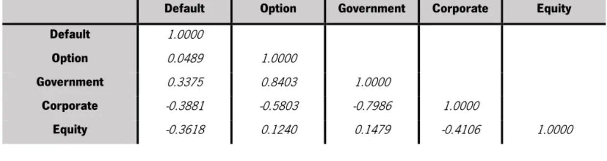
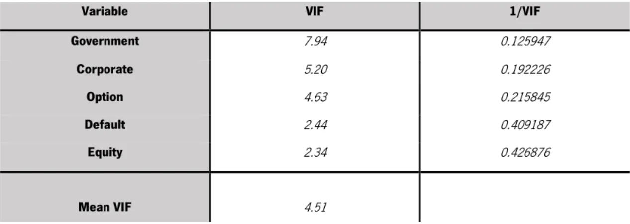
the sample includes funds that hold corporate and government debt. However, we ended up discarding the government factor (proxied by the excess returns of the BofA € 10+ years France Government Index) given some correlation issues that arose. In fact, as table 1 shows, the Government factor demonstrates a high correlation with the Option and the Corporate. To analyze whether this might raise multicollinearity problems, we further computed the variance inflation factors (VIF) for the five factors (including the government factor) and four factors (without the government factor). Checking on tables 3 and 4, we can observe that with the Government factor, abnormally high VIFs of the Government and Corporate factors appear (a value of 4 requires further investigation; 10 reveals severe multicollinearity). When excluding the Government factor (see Table 4), the VIF for all factors decrease to the normal state. Considering this analysis, we decided that the model should stick to the original four factors, without the Government factor. Table 2 presents the correlation matrix of the four factors and Table 5 presents the summary statistics of the four factors.

Table 1 – Correlation Matrix of coefficients of regression of 5-factor model

This table reports the correlation coefficients between the factors, where each cell indicates the correlation between two factors.

Default Option Government Corporate Equity

Default 1.0000

Option 0.0489 1.0000

Government 0.3375 0.8403 1.0000

Corporate -0.3881 -0.5803 -0.7986 1.0000

Equity -0.3618 0.1240 0.1479 -0.4106 1.0000

Table 2 – Correlation Matrix of coefficients of regression of 4-factor model

This table reports the correlation coefficients between factors, where each cell indicates the correlation between two factors.

Default Option Corporate MSCIFR

Default 1.0000

Option -0.4599 1.0000

Corporate -0.2093 0.2786 1.0000

Table 3 – Variance Inflation Factors for five factors

This table reports the Variance Inflation factors for factors for detecting the multicollinearity in five risk factors: Government, Corporate, Option and Default and Equity. All the variables are collected from December 2007 to December 2017.

Variable VIF 1/VIF

Government 7.94 0.125947 Corporate 5.20 0.192226 Option 4.63 0.215845 Default 2.44 0.409187 Equity 2.34 0.426876 Mean VIF 4.51

Table 4 – Variance Inflation Factors without Government factor

This table reports the Variance Inflation factors for factors for detecting the multicollinearity in four risk factors: Corporate, Option and Default and Equity. All the variables are collected from December 2007 to December 2017.

Variable VIF 1/VIF

Equity 2.29 0.436423

Default 2.17 0.461788

Corporate 1.88 0.530707

Option 1.36 0.734567

Mean VIF 1.93

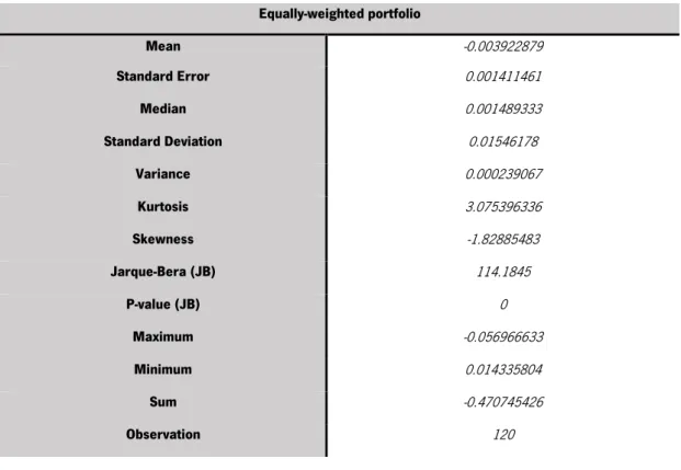
Besides analyzing individual fund performance, we also assess aggregate performance by constructing an equally-weighted portfolio of the funds. The summary statistics of the equally-weighted portfolio are presented in table 6.

Table 5 – Summary statistics of four factors

The table presents the summary statistics of four risk factors in which Corporate, Option and Default are primarily proxied by iBoxx € and BofA Merrill Lynch € Index family, and Equity is proxied by MSCI (Morningstar) French index. Each segment of factors consists of 120 observations. Jarque-Bera is a normality test that can determine whether the residuals of underlying variables in date set is likely to be normally distributed or not. The null hypothesis, variable being normally distributed, is rejected if P-value (JB) is lower than expected p-value (0.05 in this case).

Default Option Corporate Equity

Mean 0.007666131 -5.1E-05 -0.00283 -0.00211 Std. error 0.005832904 0.000902 0.001768 0.005064 Median 0.008908261 -0.00038 0.002417 0.005774 Std. Dev 0.063896267 0.009884 0.019372 0.055476 Variance 0.004082733 9.77E-05 0.000375 0.003078 Kurtosis 7.54211252 0.379281 5.306091 1.226182 Skewness -0.120045163 0.085786 -1.975 -0.84945 Jarque-Bera (JB) 284.70552 0.86645 218.7855 21.949 P-value (JB) 0 0.64841 0 0 Maximum -0.301279623 -0.0256 -0.09421 -0.18887 Minimum 0.288423717 0.028709 0.030476 0.125359 Sum 0.919935695 -0.00615 -0.33962 -0.25299 Observations 120 120 120 120

Table 6 – Summary statistics of equally-weighted portfolio

The table reports the summary statistics of monthly excess return of the equally-weighted portfolio documented from January, 2008 to December, 2017, containing 120 observations. Jarque-Bera is a normality test that can determine whether the residuals of underlying variables in date set is likely to be normally distributed or not. The null hypothesis, variable being normally distributed, is rejected if P-value (JB) is lower than expected p-value (0.05 in this case).

5. EMPIRICAL RESULTS

This chapter is divided into two parts. The first part presents the results regarding the performance of individual funds and the equally-weighted portfolio from January 2008 to December 2017. Then, we present the contingency tables results to assess fund performance persistence

5.1. Performance evaluation using the four-factor model

We start by evaluating performance both at the individual fund level and at the aggregate level, by evaluating the performance of the equally-weighted portfolio of funds. Fund performance is evaluated with the four-factor model presented in equation (2). Due to the fact that this type of time-series data it is likely affected by autocorrelation and heteroskedasticity, we use Newey-West (1987) estimators (Newey–West standard errors for coefficients estimated by OLS regression) to correct the errors.

We further use the Wald test, which tests the null hypothesis that all the coefficients of the four factors (Default, Option, Corporate, and Equity) are simultaneously equal to 0.

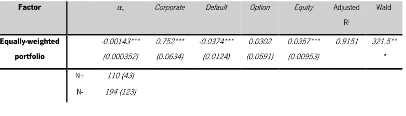
Table 7 presents the regression results of the four-factor model.

Equally-weighted portfolio Mean -0.003922879 Standard Error 0.001411461 Median 0.001489333 Standard Deviation 0.01546178 Variance 0.000239067 Kurtosis 3.075396336 Skewness -1.82885483 Jarque-Bera (JB) 114.1845 P-value (JB) 0 Maximum -0.056966633 Minimum 0.014335804 Sum -0.470745426 Observation 120

Table 7 – Performance evaluation using the four-factor model

This table presents estimates of performance for an equally-weighted portfolio of French bond funds using the four-factor model of equation (2). Corporate corresponds to the monthly excess returns of iBoxx € Corporate Index. Excess returns were computed using the one-month Euribor as the risk-free rate. Default is computed as the difference in returns between the BofA € Global High Yield TR Index and the iBoxx € France Sovereign TR Index. Option corresponds to the difference in return between the BofA € Asset-Backed & Mortgage-Backed Security (ABS&MBS) TR Index and the iBoxx € France Sovereign TR Index. Equity corresponds to the monthly excess returns of the MSCI France Index. Adjusted R2 is the adjusted coefficient of determination. Wald indicates the result of the Wald test for the null hypothesis that the

coefficients of the corporate, default, option, and equity factors are jointly equal to zero. The number of funds portfolio with positive (N+) and negative (N-) estimates are presented. The number of funds whose estimates are statistically significant at least at the 5% level are presented in parentheses. The asterisks are used to represent the statistically significant coefficients at the 1% (***), 5% (**) and 10% (*) significance levels, based on heteroskedasticity and autocorrelation adjusted errors (following Newey and West, 1987).

Factor αp Corporate Default Option Equity Adjusted

R2 Wald Equally-weighted portfolio -0.00143*** (0.000352) 0.752*** (0.0634) -0.0374*** (0.0124) 0.0302 (0.0591) 0.0357*** (0.00953) 0.9151 321.5** * N+ 110 (43) N- 194 (123)

With regards to fund performance at the aggregate level, the alpha of the equally weighted portfolio of funds is negative and statistically significant at the 1% level, indicating a that French bond funds underperform the benchmark. Relative to the risk factors, the coefficients of the Corporate and Equity factors are positive and statistically significant at 1% level; the coefficient of Default factor is negative and statistically significant at the 1% level: and the coefficient of the Option factor is positive but not statistically significant.

In terms of the performance of individual funds, poorly performing funds dominate. Among the 304 funds, 110 funds delivery positive alphas but only 43 out of them are statistically significant at the 5% level. In turn, 194 funds produce negative alphas, of which 123 are statistically significant at the 5% level. Funds with statistically significant positive alphas represent 14.1% of the sample compared to 40.5% of the funds with statistically significant negative alphas.

In relation to the performance of the model, as can be in Table 7, the Adjusted R-square reaches 0.9151, indicating a very good explanatory power of the model. The results of the Wald allow us to reject the null hypothesis that the coefficients of Corporate, Default, Option and Equity are jointly equal to zero. 5.2 Performance persistence

calculated through 36-month rolling regression windows. We then calculate the cumulative alphas, for alternative time periods: months, 12-months and 24-months. The contingency tables based on 6-months periods comprises 14 periods and 304 funds; the 12-month contingency table comprises 7 periods and 295 funds and the 24-month contingency table covers 3 periods and 272 funds.

In the assessment of performance persistence using contingency tables, we used three statistical tests: Malkiel’s (1995) Z-statistic, Brown and Goetzman’s (1995) Odds ratio and Z-statistic and Kahn and Rudd’s (1995) Chi-square. Under each test, the null hypothesis that past performance is unrelated to future performance. Under Malkiel’s (1995) repeat winner strategy, if repeat winner or repeat loser frequencies surpass 0.5, and its Z-test is above 0, we reject the null hypothesis and claim that there is performance persistence. For Brown and Goetzman’s (1995) Odds ratio, the performance persistence will be indicated when the Odds ratio and Z-statistic surpass 1, and p-value is lower than 0.05. Under Kahn and Rudd’s (1995) Chi-square, the null hypothesis is rejected when Chi-square is bigger than the critical value, 3.8414 (0.05).

The following tables report the results for the 6-month, 12-month and 24-month contingency tables, respectively.

From Table 8, we observe performance persistence from 8 out of 14 periods (periods 2, 4, 5, 6, 7, 11, 12, 14) according to Malkiel’s (1995) test. Moving to the Odds ratio and Z-statistic of Brown and Goetzman (1995), 9 out of 14 periods (periods 2, 4, 5, 6, 7, 11, 12, 13, 14) show evidence of performance persistence. Kahn and Rudd’s (1995) Chi-square test indicates 10 out of 14 periods for which we can reject the null hypothesis. At the overall level, the results also indicate persistence of performance of winners and losers.

Table 8 – Contingency tables for 6-month periods

The table reports the test results from repeat winner strategy and Z-test (Malkiel, 1995), Odds ratio and Z-statistic (Brown and Goetzman, 1995) and Chi-square (Kahn and Rudd, 1995) based on 6-month contingency table. WL, LW, WL, and LL refer to repeat winner, loser-loser, winner-loser and repeat loser, identified by comparing the cumulative alphas of each fund with the median value from each period. Regarding Malkiel’s (1995) test, REPEAT W and REPEAT L indicates the percentage of repeat winners and losers, and Z-TEST W and L their corresponding Z- test. Regarding Brown and Goetzmann’s (1995) test, Z-STAT stands for the Z-statistic of the Odds ratio, and LOG indicates standard error as mentioned in chapter 3. Regarding Kahn and Rudd’s (1995) test, CHI-SQ represents the Chi-square statistics. Figures in italic and bold indicate statistical significance at the 5% level.

Period WW LW WL LL

Malkiel Brown and Goetzmann Kahn and Rudd

REPEA T W

Z-TEST

W REPEAT L Z-TEST L p-value ODDS RATIO STAT Z- (LOG) p-value CHI-SQ value p-

2 76 34 35 77 0.685 3.891 0.6937 4.081 0.000 4.918 5.492 0.290 0.000 31.802 0.000 3 48 63 68 49 0.4138 -1.857 0.4375 -1.3229 0.063 0.5490 -2.237 0.2680 0.025 5.298 0.021 4 82 39 37 84 0.689 4.125 0.683 4.057 0.000 4.773 5.641 0.277 0.000 33.537 0.000 5 88 34 33 90 0.727 5.000 0.726 5.029 0.000 7.059 6.817 0.287 0.000 50.331 0.000 6 92 38 30 101 0.754 5.613 0.727 5.344 0.000 8.151 7.399 0.284 0.000 60.977 0.000 7 86 49 45 91 0.656 3.582 0.650 3.550 0.000 3.549 4.960 0.255 0.000 25.723 0.000 8 76 63 60 76 0.5588 1.372 0.5468 1.1026 0.170 1.528 1.748 0.243 0.081 3.124 0.0772 9 74 67 64 77 0.5362 0.851 0.5347 0.8333 0.395 1.329 1.190 0.239 0.234 1.546 0.2137 10 80 65 71 76 0.5298 0.732 0.5390 0.9264 0.464 1.317 1.174 0.235 0.240 1.726 0.1889 11 90 57 55 90 0.620 2.907 0.612 2.722 0.000 2.584 3.943 0.241 0.000 15.863 0.000 12 103 49 43 107 0.705 4.965 0.686 4.644 0.000 5.231 6.607 0.250 0.000 46.450 0.000 13 85 66 67 85 0.5592 1.460 0.5629 1.5462 0.144 1.634 2.121 0.232 0.034 4.525 0.033 14 94 57 57 94 0.623 3.011 0.623 3.011 0.000 2.719 4.214 0.237 0.000 18.133 0.000 TOTAL 1074 681 665 1097 0.618 9.808 0.617 9.866 0.000 2.602 13.72 0.069 0.000 193.971 0.000

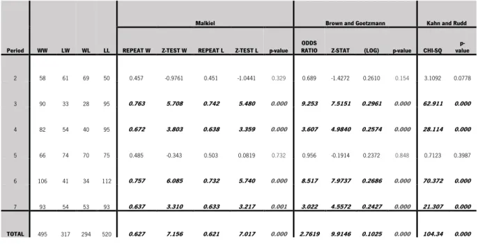
Table 9 presents the results of the contingency table of 12-month periods. As we can observe, 4 out 7 periods (periods 3,4,6,7) show evidence of the persistence according to all the tests performed: Malkiel’s (1995) repeat winner/loser test, Brown and Goetzmann (1995) Odds ratio and Z-statistic and the Chi-Square test. Considering the overall period, the results also indicate performance persistence.

Table 9 – Contingency tables for 12-month periods

The table reports the test results from repeat winner strategy and Z-test (Malkiel, 1995), Odds ratio and Z-statistic (Brown and Goetzman, 1995) and Chi-square (Kahn and Rudd, 1995) based on 6-month contingency table. WL, LW, WL, and LL refer to repeat winner, loser-loser, winner-loser and repeat loser, identified by comparing the cumulative alphas of each fund with the median value from each period. Regarding Malkiel’s (1995) test, REPEAT W and REPEAT L indicates the percentage of repeat winners and losers, and Z-TEST W and L their corresponding Z- test. Regarding Brown and Goetzmann’s (1995) test, Z-STAT stands for the Z-statistic of the Odds ratio, and LOG indicates standard error as mentioned in chapter 3. Regarding Kahn and Rudd’s (1995) test, CHI-SQ represents the Chi-square statistics. Figures in italic and bold indicate statistical significance at the 5% level.

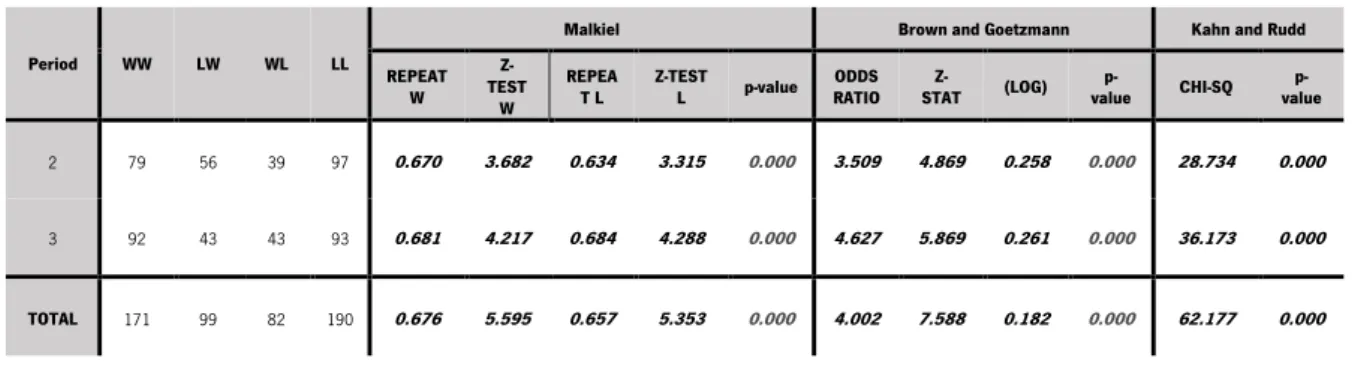
Table 10 presents the contingency table results using 24-month periods. The results show evidence of performance persistence both of winners and losers under all the tests.

Period WW LW WL LL

Malkiel Brown and Goetzmann Kahn and Rudd

REPEAT W Z-TEST W REPEAT L Z-TEST L p-value RATIO ODDS Z-STAT (LOG) p-value CHI-SQ value p-

2 58 61 69 50 0.457 -0.9761 0.451 -1.0441 0.329 0.689 -1.4272 0.2610 0.154 3.1092 0.0778 3 90 33 28 95 0.763 5.708 0.742 5.480 0.000 9.253 7.5151 0.2961 0.000 62.911 0.000 4 82 54 40 95 0.672 3.803 0.638 3.359 0.000 3.607 4.9840 0.2574 0.000 28.114 0.000 5 66 74 70 75 0.485 -0.343 0.503 0.0819 0.732 0.956 -0.1914 0.2372 0.848 0.7123 0.3987 6 106 41 34 112 0.757 6.085 0.732 5.740 0.000 8.517 7.9737 0.2686 0.000 70.372 0.000 7 93 54 53 93 0.637 3.310 0.633 3.217 0.001 3.022 4.5572 0.2427 0.000 21.307 0.000 TOTAL 495 317 294 520 0.627 7.156 0.621 7.017 0.000 2.7619 9.9146 0.1025 0.000 104.34 0.000

Table 10 – Contingency tables for 24-month periods

The table reports the test results from repeat winner strategy and Z-test (Malkiel, 1995), Odds ratio and Z-statistic (Brown and Goetzman, 1995) and Chi-square (Kahn and Rudd, 1995) based on 6-month contingency table. WL, LW, WL, and LL refer to repeat winner, loser-loser, winner-loser and repeat loser, identified by comparing the cumulative alphas of each fund with the median value from each period. Regarding Malkiel’s (1995) test, REPEAT W and REPEAT L indicates the percentage of repeat winners and losers, and Z-TEST W and L their corresponding Z- test. Regarding Brown and Goetzmann’s (1995) test, Z-STAT stands for the Z-statistic of the Odds ratio, and LOG indicates standard error as mentioned in chapter 3. Regarding Kahn and Rudd’s (1995) test, CHI-SQ represents the Chi-square statistics. Figures in italic and bold indicate statistical significance at the 5% level.

Period WW LW WL LL

Malkiel Brown and Goetzmann Kahn and Rudd

REPEAT W Z-TEST W REPEA

T L Z-TEST L p-value RATIO ODDS STAT Z- (LOG) value p- CHI-SQ value

p-2 79 56 39 97 0.670 3.682 0.634 3.315 0.000 3.509 4.869 0.258 0.000 28.734 0.000

3 92 43 43 93 0.681 4.217 0.684 4.288 0.000 4.627 5.869 0.261 0.000 36.173 0.000

TOTAL 171 99 82 190 0.676 5.595 0.657 5.353 0.000 4.002 7.588 0.182 0.000 62.177 0.000

After analyzing three contingency tables, we conclude that there is evidence of performance persistence of winners and losers at the 6-month, 12-month and 24-month periods.

6. CONCLUSIONS

In the past several decades a set of studies have analyzed the performance of mutual funds. Despite the growth and relevance of bond funds, most studies focus on equity funds and the performance of bond funds is less explored. After the seminal paper of Blake et al. (1993), the research on bond funds gradually developed. Despite this, extant papers on bond funds primarily address bond fund performance rather than their performance persistence. In addition, previous studies favor the US market and Continental Europe instead of dealing with more specific areas.

In this paper, we assess performance persistence in the French bond mutual fund market. In particular, this dissertation examines the consistency in performance of 304 bond funds from February 2008 to December 2017. We first evaluated overall fund performance at the individual fund level and aggregate level (through the equally-weighted portfolio) based on a four-factor model that includes the bond, default, option and equity factors. To assess performance persistence, we initially conduct rolling window regressions to obtain the monthly alphas (as in Ferreira et al., 2013) Afterwards, we computed the cumulative monthly alphas for periods of 6-months, 12-months and 24-months and constructed two-way contingency tables for those periods. We used the Repeat Winner test (as in Malkiel, 1995), the Odds Ratio Z-statistic (as in Brown and Goetzmann, 1995) and the Chi-Square test (as in Khan and Rudd,

1995) to evaluate the statistical significance of performance persistence.

In terms of overall performance, the results indicate that it is apparent that few funds delivered superior performance from January 2008 to December 2017. The equally-weighted portfolio performed poorly compared to the benchmark. In terms of individual funds with statistically significant underperformance account for 40.5% of the total. Accordingly, we could claim that French bond fund did not produce overall positive performance from 2008 to 2017. We further analyzed performance persistence to check whether the best/worst funds perform consistently in subsequent periods. The results show that that performance persistence strongly holds for 6-month, 12-month and 24-month periods and both for winners and losers. Hence, we could summarize that there are “hot hands” as well as “cold hands” in French bond mutual funds from 2008 to 2017.

Several limitations to this study need to be acknowledged. First, regarding the dataset, it is not free of survivorship-bias, as only active funds are considered. For future research, the use of survivorship bias-free databases would be recommended. Secondly, the coverage of the variety of bond funds is not exhaustive: for instance, convertible bonds, global bonds, inflation-linked bonds, etc. are not included in the dataset. Thirdly, as we stated before, our conclusion relies on the use of unconditional models in evaluating performance. This choice was motivated by practical constraints in the computation of monthly alphas and probably will not lead to relevant biases since the rolling window procedure used to calculate monthly alphas somewhat accounts for time-varying risk and performance. Anyhow, we suggest that the conditional model could be used in assessing overall performance (previous to the persistence analysis). Lastly, this study has not considered management fees, as in Polwtioon and Tawatnuntachai (2006), Clare et al. (2019) and Huji and Derwall (2008).. Therefore, we suggest that future studies on this topic take this issue into account. Notwithstanding these limitations, we believe this study sheds light on the persistence of France-based bond funds, which had not been explored yet.

REFERENCES

Association Française de la Gestion fnancière. (2017). France, a major player in Asset Management among Europe. Retrieved from https://www.afg.asso.fr/en/key-data-3/

Association Française de la Gestion fnancière. (2018). France Stat. Data – November 2018. Retrieved from https://www.afg.asso.fr/en/france-stat-data-september2018-2/

Association Française de la Gestion fnancière. (2016). Competitiveness of the Paris Financial Center. Paris: AFG Communication Department

Autorité des marchés financiers. (2015). Study of liquidity in French bond markets. Paris: Autorité des marchés financiers.

Blake, C. R., Elton, E. J., & M. J, Gruber, M. J. (1993). The performance of bond mutual funds. The Journal of Business, 66, 371-403.

Brown, S., & Goetzmann, W. (1995). Performance persistence. Journal of Finance, 50, 679–698. Carpenter, J. N., & Lynch, A. W. (1999). Survivorship bias and attrition effects in

measures of performance persistence. Journal of Financial Economics, 54(3), 337- 374.

Carhart, M. (1997), On persistence in mutual fund performance. Journal of Finance, 52, 57–82. Chen, Z., & P. J. Knez, (1996). Portfolio performance measurement: Theory and applications. The Review of Financial Studies (Summer), 9, 511-555.

Christopherson, J. A, Ferson, W. E., & Glassman, D. A. (1998). Conditioning manager alphas on economic information: Another look at the persistence of performance. Review of Financial Studies, 11, 111–142.

Christensen, R. (1990). Log-linear models. New York: Springer-Verlag.

Clare, A., O'Sullivan, N., Sherman, M. and Zhu, S. (2019). The performance of US bond mutual funds. International Review of Financial Analysis, 61, 1-8

Derwall, J., & Koedijk, K. (2009). Socially responsible fixed‐income funds. Journal of Business Finance & Accounting, 36(1‐2), 210-229.

Detzler, M. L. (1999). The performance of global bond mutual funds. Journal of Banking and Finance, 23, 1195-1217.

Droms, G., & Walker, A. (2006). Performance persistence of fixed-income mutual funds. The Journal of Economics and Finance, 30, 337-355

Elton, E. J., Gruber, M. J., & Blake, C. R. (1995). Fundamental Economic Variables, expected returns, and bond fund performance. The Journal of Finance, 50(4), 1229-1256.

Elton, E. J., Gruber, M. J., & Blake, C. R. (1996b). Survivorship bias and mutual fund performance. Review of Financial Studies, 9, 1097–1120.

Elton, E. J., Gruber, M. J., Das, S., & Blake, C. R. (1996a). The persistence of risk-adjusted mutual fund performance. Journal of Business, 69, 133–157.

European Fund and Asset Management Association. (2018). Asset Management in Europe: An overview of the Asset Management Industry 10th Edition Facts and figures. Brussels: European Fund and Asset

Management Association.

Ferreira, M., Keswani, A., Miguel, A. and Ramos, S. (2012). The Determinants of Mutual Fund Performance: A Cross-Country Study. Review of Finance, 17(2), 483-525.

Gallo, J. G., Lockwood, L. J., & Swanson, P. E. (1997). The performance of international bond funds. International Review of Economic& Finance, 6(1), 17-35

Grinblatt, M., & Titman, S. (1992). The persistence of mutual fund performance. Journal of Finance, 47(5), 1977-1984.

Gudikunst, A., & Mccarthy, J. (1992). Determinants of bond mutual fund performance. The Journal of Fixed Income (Summer), 2(1), 95-101

Hendricks, D., Patel, J., & Zeckhauser, R. (1993). Hot hands in mutual funds: Short run persistence of relative performance, 1974–1988. Journal of Finance, 48, 93–130.

Huij, J., & Derwall, J. (2008). ‘Hot hands’ in bond funds. Journal of Banking & finance, 32(4), 559-572. Jensen, M. (1968). The performance of mutual funds in the period 1945–1964. Journal of Finance, 48, 389–416.

Kahn, R. N., & Rudd, A. (1995). Does historical performance predict future performance? Financial Analysts Journal, 51, 43-52.

Leite, P., & Cortez, M. (2018). The performance of european SRI funds investing in bonds and their comparison to conventional funds. Investment Analysts Journal, 47, 65-79

Malkiel, B.G. (1995). Returns from investing in equity mutual funds 1971 to 1991. Journal of Finance ,50, 549–572

Newey, W. K., & West, K. D. (1987). Hypothesis testing with efficient method of moments estimation. International Economic Review, 28(3), 777-787.

Otten, R., & Bams, D. (2002). European mutual fund performance. European Financial Management, 8, 75-101.

Polwitoon, S., & Tawatnuntachai, O. (2006). Diversification benefits and persistence of US-based global bond funds. Journal of Banking & Finance, 30(10), 2767-2786.

Silva, F. C., Cortez, M. C., & Armada, M. J. R. (2003). Conditioning information and European bond fund performance. European Financial Management, 9, 201-230

Silva, F. C., Cortez, M. C., & Armada, M. J. R. (2005). The persistence of European bond fund performance: Does conditioning information matter? International Journal of Business, 10(4), 342-362. Silva, F., Cortez, M. C., & Armada, M. R. (2005). The persistence of European bond

fund performance: Does conditioning information matter? International Journal of

Business, 10(4), 341-361.

APPENDIX

NAME CODE ASSET TYPE BASE OR ST DATE LIPPER GLB CLASFN.

ABN AMRO EURO SUSTAINABLE BONDS C 13293X(RI) Bond 1998/6/25 Bond EUR

AG2R LA MONDIALE AGGREGATE EURO 89299J(RI) Bond 2002/4/23 Bond EUR

ALCIS ALPHA OBLIGATIONS CREDIT IALCIS GESTION 88349E(RI) Bond 2013/4/17 Bond EUR

ALCIS ALPHA OBLIGATIONS CREDIT P 41134K(RI) Bond 2006/8/16 Bond EUR

ALCIS CAPI ALCIS GESTION 30233U(RI) Bond 2005/1/24 Bond EUR

ALLIANZ EURO HIGH YIELD I GLOBAL INVRS.FRN. 413198(RI) Bond 2006/10/26 Bond EUR High Yield

ALLIANZ EURO HIGH YIELD I TD 89559M(RI) Bond 2013/7/17 Bond EUR High Yield

ALLIANZ EURO OBLIG COURT TERME ISR R C 70134J(RI) Bond 2014/8/6 Bond EUR Short Term

ALLZ.ER.OBLIG CRT.TERME ISR GLB.INVRS.FRN. 9061Q3(RI) Bond 2010/9/10 Bond EUR Short Term

ALM OBLIG EURO ISR IC 14363J(RI) Bond 2001/7/10 Bond EUR

ALM SOUVERAINS EURO ISR 7076NQ(RI) Bond 2003/3/26 Bond EMU Government

ALPHA COURT TERME PALATINE ASTMGMT. 14732N(RI) Bond 2001/10/25 Bond EMU Government ST

AMUNDI CREDIT 1-3 EURO - P (C) 256318(RI) Bond 2009/3/12 Bond EUR Corporates Short Term

AMUNDI CREDIT EURO - I (C) 29465K(RI) Bond 1996/1/2 Bond EUR Corporates

AMUNDI CREDIT EURO ISR - I (C) 67077U(RI) Bond 2004/1/22 Bond EUR Corporates

AMUNDI EURO BOND ESR - N (C) 2562JG(RI) Bond 2006/5/2 Bond EMU Government

AMUNDI FRN.LCL OBLIG REVENU TRIM 4 31941U(RI) Bond 2005/9/26 Bond EUR

AMUNDI FRN.LCL OBLIG REVENU TRIM 5 880501(RI) Bond 2005/9/26 Bond EUR

AMUNDI OBLIG 1-3 EURO I (C) 67865E(RI) Bond 1996/1/2 Bond EUR Short Term

AMUNDI OBLIG 1-3 EURO P (C) 77807U(RI) Bond 2009/8/7 Bond EUR Short Term

AMUNDI OBLIG 5-7 EURO - I (D) 7289H5(RI) Bond 2011/10/6 Bond EUR Long Term

AMUNDI OBLIG 5-7 EURO - I2 (C) 9387QX(RI) Bond 1996/1/31 Bond EUR Long Term

AMUNDI OBLIG EURO - D 15345P(RI) Bond 1996/8/23 Bond EUR

ANTARIUS OBLI 1-3 ANS (C) 9331TC(RI) Bond 2002/3/21 Bond EUR Short Term

AVIVA INVESTORS EURO AGGREGATE I 13381K(RI) Bond 2014/11/12 Bond EUR

AVIVA INVESTORS EURO CR. BONDS 1 TO 3 FRANCE 68156U(RI) Bond 1996/1/2 Bond EUR Short Term

AVIVA INVESTORS OBGS. VARIABLES A FRANCE 35714F(RI) Bond 2009/10/16 Bond EUR Short Term

AVIVA INVRS.CR.EUROPE (C) GEST.D'ACTIFS 880142(RI) Bond 2003/7/3 Bond EUR Corporates

AVIVA INVRS.OBGS. VARIABLES GEST.D'ACTIFS 880141(RI) Bond 2006/4/13 Bond EUR Short Term

AVIVA OBLIREA AVIVA GESTION D ACTIFS 14908K(RI) Bond 1996/7/26 Bond EMU Government

AVIVA RENDEMENT EUROPE 14076R(RI) Bond 1996/7/26 Bond EUR

AVIVA SIGNATURES EUROPE AVIVA GESTION D

ACTIFS 13310L(RI) Bond 2001/12/28 Bond EUR Corporates

AXA EURO 7 10 D 880109(RI) Bond 1996/1/2 Bond EUR Long Term

AXA EURO AGGEREGATE SHORT DURATION D EUR 880083(RI) Bond 1999/7/7 Bond EUR Medium Term

AXA EURO CREDIT (D) AXA INVESTMENT PARIS 880052(RI) Bond 1999/6/25 Bond EUR Corporates

AXA EURO OBLIGATIONS D EUR 880378(RI) Bond 1996/7/26 Bond EUR

AXA PREMIERE CATEGORIE D INV.MANAGERS PARIS 50586K(RI) Bond 1996/7/26 Bond EMU Government

AXA PREMIRE CATGORIE C EUR 880150(RI) Bond 1996/7/30 Bond EMU Government

BATI CREDIT PLUS SMA GESTION 67849P(RI) Bond 2007/5/18 Bond EUR Corporates

BATI PREMIERE (C) INVESTIMO 8696Q4(RI) Bond 1996/7/26 Bond EMU Government

BATI TRESORERIE SMA GESTION 51520P(RI) Bond 2009/8/4 Bond EUR

BFT CREDIT OPPORTUNITES PLUS - P (C) 9366LH(RI) Bond 2013/12/13 Bond EUR High Yield

BFT LCR (C) 29574U(RI) Bond 2008/1/4 Bond EMU Government ST

BFT LCR NIVEAU 2 C 87732U(RI) Bond 2015/2/18 Bond EUR

BNP PARIBAS BOND CASH EQUIVALENT - CLASSIC

(C) 29599E(RI) Bond 2004/9/23 Bond EUR Short Term

BNP PARIBAS BOND CASH EQUIVALENT MANDAT 30117V(RI) Bond 2012/10/10 Bond EUR Short Term

BNP PARIBAS OBLI CT CLASSIC D 9061FU(RI) Bond 2004/9/28 Bond EUR Short Term

BNP PARIBAS OBLI CT I 299584(RI) Bond 2005/1/11 Bond EUR Short Term

BNP PARIBAS OBLI ENTREPRISES CLASSIC 13325J(RI) Bond 1997/6/5 Bond EUR Corporates

BNP PARIBAS OBLI FLEXIBLE CLASSIC D 28143W(RI) Bond 2004/9/21 Bond EUR

BNP PARIBAS OBLI LONG TERME CLASSIC D 93072W(RI) Bond 2004/9/28 Bond EUR Long Term

BNP PARIBAS OBLI RESPONSABLE CLASSIC D 13207U(RI) Bond 2003/11/24 Bond EMU Government

BNP PARIBAS OBLI RESPONSABLE M 53756W(RI) Bond 2011/6/15 Bond EMU Government

BSO COURT TERME C 2620PY(RI) Bond 1996/1/5 Bond EUR Short Term

CAM GESTION EUROBLIG R 26104R(RI) Bond 2008/8/4 Bond EUR

CAM GESTION OBLICYCLE CREDIT R 54647C(RI) Bond 2008/12/16 Bond EUR Corporates

CAMGESTION CAPI OBLIG CARDIF GESTION D

ACTIFS 25737T(RI) Bond 2002/8/12 Bond EMU Government LT

CAMGESTION OBLICYCLE CREDIT CLASSIC 258351(RI) Bond 2009/1/16 Bond EUR Corporates

CAPITOP REVENUS (D) 87270F(RI) Bond 2002/6/26 Bond EUR

CARMIGNAC GESTION SECURITE FCP CAP. 77296M(RI) Bond 1996/1/1 Bond EUR Short Term

CARMIGNAC SECURITE A EUR YDIS 15436M(RI) Bond 2012/6/21 Bond EUR Short Term

CAVA CT I GESTION 880445(RI) Bond 2011/6/15 Bond EUR

CIC OBLI COURT TERME (C) CIC BANQUES 69886W(RI) Bond 2002/4/22 Bond EUR Short Term

CIC OBLIGATIONS C CIC ASSET MANAGEMENT 15470R(RI) Bond 1996/8/2 Bond EUR

CIPEC COMPARTIMENT OBLIGATIONS 8701CZ(RI) Bond 2010/8/2 Bond EUR

CLICHY PREMIERE (C) FORTIS INV.MAN.FRANCE 13011V(RI) Bond 2002/4/19 Bond EUR Corporates

CM-CIC ASSOCIATIONS COURT TERME D 13315M(RI) Bond 2000/2/22 Bond EUR Short Term

CM-CIC LCR OBLI COURT TERME C 87308R(RI) Bond 1996/1/5 Bond EUR Short Term

CM-CIC OBLI 7-10 C 880952(RI) Bond 1996/10/17 Bond EUR Long Term

CNP ASSUR CAPI R NATIXIS ASSET MAN. 13344M(RI) Bond 2012/7/3 Bond EUR Medium Term

CNP ASSUR CAPI(C) CAISSE NATIONALE 27369D(RI) Bond 1996/8/22 Bond EUR Medium Term

CNP ASSUR EURO 74094K(RI) Bond 1996/4/30 Bond EMU Government LT

CNP ASSUR IXIS CREDIT CDC IXIS ASSET MGMENT 13344Q(RI) Bond 2003/8/1 Bond EUR Corporates

CNP ASSUR OBLIG R E NATIXIS ASSET MAN. 32858V(RI) Bond 2010/12/29 Bond EMU Government

CNP ASSUR OBLIG(D) CDC IXIS 258880(RI) Bond 1996/4/30 Bond EMU Government

CNP ASSUR UBSCREDIT BNP PARIBAS SECURITIES

SVS.E 51277H(RI) Bond 2006/2/21 Bond EUR Corporates

CONFIANCE SOLIDAIRE D CREDIT COOPERATIF 9812T4(RI) Bond 2007/10/24 Bond EUR

CONFIANCE SOLIDAIRE FDA 256405(RI) Bond 2008/10/31 Bond EUR

COPERNIC OBLIGATION 77446P(RI) Bond 1989/7/24 Bond EUR

COVEA EURO SOUVERAIN (C) MMA FINANCE 13426L(RI) Bond 1998/5/27 Bond EMU Government

COVEA EURO SPREAD C 13300X(RI) Bond 2011/7/20 Bond EUR

COVEA EURO SPREAD D FINANCE 880429(RI) Bond 1999/2/8 Bond EUR

COVEA MOYEN TERME (C) 86575M(RI) Bond 1998/4/2 Bond EUR Short Term

COVEA OBLIGATIONS D COVEA FINANCE 13313K(RI) Bond 1996/8/22 Bond EUR

CPR 7-10 EURO SR - S 54376M(RI) Bond 2008/11/14 Bond EMU Government LT

CPR EURO GOV+ MT - P 75508V(RI) Bond 1996/1/4 Bond EMU Government MT

DNCA SERENITE PLUS C CM CIC SECURITIES 74995V(RI) Bond 2011/3/2 Bond EUR Short Term

DNCA SERENITE PLUS I 87131D(RI) Bond 2011/2/21 Bond EUR Short Term

DOM OPPORTUNITES 1-3 C 68661C(RI) Bond 2012/5/4 Bond EUR Short Term

ECHIQUIER CREDIT EUROPE A 9389CF(RI) Bond 2007/7/20 Bond EUR Corporates

ECHIQUIER CRT.TERME FINC.DE L'ECHIQUIER 87901T(RI) Bond 2010/1/14 Bond EUR Short Term

ECOFI CONTRAT COOPERATIF 2 ECOFI

INVESTISSEMENTS 92761R(RI) Bond 2012/11/28 Bond EUR

ECOFI CONTRAT SOLIDAIRE B 75570J(RI) Bond 2011/7/26 Bond EUR Corporates

ECOFI HIY.INMS.GROUPE CREDIT COOPERATIF 68055H(RI) Bond 2011/3/9 Bond EUR High Yield

ECOFI OPTIM 12 MOIS 289861(RI) Bond 2009/9/24 Bond EUR Short Term

ECOFI QUANT OBLIGATIONS ECOFI

INVESTISSEMENTS 77326Q(RI) Bond 1996/1/4 Bond EMU Government LT

ECOFI TAUX VARIABLE I INVESTISSEMENTS 30978R(RI) Bond 2011/6/27 Bond EUR Short Term

ECUREUIL OBLI MOYEN TERM (C) ECUREUIL

GESTION FCP 88796K(RI) Bond 2005/5/10 Bond EUR

EGAMO OBLIGATION COURT TERME 29342R(RI) Bond 2013/5/24 Bond EUR Short Term

EPARCOURT D 77136H(RI) Bond 2004/8/9 Bond EMU Government ST

EPARGNE ETHIQUE OBGS.C ECOFI

EPARGNE OBLIG EURO C 13387C(RI) Bond 2003/2/3 Bond EMU Government MT

EPARGNE SOLIDAIRE(D) EFIGESTION (CCCC) 260966(RI) Bond 1996/1/4 Bond EUR

EQUI-TRESORERIE PLUS 32990F(RI) Bond 1999/9/15 Bond EUR Short Term

ETOILE OBLI TAUX PLUS C 13355C(RI) Bond 2006/3/20 Bond EUR Medium Term

EURO BONDS VISION(C) GIFAO INVESTISSEMENT 13444D(RI) Bond 1996/1/4 Bond EUR Corporates

FAIM ET DEVELOPPEMENT HORIZON ECOFI INMS. 74084Q(RI) Bond 2001/1/18 Bond EUR

FAUVETTES MEESCHAERT ASSET MANAGEMENT 256601(RI) Bond 2010/12/24 Bond EUR

FEDERAL OBLIGATION PREMIERE LCR 69213T(RI) Bond 1996/1/2 Bond EUR Short Term

FEDERAL OBLIGATION VARIABLE ISR I 9466FQ(RI) Bond 2010/4/16 Bond EUR Corporates Short Term

FINCH C 14930D(RI) Bond 2012/8/24 Bond EUR Medium Term

FONDOBLIG (C) LCF ROTHSCHILD AM 13351X(RI) Bond 2001/12/21 Bond EUR

FORCE OPTIMA LCR 13360F(RI) Bond 1998/5/15 Bond EMU Government

FRANCE TRESOR CAPITAL D 30453H(RI) Bond 1996/10/22 Bond EUR

FRUCTI OBLI EURO COURT TERME D NATIXIS

ASTMGMT. 77543D(RI) Bond 2005/3/3 Bond EMU Government ST

FUNDY 8859VJ(RI) Bond 2011/8/12 Bond EUR

FUNDY 0 R C 8943P9(RI) Bond 2014/1/6 Bond EUR

GALAXIE G 54413R(RI) Bond 2008/11/6 Bond EUR

GALAXIE OBLIGATAIRE 2 C 880969(RI) Bond 2008/11/21 Bond EUR

GAN RENDEMENT(D) GAN - GROUPAMA 26589U(RI) Bond 1996/8/23 Bond EMU Government

GERER REGULARITE PLUS GERER CONSEIL 13371H(RI) Bond 2002/11/21 Bond EMU Government ST

GESTION PRIVEE RENDEMENT P (C) 8741W8(RI) Bond 1996/1/5 Bond EUR Long Term

GOUVERNANCE ETHIQUE COURT TERME A 259860(RI) Bond 2009/4/8 Bond EUR Short Term

GPK VARIFONDS (C) GPF GESTION 256635(RI) Bond 1996/1/5 Bond EUR Medium Term

GROUPAMA CR.ER.I CAP.EUR 67077Q(RI) Bond 1997/10/8 Bond EUR Corporates

GROUPAMA CR.ER.M ASST. MANAGEMENT 67613W(RI) Bond 2009/6/11 Bond EUR Corporates

GROUPAMA CR.ER.N CAP.EUR 35759M(RI) Bond 2006/4/26 Bond EUR Corporates

GROUPAMA CREDIT EURO ISR I C 256637(RI) Bond 2009/3/12 Bond EUR Corporates