Management Science Letters 5 (2015) 577–590 Contents lists available at GrowingScience
Management Science Letters
homepage: www.GrowingScience.com/msl
Conditional selectivity performance of Indian mutual fund schemes: An empirical study
Subrata Roya*
aAssistant Professor, Department of Commerce, Rabindra Mahavidyalaya, Champadanha, Hooghly, West Bengal, India C H R O N I C L E A B S T R A C T
Article history:
Received January 20, 2015 Received in revised format 16 February 2015
Accepted 20 April 2015 Available online April 22 2015
The present study seeks to examine the stock-selection performance of the sample open-ended equity mutual fund schemes of Birla Sun Life Mutual Fund Company based on traditional and conditional performance measures. It is generally expected that inclusion of some relevant predetermined public information variables in the conditional CAPM provides better performance estimates as compared to the traditional measures. The study reports that after inclusion of conditioning public information variables, the selectivity performances of the schemes have dramatically improved relative to the traditional measure and also found that conditional measure is superior to traditional measure in statistical test.
Growing Science Ltd. All rights reserved. 5
© 201
Keywords: Conditional Model Jensen
Ferson & Schadt Birla Sunlife Selectivity Traditional Model
1. Introduction
Mutual fund plays a crucial role in mobilizing savings from the household sector to the capital market and it builds a link between the two markets. Commonly, it offers to the investors a rational return with a minimum degree of expected risk. Presently, performance evaluation of mutual fund is one of the significant and appealing topics to the academicians and professionals. The investment performance generally deals with three basic issues (1) successful prediction of security prices, (2) efficient prediction of market movement and (3) reduction of diversifiable risk through diversification (Jensen, 1968).These issues take a flight after the development of capital asset pricing model (CAPM) independently by Sharpe (1964), Linter (1965) and Mossin (1966). There are many studies examined portfolio performance by using relative measures and those measures basically concentrate on ranking of portfolios and does not give insight on risk control mechanism. Jensen (1968) proposed an absolute measure of portfolio performance to the existing literature. Although, the traditional measure of Jensen does not provide satisfactory result when risk and return are constant over time. Ferson and Schadt (1996) proposed a conditional investment performance measure, which estimates the risk, return and coefficients with more accuracy with the changes of time.
578
The performance evaluation of mutual fund in Indian context is scanty and the earlier studies are based on traditional measures. The present study tries to examine the stock selection performance of the selected open-ended mutual fund schemes based on two measures (traditional & conditional) and possible explanations for the differences in results in Indian context.
The remaining of the study is designed as follows: Section 2 deals with the existing literature. Section 3 states with data and study period. Section 4 speaks about objective. Section 5 describes on methodology and hypothesis formulation. Section 6 summarizes the results and finally, the rest of the section contains concluding remarks.
2. Literature Review
The performance evaluation of investment receives serious attention after the establishment of portfolio selection measure by Markowitz (1952). His contribution has completely revolutionized in the way of thinking on that issue. Other prominent contributors include Sharpe (1964), Sharpe (1966), Linter (1965), Treynor (1965), Jensen (1968), Treynor and Mazuy (1966), Fama (1972), Henrikson and Merton (1981), Ferson and Schadt (1997) and Modigiliani and Modgiliani (1997), etc. whose contributors in investment performance have still been considered path breaking. According to Markowitz, the process of portfolio selection can be made by (1) making probabilistic estimates of the future performances of securities, (2) analyzing those estimates to determine an efficient set of portfolios and (3) selecting from that set which are best suited to the investors’ preferences. This issue gets considerable momentum after the development of CAPM independently by Sharpe (1964), Linter (1965) and Mossin (1966) who extended the work of Markowitz. They observed that the theory implies that the rate of return from efficient combinations of risky assets move together perfectly. This can result from their common dependence on general economic activity. If this is so, diversification among risky assets enables investors to escape from all risks except the risk resulting from changes in economic activity. Therefore, only the responsiveness of an asset’s return to changes in economic activity is relevant in assessing its risk. Markowitz proposes that investors only need to be concerned with systematic risk (beta), not the total risk.
Before 1970, a number of economists develop normative approaches dealing with asset choice under conditions of risk (see Tobin, 1958; Hicks, 1972; Gordon &Gangolli,1962). With regard to mutual fund performance, it is essential to describe one of the most well-known studies by Sharpe (1966). Within the past few years, remarkable developments have been made in three closely related areas of portfolios’ performance namely (1) the theory of capital asset pricing under condition of risk, (2) theory of portfolio selection and (3) the general behavior of stock prices. Treynor (1965) proposed a new measure of investment performance. This measure is quite different from those used earlier by incorporating the volatility of a fund’s return in a simple yet meaningful manner. Sharpe attempted to extend the Treynor’s effort by subjecting his proposed measure to empirical test in order to evaluate its predictive ability. The measure is popularly known as R/V ratio or reward to variability ratio. He observes that the average value of the fund’s ratio was significantly less than the same ratio as compared with the D-J industrial average over the period 1954-1963. Thus, he provides evidence that on an average the return earned by an investor by investing a given some of money in the mutual fund is distinctly inferior to a same amount of investment made in the D-J industrial average. However, Arditti (1971) showed that if another variable (i.e, sum of dividend, capital gains distribution, and change in net asset value, etc.) were introduced into the investors’ decision making process then Sharpe’s conclusion could be changed.
degree of unsystematic risk through the activities of proper diversification. Jensen (1968) proposed an absolute measure of portfolio performance, which is able to evaluate the efficiency of the portfolio managers with respect to security selection and provide adequate control over the risk component. Jensen is interested in whether mutual fund managers add value over the long period or not. Whether or not they have through skill, privileged information or insight to outperform the market reasonably consistently year after year. The CAPM does not accommodate this possibility. Due to this problem,
Jensen adds a new term in the CAPM model called alpha (α) in place of risk-free rate. This allows for
a persistent positive contribution to a portfolio’s expected return due to the manager’s skill. Jensen does not say that some mutual fund managers do consistently outperform the market. The model simply allows for that possibility in order to test for it. He computed some mutual funds’ alphas and observes if any are positive. Jensen’s result depicts strong support of the efficient market hypothesis and suggested that no investment managers had had positive alphas.
After the establishment of Jensen measure in the perspective of stock-selection, a large numbers of researchers empirically examined the stock-selection performances. The evidences of those studies in some cases are consistent with the view of Jensen and many of them are inconsistent with the Jensen’s evidence. In some cases the managers have provided negative alphas, which indicate inefficiency in stock-selection (see Kon & Jen, 1978; Chang & Lewellen, 1984; Lee & Rahman, 1990; Drew et al., 2002; Iqbal & Qadeer, 2012;Joydev, 1996; Gupta & Seghal 1998; Roy & Ghosh, 2011) performance. However, there is lot of evidences of positive stock-selection performances by the managers (see Kon & Jen, 1978; Lee & Rahman, 1990;Coggin et al., 1993;Athanassakas et al., 2002; Moreno et al., 2003;Artikis, 2004; Kader & Kuang, 2007; Mansor & Bhatti, 2011;Koulis, 2011;Joydev, 1996; Gupta & Seghal, 1998; Chandra, 2005; Jain & Sandhi, 2006; Roy & Ghosh, 2011). It is generally expected that significant alpha provides abnormal return to the investors. The significant alpha value arises while the managers are efficient in stock-selection activities. Although, the earlier studies have provided very little evidences of significant stock-selection performances in developed as well as in developing countries (see Kon & Jen, 1978; Lee & Rahman, 1990; Graham & Harvey, 1996; Redman et al., 2000; Artikis 2004; Kososki & Timmerman, 2006;Joydev, 1996; Gupta & Seghal, 1998; Chandra, 2002; Roy & Ghosh, 2011).
Unlike Treynor measure, the Jensen measure is subject to same criticism: the result depends on the choice of market index. In addition, when the managers concerns with market-timing strategy, which involves varying the beta according to anticipated movements in the market, the Jensen alpha often becomes negative, and does not then reflect the real performance of the managers. Nevertheless, alpha is widely used to evaluate mutual fund and portfolio manager performances, often in conjunction with the Sharpe ratio and Treynor ratio. The efficiency of traditional mutual fund performance measures (Treynor 1965; Sharpe 1966; Jensen 1968) does not provide satisfactory results because criticisms are pointed out both at conceptual and econometric level. The main drawback of those measures is that the risk and return are constant overtime. But practically it is not so happen. In fact, these measures represent an unconditional approach in the sense that they do not consider publicly available information about the state of the economy in the estimation of expected returns and risk, assuming that these are constant over time (Silva et al., 2003). Practically, both expected return and risk are changed with the change of time. Under these state of affairs, traditional measures (Unconditional) cannot produce the correct performance estimates, since the earlier studies are run off speechless in the normal variation in risk and risk premiums with manager’s performance. In piece of evidence, it is well known that the traditional measures are unbiased when portfolio managers exhibit macro-forecasting (market-timing) skills or pursue some vibrant investment strategies resulting in time-varying risk (see Jensen 1972, Grant 1977, Dybvig & Ross 1985, Grinblatt & Titman 1989).
580
The findings of those studies have led to significant improvement in the asset-pricing model as well as performance appraisal measures. These types of information are publicly available and allow for an assessment of the state of the economy. The investors can frequently use them and keep update about the expected returns. The conditional measure evaluates the managers’ performance at the time of return creation process (Farnsworth, 1997). It is stated above that in conditional framework risk and return are time varying. It is observed from the empirical analysis (see Ferson & Schadt 1996, Ferson &Warther 1996; Chen & Knez 1996, Christopherson et al. 1998, Christopherson et al. 1999, Ferson & Qian 2004) that the conditional measure appears to provide better estimates as compared to the traditional measures. According to the arguments of some studies, it is expected that conditional model may produce better performance estimates and sometime allows the investors to scrutinize the dynamic behavior of the mutual fund managers (Otten & Bams 2004).
The performance evaluation of the mutual fund managers by using conditional measure is scanty in Indian context. A limited numbers of studies have examined mutual fund performances based on conditional model (see Roy & Sovan 2000, Shanmugham & Zabiulla 2011). The findings of those studies in relation to the majority of other empirical studies are in fact that conditional alphas are better than the unconditional alphas.
3. The proposed study
The study examines selectivity performance based on results of a sample of open-ended equity type of mutual fund schemes of Birla Sun life Mutual Fund Company. It uses monthly closing net asset values (NAV) of 32 open-ended equity schemes. The sample schemes are selected after the exclusion of schemes, which are below three years existence in mutual fund operation. It is also observed that some of the schemes have stopped their operations during the study period also taken into consideration. The information of NAV obtains from secondary sources like amfiindia.com, websites of respective mutual funds, mutualfundindia.com etc. The respective sources are crossed-checked with other sources that to ensure validity of the data and observed same. In order to evaluate the investment performance of sample schemes, they must be compared with the selected benchmark portfolio. Here, the schemes are greater equity exposure. Hence, BSE Sensex is used as a benchmark portfolio, which is considered an appropriate market proxy for investment performance comparison and evaluation. The monthly closing index value is obtained from the website of Bombay Stock Exchange (www.bseindia.org).
Generally, Treasury bills of different durations are considered as a surrogate for risk-free rate. Here, the monthly yield of 91-Day Treasury bill Rate of Government of India is used as a market proxy for risk-free rate of return. The monthly data is collected from RBI’s annual reports and reports on Currency and Finance of Reserve Bank of India (RBI). The study uses a set of conditional public information variables like rupee-dollar exchange rate, monthly inflation rate and monthly yields of sensex (BSE) are used as public information, which are obtained from the websites of x-rates.com, rbi.org.com and from CSO (Centre for Statistical Organization). With a view to examine the conditional performance of the open-ended mutual fund schemes in India, a period of fourteen calendar years (1st January 2001 – December 2014) is taken into consideration, which is long enough to have seen a variety of ups and downs in the stock market and recent enough as well to reflect the complete picture about mutual fund performance.
portfolio in excess of risk-free rate (Rf) and the return explained by the benchmark index (Market portfolio (Rm) ) can be expressed as follows:
E(Ri) – Rf= αi+ βi(E(Rm) - Rf)+ε (1)
The coefficients, αi and βi, of Eq. (1) are estimated through regression equation. The basic problems of any time series regression are normality of error term, unit root problem and auto correlation etc. This study takes due care with these problems. Here, the above regression equation is modified by inserting an error term in the equation as under:
Rit – Rft= αit+ βi(Rmt - Rft) + εit (2)
Where, Rit is the return of ith mutual fund scheme at time t, Rft is the risk-free rate of return at time t, αi (Jensen Alpha) is the intercept term of ith mutual scheme at time t or additional return of ith mutual fund
scheme due to the managers’ choice of security prices. Moreover, βi (Beta) is the beta coefficient or
measure of systematic risk of ith mutual fund scheme, R
mt is the return of the benchmark index at time tand εit is the error term with zero mean and constant standard deviation with the following properties:
E(εit) = 0, Var(εit) = σ2εitand Cov(εit, εij) = 0.
The statistical significance of alpha can be judged by computing the t-statistic of the regression equation, which is equal to the estimated value of the alpha divided by its variances. This value is derived from the regression equation. If the values of alpha are assumed to be normally distributed then the t-statistic, greater than two implies that the probability of having obtained the result through luck, and not through expertise, is strictly less than at 5% level. In this respect, the average value of alpha is significantly different from zero. In this unconditional model, both the alpha and beta are constant. The Jensen measure also contains benchmark index like Sharpe and Treynor measures. In Jensen measure, only systematic risk is taken into consideration like Treynor measure. Unlike the Sharpe and Treynor measures, the Jensen measure does not permit portfolios with different level of risk to be compared. Here, the value of alpha is actually proportional to the level of risk taken, which is measured by the beta. However, the traditional Jensen measure is subject to same criticisms like the Treynor measure in respect of choice of reference benchmark. Even if, at the time of market timing activity that involves changing of beta as per anticipated movements in the stock market, the value of Jensen alpha often becomes negative and that time the Jensen alpha does not reveal the real efficiency of the portfolio managers.
According to the traditional Jensen measure, the portfolio has the equal market exposure (or beta). In Jensen model, the return and beta risk both is measured as averages over the evaluation period and the averages are considered unconditionally or without regard to the variations in the state of financial markets. The unconditional measure cannot control the changes in the state of the economy. On the other hand, the conditional performance evaluation measure estimates the risk exposures and the market incentives that changes overtime with the changes of the state of the economy with more accuracy. In this approach, the changing culture of the state of the economy is quantified by using the public information variables. However, this approach is based on the conditional version of the capital asset pricing model (CAPM) that is consistent with the semi-strong form of market efficiency where influence of valuable information is present a little, which is interpreted by Fama (1970).According to the conditional version of the CAPM, the return of a mutual fund scheme can be written as follows:
Ri,t+1= βim(Nt)Rm,t+1+ εi,t+1 (3)
With
582
Where, Rit is the excess return of ith mutual fund scheme at time t over the Rf, Rmt is the excess return of the benchmark index over the Rf and Nt denotes the vector that represents the public information at time t. The beta of the regression equation βim(Nt)is a conditional beta that depends on the information vector Nt. Therefore, beta varies overtime due to certain factors. In the regression, the alpha term does not appear because of using only information variables Nt when the latter is null. The error term in the regression is independent from the information variables, which is translated by the relationship as per equation four. This leads to efficient market hypothesis (EMH).The portfolio return relationship can be recognized by using the asset return relationship with the assumption that the investors use only public
information. Therefore, it may be said that investor’s portfolio beta βim depends only on public information (Nt). Then, beta can be approximated through a linear function as follows:
βim(Nt) = b0i + Bint, (5)
where, b0i can be treated as mean beta. It corresponds to the unconditional mean of the conditional beta as follows:
b0i= E(βim(Nt)). (6)
The elements of vector Bi are the response coefficients of the conditional beta with respect to the information variables Nt. In addition, nt represents the vector of the differentials of Nt compared to its mean as under:
nt = Nt – E(N) (7)
Now, it is possible to formulate a conditional measure of portfolio performance by taking into consideration of the above equations as follows:
Ri,t+1 = b0iRm,t+1 + BintRm,t+1+ εi,t+1. (8)
With the properties of E(εi,t+1/Nt) = 0 and E(εi,t+1Rm,t+1/Nt) = 0.
The stochastic factor of the above measure is a linear function of the market return in excess of Rf. Here, the coefficients of the above model depend on public information Nt. The traditional measure (or unconditional measure) of Jensen cannot provide satisfactory outcomes when risk and return components are not constant overtime. On the other hand, conditional model of Ferson and Schadt (1996) can solve the above problems. Therefore, to evaluate mutual fund performance the empirically
developed model incorporates the term αci and the measure would be as under:
Ri,t+1= αci + b0iRm,t+1 + BintRm,t+1 + εi,t+1 (9)
where, αci implies the average differentials between the excess return of ith mutual fund scheme and the excess return of a vibrant reference strategy. Hence, it may be assumed that the above measure will offer a better forecast of alpha (or stock selection performance). Therefore, it may be assumed that a mutual fund manager with a positive conditional alpha achieves higher return than the average return from the active reference strategy. Now, at the beginning it is important to determine the type of information to be used. This is almost same as using explanatory variables. Ferson and Schadt (1996) proposed to link with the portfolio risk to market indicators such as the dividend yield of market index (DYt) and the return on 91-day T-Bills (TBt), lagged by one period compared to the estimation period. In addition to these, the monthly inflation rate (FLt) and monthly rupee-dollar exchange rates (EXt) are used to make the study more meaningful and hence, the study will produce a meaningful conditional alpha. Now, the dyt, tbt, flt and ext variables represent the differentials compared to the average of the variables DYt, TBt, FLt and EXt that can be shown as follows:
dyt = DYt – E(DY), tbt = TBt – E(TB), flt = FLt – E(FL) and ext = EXt – E(EX)
(10)
= t t t t t ex fl tb dy n and = i i i i i b b b b B 4 3 2 1 (11)
Now, the conditional beta would be as follows:
bi = bo + b1dyt + b2tbt + b3flt + b4ext (12)
Hence, the conditional measure of Jensen model will be as follows:
Ri,t+1= αci + b0iRm,t+1 + b1idytRm,t+1 + b2itbtRm,t+1 + b3ifltRm,t+1 + b4iextRm,t+1+ εi,t+1, (13)
where, represents the conditional stock selection measure, boi denotes the conditional beta, b1i, b2i, b3i and b4i represent the variations in conditional beta compared to the dividend yield, the return on the T-Bills, the inflation rate and rupee-dollar exchange rates. It is well known that better estimation of the beta allows to better estimation of the alpha. Therefore, for the evaluation of stock selection performance, the value of alpha also follows conditional process. Thus, the relationship depicted by the conditional alpha can be written as follows:
αci= φi(nt) = φ0i+ ψint (14)
Now, the regression equation that allows the Jensen alpha can be written as follows:
Ri,t+1= φ0i+ ψint + b0iRm,t+1 + BintRm,t+1+ εi,t+1 (15)
Then again, the alpha coefficient can be written by taking into consideration the information variables, which is made up by four components as under:
αci = φ0i+ φ1idyt + φ2itbt + φ3iflt+ φ4iext withϕi =
[
ϕ ϕ ϕ ϕ1i, 2i, 3i, 4i]
T (16)Finally, theconditional measure of stock-selection performance can be written as under:
Ri,t+1 = φ0i + φ1idyt + φ2itbt + φ3iflt + φ4iext + b0iRm,t+1 + b1idytRm,t+1 + b2itbtRm,t+1 + b3ifltRm,t+1 + b4iextRm,t+1 +εi,t+1,
(17)
where φ1i, φ2i,φ3i andφ4i measure the variations in conditional alpha compared to the dividend yield, the return on the T-bills, change in rupee-dollar exchange rate and change in inflation rates. The coefficients of the model are estimated through regression equation from the time series data. The traditional Jensen measure cannot estimate the alpha properly at the time when risk and return are not constant over time. Whereas, the conditional Jensen measure may help to solve the problem. Hence, it is necessary to test whether the conditional Jensen alpha is better than the traditional alpha or not. Therefore, the following hypothesis is tested as under:
H0: Traditional alpha (αi) = Conditional alpha (αci)
Ha: Conditional alpha (αci) is better than traditional alpha (αi)
584
Ragnar Frisch1.Generally it means the existence of a perfect or exact, linear relationship among some or all independent variables of a regression model2. In this study the problem of multicollinearity has been tested throughcorrelation matrix,R2, TOLand VIF techniques. The monthly rate of return of the individual mutual fund schemes and the market (BSE Sensex) are computed as follows:
1 ,
, , log
−
=
t i
t i t
i
NAV NAV R
Index Market log
1 -t ,
t t
m
Index Market
R =
where, Rit is the logarithm return of the ith mutual fund scheme at the end of the time (month) t. NAVi,t is the net asset value of the ith scheme at time (month) t and NAVi,t-1 is the net asset value of the ith scheme at the end of the previous time (month) period ‘t-1’.Similarly,Rmtis the logarithm return of the market.
4. Result and Analysis
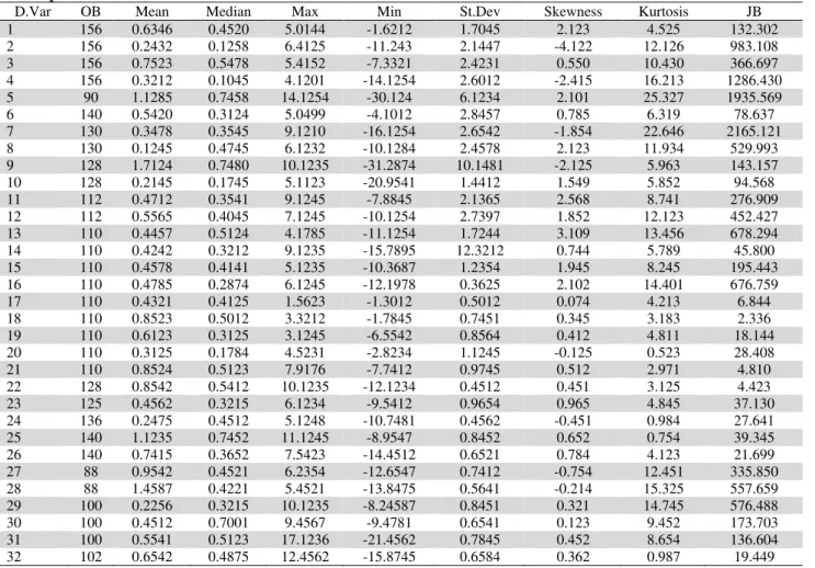
Table 1 reports the descriptive statistics of monthly return series of the individual schemes.
Table 1
Descriptive Statistics of the return series
D.Var OB Mean Median Max Min St.Dev Skewness Kurtosis JB
1 156 0.6346 0.4520 5.0144 -1.6212 1.7045 2.123 4.525 132.302
2 156 0.2432 0.1258 6.4125 -11.243 2.1447 -4.122 12.126 983.108
3 156 0.7523 0.5478 5.4152 -7.3321 2.4231 0.550 10.430 366.697
4 156 0.3212 0.1045 4.1201 -14.1254 2.6012 -2.415 16.213 1286.430
5 90 1.1285 0.7458 14.1254 -30.124 6.1234 2.101 25.327 1935.569
6 140 0.5420 0.3124 5.0499 -4.1012 2.8457 0.785 6.319 78.637
7 130 0.3478 0.3545 9.1210 -16.1254 2.6542 -1.854 22.646 2165.121
8 130 0.1245 0.4745 6.1232 -10.1284 2.4578 2.123 11.934 529.993
9 128 1.7124 0.7480 10.1235 -31.2874 10.1481 -2.125 5.963 143.157
10 128 0.2145 0.1745 5.1123 -20.9541 1.4412 1.549 5.852 94.568
11 112 0.4712 0.3541 9.1245 -7.8845 2.1365 2.568 8.741 276.909
12 112 0.5565 0.4045 7.1245 -10.1254 2.7397 1.852 12.123 452.427
13 110 0.4457 0.5124 4.1785 -11.1254 1.7244 3.109 13.456 678.294
14 110 0.4242 0.3212 9.1235 -15.7895 12.3212 0.744 5.789 45.800
15 110 0.4578 0.4141 5.1235 -10.3687 1.2354 1.945 8.245 195.443
16 110 0.4785 0.2874 6.1245 -12.1978 0.3625 2.102 14.401 676.759
17 110 0.4321 0.4125 1.5623 -1.3012 0.5012 0.074 4.213 6.844
18 110 0.8523 0.5012 3.3212 -1.7845 0.7451 0.345 3.183 2.336
19 110 0.6123 0.3125 3.1245 -6.5542 0.8564 0.412 4.811 18.144
20 110 0.3125 0.1784 4.5231 -2.8234 1.1245 -0.125 0.523 28.408
21 110 0.8524 0.5123 7.9176 -7.7412 0.9745 0.512 2.971 4.810
22 128 0.8542 0.5412 10.1235 -12.1234 0.4512 0.451 3.125 4.423
23 125 0.4562 0.3215 6.1234 -9.5412 0.9654 0.965 4.845 37.130
24 136 0.2475 0.4512 5.1248 -10.7481 0.4562 -0.451 0.984 27.641
25 140 1.1235 0.7452 11.1245 -8.9547 0.8452 0.652 0.754 39.345
26 140 0.7415 0.3652 7.5423 -14.4512 0.6521 0.784 4.123 21.699
27 88 0.9542 0.4521 6.2354 -12.6547 0.7412 -0.754 12.451 335.850
28 88 1.4587 0.4221 5.4521 -13.8475 0.5641 -0.214 15.325 557.659
29 100 0.2256 0.3215 10.1235 -8.24587 0.8451 0.321 14.745 576.488
30 100 0.4512 0.7001 9.4567 -9.4781 0.6541 0.123 9.452 173.703
31 100 0.5541 0.5123 17.1236 -21.4562 0.7845 0.452 8.654 136.604
32 102 0.6542 0.4875 12.4562 -15.8745 0.6584 0.362 0.987 19.449
* D.Var means dependent variable
The returns of all the schemes during the study period vary between -31.2874 and 17.1236. The mean returns of all the schemes are different from zero and the skewness of the distribution is also different
1 Ragnar Frish, Statistical Confluene Analysis by means of Complete Regression Systems, Institute of Economics, Oslo University, Publ. no. 5, 1934. 2Multicollinearity refers to the existence of more than one exact linear relationship and collinearity refers to the existence of a single linear relationship.
But this distinction is rarely maintained in practice and multicollinearity refers to both cases.
from zero and somewhere they indicate long left and right tails compared to the right one. On the other hand, the values of kurtosis exhibit greater than three in all respect that indicates heavy tail and the distributions of the schemes’ return series are leptokurtic. Finally, the computed J-B statistic of the individual return series of the schemes are far different from zero (J-B>0), which confirms rejection of null hypothesis that the return series are not normally distributed. Similarly, the distribution of the time series data of the independent variables is reported in Table 2.It is observed that the value of J-B statistic of the independent variables are far different from zero (J-B>0) that concludes rejection of null hypothesis under the assumption that the residuals are normally distributed.
Table 2
Summary statistics of the independent Variables
I. Var OB Mean Median Max Min St.Dev Skewness Kurtosis JB
Dy 168 1.6859 1.5641 3.1452 -8.123 0.5123 0.4125 7.123 123.758
Tb 168 0.4123 0.6654 48.1425 -28.654 6.2147 0.3214 12.125 585.751
Fl 168 2.4451 2.6412 6.1245 -21.145 3.4256 -0.7542 10.337 392.747
Ex 168 0.2324 0.6125 9.4587 -8.884 2.1478 0.6458 8.451 219.671
Rm 168 1.4745 0.9741 41.1256 -34.247 8.4712 0.5128 8.125 191.222
* I.Var means independent variable
The empirical work based on time series data assumes that the underlying time series is stationary. It is very much important that the time series data will be stationary. In short, if a time series is stationary, its mean, variance, and auto-covariance (at various lags) remain the same that means they are time invariant(Gujrati, 2007).Here, Dickey-Fuller3 (DF) test is used to measure stationarity of the time series return data.
Table 3
Unit Root test of return series of individual schemes
Sl.No Scheme Name Estimated
coefficient
Standard Error Tau (τ) Statistic DF Statistic
1 Birla India Opportunities fund-plan A (D) 0.457 0.280 4.388 -2.89 2 Birla India Opportunities fund-plan B (G) 0.142 0.173 0.421 -2.89
3 Birla MNC fund-plan A (Dividend) 0.476 0.362 1.824 -2.93
4 Birla MNC fund-plan B (Growth) -0.235 0.526 -0.453 -2.89
5 Birla Advantage fund-plan A (Dividend) 1.329 0.359 0.311 -2.93
6 Birla Advantage fund-plan B (Growth) 0.409 0.424 0.326 -2.89
7 Birla India fund-plan A (Dividend) 0.232 0.425 1.114 -2.89
8 Birla India fund-plan B (Growth) 0.243 0.261 0.372 -2.89
9 Birla Midcap fund-plan A (Dividend) 1.739 0.572 1.606 -2.89
10 Birla Midcap fund-plan B (Growth) 0.205 0.065 1.545 -2.89
11 Birla Dividend Yield Plus-Plan A (Div) 0.710 0.393 2.564 -2.89 12 Birla Dividend Yield Plus-Plan B (Growth) 0.351 0.523 0.541 -2.89
13 Birla Balance-Plan A (Dividend) 0.539 0.187 3.216 -2.89
14 Birla Balance-Plan B (Growth) 0.401 0.518 0.514 -2.89
15 Birla India Gennext Fund-Dividend option 0.345 0.241 4.527 -2.89 16 Birla India Gennext Fund-Growth option 0.423 0.184 4.423 -2.89 17 Birla Sunlife Buy India Fund-Plan A (D) 0.451 0.235 0.875 -2.89 18 Birla Sunlife Buy India Fund-Plan B (G) 0.612 0.134 4.436 -2.89 19 Birla Sunlife BasicInd India Fund-Pl A(D) 0.521 0.134 3.671 -2.89 20 Birla Sunlife Basic Ind India Fund-Pl B(G) 0.323 0.114 2.345 -2.89 21 Birla Sunlife equity fund-Plan A (Dividend) 0.604 0.138 4.201 -2.89 22 Birla Sunlife equity fund-Plan B (Growth) 0.125 0.362 1.256 -2.89 23 Birla Sunlife Frontline equity fund-Pl A (D) 0.654 0.425 3.548 -2.89 24 Birla Sunlife Frontline equity fund-Pl B (G) 0.701 0.120 2.123 -2.89 25 Birla Sunlife New Millenium fund-Pl A (D) 0.562 0.321 0.452 -2.89 26 Birla Sunlife New Millenium fund-Pl B (G) 0.456 0.145 0.652 -2.89
27 Birla Top 100-Dividend Option 0.741 0.233 -0.213 -2.89
28 Birla Top 100-Growth Option -0.123 0.102 0.236 -2.89
29 Birla Sunlife Intl equ fund Plan A D-Dir Pl 0.652 0.365 0.415 -2.89 30 Birla Sunlife Intl equ fund Plan A G-Dir Pl 0.452 0.526 0.854 -2.89 31 Birla Sunlife long term advantage-G-Dir Pl 0.632 0.421 2.412 -2.89 32 Birla Sunlife long term advantage-D-Dir Pl 0.256 0.123 6.878 -2.89
3
Dickey, D.A. & Fuller, W.A. (1979). Distribution of the estimators for autoregressive time series with a unit root.
Journal of the American Statistical Association, 74, 427-431.
586
Table 3 reports the test statistic of the of the time series data. It is observed that the computed absolute
values of the tau statistic (ǀτǀ) of eight (8) individual time series return data exceed the DF critical
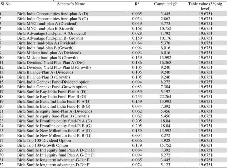
absolute tau values at 5% significance level. This means those time series data are free from unit root problem. On the other hand, in case of the remaining individual time series return data the computed absolute tau statistic are lower than the DF critical absolute tau statistics at 5% significance level, which implies the acceptance of null hypothesis. Hence, in this case, the return data are found to be non-stationary. Another problem of regression based model is heteroscedasticy. In this study, White’s heterocedastiity test is applied. Tab. 4 presents the individual regression based test statistic of heteroscedasticity. Here, the computed chi-square values of the individual regression models are lower than the critical chi-square value at 5% level of significance and hence, it may be argued that there is absence of heteroscedasticity in the regression models.
Table 4
Test of Heteroscedasticity
Sl.No Scheme’s Name R2 Computed χ2 Table value (5% sig.
level)
1 Birla India Opportunities fund-plan A (D) 0.065 3.445 19.6751
2 Birla India Opportunities fund-plan B (G) 0.054 2.862 19.6751
3 Birla MNC fund-plan A (Dividend) 0.049 3.773 19.6751
4 Birla MNC fund-plan B (Growth) 0.168 10.752 19.6751
5 Birla Advantage fund-plan A (Dividend) 0.028 1.792 19.6751
6 Birla Advantage fund-plan B (Growth) 0.159 10.176 19.6751
7 Birla India fund-plan A (Dividend) 0.084 5.376 19.6751
8 Birla India fund-plan B (Growth) 0.094 6.016 19.6751
9 Birla Midcap fund-plan A (Dividend) 0.094 6.016 19.6751
10 Birla Midcap fund-plan B (Growth) 0.159 13.992 19.6751
11 Birla Dividend Yield Plus-Plan A (Div) 0.186 16.368 19.6751
12 Birla Dividend Yield Plus-Plan B (Growth) 0.105 9.240 19.6751
13 Birla Balance-Plan A (Dividend) 0.105 9.240 19.6751
14 Birla Balance-Plan B (Growth) 0.105 9.240 19.6751
15 Birla India Gennext Fund-Dividend option 0.094 8.272 19.6751
16 Birla India Gennext Fund-Growth option 0.083 7.304 19.6751
17 Birla Sunlife Buy India Fund-Plan A (D) 0.059 5.192 19.6751
18 Birla Sunlife Buy India Fund-Plan B (G) 0.253 22.264 19.6751
19 Birla Sunlife Basic Ind India Fund-Pl A(D) 0.159 13.992 19.6751
20 Birla Sunlife Basic Ind India Fund-Pl B(G) 0.084 7.392 19.6751
21 Birla Sunlife equity fund-Plan A (Dividend) 0.062 5.456 19.6751
22 Birla Sunlife equity fund-Plan B (Growth) 0.062 5.456 19.6751
23 Birla Sunlife Frontline equity fund-Pl A (D) 0.205 18.04 19.6751
24 Birla Sunlife Frontline equity fund-Pl B (G) 0.205 18.04 19.6751
25 Birla Sunlife New Millenium fund-Pl A (D) 0.159 13.992 19.6751
26 Birla Sunlife New Millenium fund-Pl B (G) 0.094 8.272 19.6751
27 Birla Top 100-Dividend Option 0.056 4.928 19.6751
28 Birla Top 100-Growth Option 0.179 15.752 19.6751
29 Birla Sunlife Intl equity fund Plan A D-Dir Pl 0.084 7.392 19.6751
30 Birla Sunlife Intl equity fund Plan A G-Dir Pl 0.094 8.272 19.6751
31 Birla Sunlife long term advantage-G-Dir Pl 0.065 3.445 19.6751
32 Birla Sunlife long term advantage-D-Dir Pl 0.074 5.123 19.6751
multicolinearity problem. Here, the computed tolerance value ranges between 0.302 and 0.745 which clearly indicates that the individual regression models are free from the problem of multicolinearity. Here, the results of R2, VIF and TOL are discussed but the values are not presented here.
Table 4
Test of Multicolinearity (Pearson Correlation matrix)
Variable Rm DY TB FL EX
Rm 1.000
DY 0.1235 1.000
TB -0.0546 -0.1425 1.000
FL -0.2014 -0.2054 0.1845 1.000
EX -0.2541 -0.0674 0.0541 0.2145 1.000
If we look back in Table 1, we observe that the average monthly return performance of the schemes is positive. Generally, the return performance is influenced by two reasons one is managers’ abilities to select the under priced securities (stock-selection) and the other is to predict the market movement correctly (market-timing). Although, the prediction of security prices is not an easy task that requires efficiency of the fund managers to analysis of under-valued and over-valued security prices judiciously that ensure higher return. It is generally expected that positive alpha value (a measure of stock-selection) represents manger’s ability to select right stocks that finally add value to the mutual fund portfolios. Similarly, significant positive alpha indicates managers are superior to select under priced securities, which finally add extra value to the mutual fund portfolios. If we look back to the past studies on selectivity performance of the managers we can see a mix results like positive, negative and superior performances.
Table 6
Estimation of selectivity performance based onunconditional measure
Sl.No Scheme’s Name Alpha t-value D-W
1 Birla India Opportunities fund-plan A (D) 0.530 3.542* 1.632
2 Birla India Opportunities fund-plan B (G) 0.458 0.269 1.543
3 Birla MNC fund-plan A (Dividend) 0.754 2.254* 1.815
4 Birla MNC fund-plan B (Growth) 0.574 0.761 2.004
5 Birla Advantage fund-plan A (Dividend) 1.412 3.129* 1.546
6 Birla Advantage fund-plan B (Growth) 0.402 2.132* 1.795
7 Birla India fund-plan A (Dividend) 0.345 0.593 1.946
8 Birla India fund-plan B (Growth) -0.074 -0.149 1.451
9 Birla Midcap fund-plan A (Dividend) 2.123 1.993* 2.104
10 Birla Midcap fund-plan B (Growth) 0.089 1.012 1.802
11 Birla Dividend Yield Plus-Plan A (Div) 0.510 0.817 1.854
12 Birla Dividend Yield Plus-Plan B (Growth) 0.475 0.942 1.740
13 Birla Balance-Plan A (Dividend) 0.514 2.203* 1.541
14 Birla Balance-Plan B (Growth) -0.042 -0.512 2.120
15 Birla India Gennext Fund-Dividend option 0.602 0.201 1.562
16 Birla India Gennext Fund-Growth option 0.415 1.574 1.841
17 Birla Sunlife Buy India Fund-Plan A (D) 0.462 2.323* 1.754
18 Birla Sunlife Buy India Fund-Plan B (G) 0.612 0.226 1.603
19 Birla Sunlife Basic Industries India Fund-Pl A(D) 0.665 3.126* 1.704
20 Birla Sunlife Basic Industries India Fund-Pl B(G) -0.302 -0.541 1.565
21 Birla Sunlife Equity fund-Plan A (Dividend) 0.701 0.283 1.901
22 Birla Sunlife Equity fund-Plan B (Growth) 0.512 0.812 1.412
23 Birla Sunlife Frontline equity fund-Pl A (D) 0.624 1.978* 1.621
24 Birla Sunlife Frontline equity fund-Pl B (G) -0.012 -0.602 1.874
25 Birla Sunlife New Millenium fund-Pl A (D) 1.502 2.201* 1.624
26 Birla Sunlife New Millenium fund-Pl B (G) 1.355 1.213 1.804
27 Birla Top 100-Dividend Option 0.328 2.102* 1.975
28 Birla Top 100-Growth Option -0.102 -0.325 2.010
29 Birla Sunlife Intl equity fund Plan A D-Dir Plan 0.648 2.025* 1.754
30 Birla Sunlife Intl equity fund Plan A G-Dir Plan 0.503 0.723 1.665
31 Birla Sunlife long term advantage-G-Dir Plan 1.244 1.932 1.998
32 Birla Sunlife long term advantage-D-Dir Plan 0.012 0.557 2.321
588
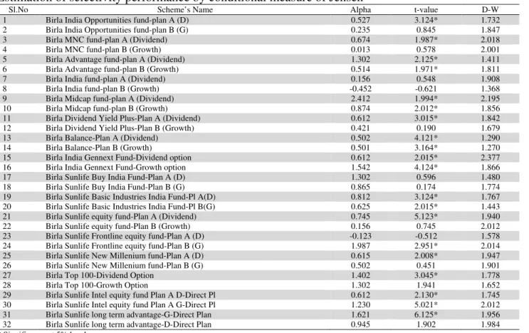
The stock-selection performance based on unconditional model is given in Table 6.It is observed that the alpha values of 27 schemes are positive and the remaining is negative. Here, the probable reason for obtaining negative alpha may be caused for the inability of the managers’ to select the under-priced securities correctly. The positive performance may be considered due to the managers’ ability to predict the security prices correctly. Moreover, fund managers produce significant alpha by applying their skills on stock-selection activities from the volatile market. It is observed from the table that the alpha values of twelve (12) schemes are statistically significant at 5% level. In that case, only 37.5% managers of the sample schemes are superior stock pickers who correctly selected the under-priced securities and finally add additional returns to the portfolios. Although, the selectivity performance is not satisfactory. Table 6 also presents the test statistic of autocorrelation. Here, Durbin-Watson (1951) test is applied. Accordingly, if the value of ‘d’ is two, one may assume that there is no first-order autocorrelation in the regression model. The observed ‘d’ values of majority of the schemes are far less than 2 and hence, the return data are free from first order autocorrelation. Finally, the stock-selection performance based on conditional measure is presented in Table 7. It is observed that the estimated conditional alpha values (a measure of conditional selectivity performance) of two schemes are negative and the remaining schemes have positive. The observed positive selectivity performances of the two measures are quite same and the difference observed is negligible. It is also found that twenty (20) schemes have provided significant stock-selection performances out of thirty two (32) schemes. If we compare the significant stock-selection performance based on two measures we find that conditional model is better. According to the unconditional model, the number of significant stock-selection performers is twelve (12) where as in conditional model the number is twenty (20) or in percentages the former is 37.5% and the latter is 62.5%. Therefore, we can conclude that inclusion of public information variables in the conditional model generate better performance estimates in Indian context based on sample schemes. Here, the computed test statistic is 2.012, which is higher than the table value of z at 5% level (1.96) of significance. This prompts us to reject the null hypothesis and concluded conditional stock selection performance is superior to traditional performance measure.
Table 7
Estimation of selectivity performance by conditional measure of Jensen
Sl.No Scheme’s Name Alpha t-value D-W
1 Birla India Opportunities fund-plan A (D) 0.527 3.124* 1.732
2 Birla India Opportunities fund-plan B (G) 0.235 0.845 1.847
3 Birla MNC fund-plan A (Dividend) 0.674 1.987* 2.018
4 Birla MNC fund-plan B (Growth) 0.013 0.578 2.001
5 Birla Advantage fund-plan A (Dividend) 1.302 2.125* 1.411
6 Birla Advantage fund-plan B (Growth) 0.514 1.971* 1.811
7 Birla India fund-plan A (Dividend) 0.156 0.548 1.908
8 Birla India fund-plan B (Growth) -0.452 -0.621 1.368
9 Birla Midcap fund-plan A (Dividend) 2.412 1.994* 2.195
10 Birla Midcap fund-plan B (Growth) 0.874 2.012* 1.856
11 Birla Dividend Yield Plus-Plan A (Dividend) 0.612 3.015* 1.842
12 Birla Dividend Yield Plus-Plan B (Growth) 0.421 0.190 1.679
13 Birla Balance-Plan A (Dividend) 0.502 4.121* 1.290
14 Birla Balance-Plan B (Growth) 0.501 3.164* 1.270
15 Birla India Gennext Fund-Dividend option 0.612 2.015* 2.377
16 Birla India Gennext Fund-Growth option 1.542 4.124* 1.866
17 Birla Sunlife Buy India Fund-Plan A (D) 1.302 0.596 1.480
18 Birla Sunlife Buy India Fund-Plan B (G) 0.865 0.174 1.774
19 Birla Sunlife Basic Industries India Fund-Pl A(D) 0.812 3.124* 1.767 20 Birla Sunlife Basic Industries India Fund-Pl B(G) 0.625 2.015* 1.443 21 Birla Sunlife equity fund-Plan A (Dividend) 0.745 5.123* 1.940
22 Birla Sunlife equity fund-Plan B (Growth) 0.156 0.745 2.012
23 Birla Sunlife Frontline equity fund-Plan A (D) -0.123 -0.512 1.578 24 Birla Sunlife Frontline equity fund-Plan B (G) 1.987 2.951* 2.014 25 Birla Sunlife New Millenium fund-Plan A (D) 0.615 2.008* 1.947 26 Birla Sunlife New Millenium fund-Plan B (G) 0.502 0.451 1.901
27 Birla Top 100-Dividend Option 1.402 3.045* 1.778
28 Birla Top 100-Growth Option 1.302 1.941 1.652
7. Conclusion
Before the development of the conditional model traditional measures are extensively used in investment performances. With the growing popularity of conditional measure, a new age is opened in the investment performance. In the present study, it is observed that the superior selectivity performance of the sample schemes based on traditional measure is not satisfactory. But, incorporation of available public information variables in the traditional measure the significant stock-selection performances of the managers have been radically changed. In this model the statistically significant stock-selection performance is increased to twenty (20) from twelve (12). Our evidences agree with the earlier views that after inclusion of public information variables in the conditional model, the selection performance confirms better. The statistical test also reveals that the conditional stock-selection performance of the sample schemes of Birla Sun Life Mutual Fund Company is better than traditional measure. In addition to this, the uses of multi-index multi-factor conditional measures and along with this sustainable investment performance are the natural extension of this paper particularly in Indian context.
References
Arditti, F. D. (1971). Another look at mutual fund performance. Journal of Financial and Quantitative
Analysis, 6(03), 909-912.
Artikis, G. (2004). Bond mutual fund managers’ performance in Greece. Journal of Managerial Finance, 30(10), 1-6.
Athanassakos, G., Carayannopoulos, P., & Racine, M. (2002). How effective is Aggressive Portfolio Management. Canadian Investment Review, 15(3), 39-44.
Chander, R. (2005). Empirical Investigation on the Investment Managers’ Stock Selection Abilities: The Indian Experience. The ICFAI Journal of Applied Finance, 11(7), 5-20.
Coggin, T. D., Fabozzi, F. J., & Rahman, S. (1993). The investment performance of US equity pension fund managers: An empirical investigation. The Journal of Finance, 48(3), 1039-1055.
Chang, E. C., & Lewellen, W. G. (1984). Market timing and mutual fund investment performance. Journal of
Business, 57(1), 57-72.
Christopherson, J. A., Ferson, W. E., & Glassman, D. A. (1998). Conditioning manager alphas on economic information: Another look at the persistence of performance. Review of Financial Studies, 11(1), 111-142. Christopherson, J. A., Ferson, W. E., & Turner, A. L. (1999). Performance evaluation using conditional alphas
and betas. The Journal of Portfolio Management, 26(1), 59-72.
Chen, Z., & Knez, P. J. (1996). Portfolio performance measurement: Theory and applications. Review of
Financial Studies, 9(2), 511-555.
Dybvig, P. H., & Ross, S. A. (1985). Differential information and performance measurement using a security market line. The Journal of finance, 40(2), 383-399.
Drew, M. E., Veeraraghavan, M., & Wilson, V. (2005). Market timing, selectivity and alpha generation: evidence from Australian equity superannuation funds. Investment Management and Financial Innovations,2(2), 111-127.
Fama, E. F. (1972). Components of investment performance. The Journal of finance, 27(3), 551-568.
Ferson, W. E., &Schadt, R. W. (1996). Measuring fund strategy and performance in changing economic conditions. The Journal of Finance, 51(2), 425-461.
Fama, E. F., & French, K. R. (1989). Business conditions and expected returns on stocks and bonds. Journal of
financial economics, 25(1), 23-49.
Fransworth, H. (1997). Conditional performance Evaluation. In paxson, D., Wood, D. (eds), Blackwell Encyclopedic Dictionary of Finance, Blackwell Business, 23-24.
Ferson, W. E., & Warther, V. A. (1996). Evaluating fund performance in a dynamic market. Financial Analysts
Journal, 52(6), 20-28.
Ferson, W., & Qian, M. (2004). Conditional performance evaluation, revisited, Working Paper, Boston College-EUA.
Grinblatt, M., & Titman, S. (1989). Portfolio performance evaluation: Old issues and new insights. Review of
590
Grant, D. (1977). Portfolio performance and the “cost” of timing decisions. The Journal of Finance, 32(3), 837-846.
Gordon, M.J., & Gangoli, R. (1962). Choice among and scale of play on lottery type alternatives. College of Business Administration, University of Rochester, pp. 1-25.
Graham, J. R., & Harvey, C. R. (1996). Market timing ability and volatility implied in investment newsletters' asset allocation recommendations. Journal of Financial Economics, 42(3), 397-421.
Hicks, J. R. (1962). Liquidity. The Economic Journal, 72(288), 787-802.
Henriksson, R. D., & Merton, R. C. (1981). On market timing and investment performance. II. Statistical procedures for evaluating forecasting skills. Journal of business, 44, 513-533.
Ilmanen, A. (1995). Time‐Varying Expected Returns in International Bond Markets. The Journal of
Finance, 50(2), 481-506.
Iqbal.,&Quader. (2012). Survivorship-biased free mutual funds in Pakistan. American Journal of Scientific Research, 62, 127-134.
Jensen, M. C. (1968). The performance of mutual funds in the period 1945-1964.The Journal of Finance, 23, 389-416.
Jensen, M. (1972). Optimal utilization of market forecasts and the evaluation of investment performance. In Szego, G; Shell, K. (eds), Mathematical methods in Investment and Finance, North-Holland, 310-335. Kader, M., & Kuang, Y. (2007). Risk-adjusted performance, selectivity, timing ability and performance
persistence of Hong Kong mutual funds. Journal of Asia-Pacific Business, 8(2), 25-28.
Kon, S. J., & Jen, F. C. (1979). The investment performance of mutual funds: An empirical investigation of timing, selectivity, and market efficiency. Journal of Business, 52, 263-289.
Kosowski, R., Timmermann, A., Wermers, R., & White, H. (2006). Can mutual fund “stars” really pick stocks? New evidence from a bootstrap analysis. The Journal of finance, 61(6), 2551-2595.
Koulis, A., Beneki, C., Adam, M., & Botsaris, C. (2011). An Assessment of the Performance of Greek Mutual Equity Funds Selectivity and Market Timing. Applied Mathematical Sciences, 5(4), 159-171.
Lintner, J. (1965). Security Prices, Risk, and Maximal Gains from Diversification*. The Journal of
Finance, 20(4), 587-615.
Lee, C. F., & Rahman, S. (1990). Market timing, selectivity, and mutual fund performance: An empirical investigation. Journal of Business, 63, 261-278.
Mossin, J. (1966). Equilibrium in a capital asset market. Econometrica: Journal of the econometric society, 34, 768-783.
Markowitz, H. M. (1952). Portfolio selection. Journal of Finance, 12, 77-91.
Mansor, F., & Bhatti, M. I. (2011, February). The Islamic mutual fund performance: New evidence on market timing and stock selectivity. In 2011 International Conference on Economics and Finance Research
IPEDR (Vol. 4).
Otten, R., & Bams, D. (2004). How to measure mutual fund performance: economic versus statistical relevance. Accounting & finance, 44(2), 203-222.
Pesaran, M. H., & Timmermann, A. (1995). Predictability of stock returns: Robustness and economic significance. The Journal of Finance, 50(4), 1201-1228.
Redman, A. L., Gullett, N. S., & Manakyan, H. (2000). The performance of global and international mutual funds. Journal of Financial and strategic Decisions, 13(1), 75-85.
Roy, S., & Ghosh, S. K. (2012). Selectivity as a measure of mutual fund performance: A comparative study of the open-ended income and growth schemes. Global Journal of Finance and Economic Management, 1(1), 69-86.
Sharpe, W. F. (1963). A simplified model for portfolio analysis. Management science, 9(2), 277-293.
Sharpe, W. F. (1966). Mutual fund performance. Journal of Business, 39, 119-138.
Silva, F., Cortez, M. D. C., & Armada, M. R. (2003). Conditioning information and European bond fund performance. European Financial Management, 9(2), 201-230.
Sondhi, H. J., & Jain, P. K. (2006). Can Growth Stocks be identified for Investment? A Study of Equity Selectivity Abilities of Fund Managers in India. The ICFAI Journal of Applied Finance, 12(2), 6-17.
Sipra, N. (2002). Mutual fund performance in Pakistan 1995-2004.www.ssrn.com, pp. 6-45.
Shanmughan., & Zabiulla. (2011). Stock selection strategies of equity mutual fund managers in India. Middle Eastern Finance and Economics, 11, 19-27.
Treynor, J. L. (1965). How to rate management of investment funds. Harvard business review, 43(1), 63-75.
Treynor, J. L., &Mazuy, J. (1966). Can mutual fund outguess the market. Harvard Business Review, 43(1), 63-75.