A Work Project presented as part of the requirements for the Award of a Masters Degree in
Finance from the Nova School of Business and Economics.
BOND FUND RUNS: THE FINANCIAL CRISIS CASE
Ana Catarina Leitão Afonso
Student Number 541
A project carried out on the Financial Markets major, under the supervision of:
Professor Miguel Ferreira
Abstract
This paper studies the monthly flows of bond fund geographically focused on Europe and on the
United States in the period between 2002 and 2012, with special attention to the effect of the
financial crisis of 2008. Through the usage of the panel quantile regression model, this study aims
to identify which funds, in terms of their characteristics, are more likely to suffer a run. The main
finding is that the impact of the characteristics of fund flows is not equal for all funds, varying with
issuer entity, the state of the economy as well as the focus of the fund. During the financial crisis,
runs were more pronounced, situation that still affects funds geographically focused on Europe.
Keywords: Runs; Liquidity crisis; Vector Autoregression; Quantile Regressions.
Acknowledgements
I am grateful to every member of the educational system that took part in my academic
growth. Sónia Félix and Marta Lopes for the help with the initial support programming
and especially Professor Miguel Ferreira for the invaluable guidance during the
development period of the presented study.
1. Introduction
Since the global financial crisis in 2008, the global economy has experienced a slow growth,
which exposed the unsustainable fiscal policies of many countries around the world namely in
Europe. This debt crisis had and still has a negative impact on the global financial markets, where
investors’ reactions to any bad news coming were fast, leading, in most of the times, to runs of all
types of securities and funds.
Nowadays, this is one of the most important problems affecting the world economy and, until
now, with no end in sight. This is a crisis that is considered by many economists as the worst after
the economic depression that also emerged in the United States at the end of 1920’s: The Great
Depression of 1929. At that time, the desire to misallocate funds was greater, especially in banks
where depositors withdraw their deposits from banks for the fear of the safety of their money.
Therefore, runs are a phenomenon that can largely be explained by investors’ actions and its
empirical evidence started a long time ago. Diamond and Dybvig (1983) is one of the most
important literature references about runs that tries to explain how runs propagate in our society,
focusing on the problem of the maturity transformation and its relation with the investors’ actions.
Another important theory, developed by Jacklin and Bhattacharya (1988), is based on the
relationship between insolvent banks and runs.
In this paper, I study runs on bond funds in the period between 2002 and 2012, with special focus
on the financial crisis of 2008. Bond funds are not all equal, they have their own characteristics that
should be taken into account. This study will also be focused on both Sovereign and Corporate bond
funds, more specifically on the impact that each bond issuer type has on fund runs, its determinants
and how that is linked to the country’s credit rating. Though, the goal of this study is to identify
which funds, in terms of their characteristics, are more likely to suffer a run.
I use monthly flows of bond funds between 2002 and 2012, geographically focused on the
as well as, the country credit rating. At the end, I will determine which funds’ characteristics are the
most significant to explain funds flow. To conduct this analysis, I use a panel quantile regression
model to better account for the shape of the flows distribution, as well as for the characteristics of
fund flows. It is shown that during the financial crisis period runs are more pronounced than in the
remaining periods, although, more recently, there are some significant outflows, namely for Europe.
Regarding the characteristics of funds, higher funds return tend to have larger outflows and inflows
in the left and right tails, respectively, until the crisis period for corporate funds. After crisis, older
corporate funds with higher returns tend to have lower outflows in the left tail in the US, but larger
outflows in the same tail in Europe. For sovereign funds, before crisis, in the US, the ones with
higher TER and owned by institutional investors tend to have low outflows in the left tail, similarly
to what happen in Europe in the right tail. During the crisis period, in both regions, funds with higher
returns and owned by institutional investors face larger outflows both in the left and right tails. After
crisis, large-scale funds have large outflows in the right tail, with institutional investors having lower
outflows in the left tail. As a consequence, the impact of the characteristics of fund flows is not equal
for all funds, it varies with issuer entity, the state of the economy as well as the focus of the fund.
The remainder paper proceeds as follows1. Section 2 describes the importance of bond funds in the United States and Europe, while in Section 3 it is provided a short literature review on runs.
Section 4 focuses on the used data set of this empirical study. In Section 5 it is discussed the
methodology, whereas in Section 6 it presents the empirical results. Section 7 concludes the study.
2. The importance of Bond funds in the US and Europe
Globalisation is a set of transformations in the global political and economic orders that has been
gaining importance since the end of the twentieth century, especially in what concerns to bond
1This study contains 25 pages (pp. 1-25). The appendices pages (pp. 26-33) are a complement of the content presented in the main
markets. Although US has traditionally dominated the world’s bond markets, European bond
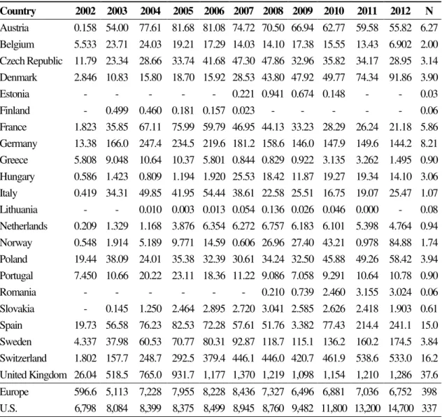
market is now trying to reverse the past history. Table 1 presents the yearly number of Total Net
Assets (TNA) of the funds only for the regions under analysis (Europe and the US) until the end of
20122. TNA is defined as the sum of all total fund value (in $ million). TNA have mostly been
showing an increasing tendency since 2002, evidencing the increase popularity of bond funds. The
exception years are from 2007 to 2009, when the total net assets of funds with geographic
investment focus on Europe and the US presented a decrease of almost $1.5 million. This is a
decrease that can be easily explained by the liquidity crisis that started affecting both regions in
2007, causing significant reduction to the value of this type of funds. Specifically, this reduction was
more pronounced among European countries, namely Portugal, Spain, Italy and France, countries
that on average suffer more with the liquidity crisis. After 2009, TNA of European and American
bond funds totalled $60.4 million, of which 66% were geographically focused on the US continent.
Regarding European countries, Greece was the one that significantly underperformed the European
average by presenting a decrease of 52% after 2009.
Table 1:Yearly Number of Total Net Assets (partial)
Region 2002 2003 2004 2005 2006 2007 2008 2009 2010 2011 2012 N Europe 597 5,113 7,228 7,955 8,228 8,436 7,327 6,496 6,881 7,036 6,752 398 U.S. 6,798 8,084 8,399 8,375 8,499 8,945 8,760 9,482 11,800 13,200 14,700 337
Note: The presented numbers are in thousands.
3. Literature Review
Fund Runs are events that have been studied for a long time. One of the most important literature
references about runs tries to explain how runs propagate in our society. Through a careful
description and analysis, Diamond and Dybvig (1983) (hereafter: DD) constructed a model that
analyses the problem of maturity transformation in bank runs in the real economy taking into
consideration the relation between the economics of banking and policies’ issues. In their
equilibrium, they find that financing bank’s long-terms loans with short-term deposits can lead to
bank runs, since some later depositors withdraw their deposits because of their sense of panic that
other late depositors also would withdraw, causing a snow-ball effect that would then result in a
possible bank failing. Another important finding of the author is related with deposits’ insurance
with which the government intervention can eliminate the runs.
Jackelin (1987) used the DD model assumptions to understand what would happen with firms,
but instead of using insurance financed by taxes, the author uses dividends and shares, achieving a
different equilibrium from DD’s one. In his equilibrium, consumers can trade dividends for firm’s
shares, by giving the option for late consumers to invest their dividends by buying shares at market
price, the same shares that early consumers sold after obtaining their dividends, eliminating the
possibility of occurrence of a run. Gorton and Pennacchi (1993) try to give a solution for this
problem that arises from the maturity gap, proposing the elimination of this gap with narrow banks
leaning on short-term securities, which would avoid bank runs.
Another common feature in most of the runs’ studies is the relation between funds persistent
performance and runs. Brown, Goetzmann, Ibbotson and Ross (1992) used a non-parametric
method to study the relation between past and future mutual fund performances. They present
numerical examples favoring the evidence of predictable returns between past and future
performance in mutual funds. Other important reference on performance and runs is the one from
Chen, Goldstein and Jiang (2010) that empirically studied the relationship between payoff
complementaries and financial fragility concerning mutual fund outflows. According to this study,
illiquid funds tend to have stronger payoff complementaries and, consequently, the outflows are
more sensitive to bad performance, a situation that is more common in funds held by retail investors.
More recently, Schmidt et al. (2013) studied daily investor flows to and from individual money
models, the authors found that outflows were more concentrated in funds with lower liquidity
among institutional investors that moved their money mostly from Commercial Papers into U.S.
government’s funds.
European literature on runs is very scarce when compared to the American one. Jank and
Wedow (2010) investigated the returns and flows of German money market funds over the period
of 1996-2008. The main conclusion of the paper is that in liquid times some money market funds’
managers enhanced their returns by investing in less liquid assets, outperforming other funds as long
as liquidity in the market was high. However, during the liquidity crisis of 2007/2008, illiquid funds
experienced runs.
4. Data and initial results
4.1. Sample, Data and Descriptive Statistics
The initial sample includes 70,688 bond funds from 2002 to 2012 collected from the Lipper
database. Exchange listed, index-tracking, funds-of-funds and close-end funds were eliminated, as
well as funds that were not considered as primary ones, reducing the initial sample to 25,083 bond
funds. The fund investment can have different focus which is based on the Lipper geographic focus
and it can be a single country, a geographic region or the global one. In order to better organize the
sample, five regions are created: Asia-Pacific, Emerging Markets, Europe, Global and North
America (hereafter: US), but only the Europe and United States ones are used in this analysis.
Monthly data is used to better analyse both retail and institutional investors’ actions across the
sample period. In what concerns to the bond issuer, the data set is divided between Sovereign funds
and Corporate ones. The variables are then winsorized at the bottom and top in 1% to eliminate
extreme outliers of the sample3.
Because bond funds are not all equal it is important to identify the main variables that had a
major impact on current fund flows. Control variables include lagged flow (𝐿𝑎𝑔𝐹𝑙𝑜𝑤), total
expense ratio (𝑇𝐸𝑅), flow standard deviation (𝐹𝑙𝑜𝑤 𝑆. 𝐷.), the logarithm of total net assets (𝑆𝑖𝑧𝑒),
the cumulative flow (𝐶𝑓𝑙𝑜𝑤), the total load (𝐿𝑜𝑎𝑑), fund age (𝐴𝑔𝑒), the lagged return (𝐿𝑎𝑔𝑅𝑒𝑡)
and a dummy variable for the bond issuer type (𝐵𝑒𝑛𝑐ℎ𝑚𝑎𝑟𝑘). Table A.2 in the appendix provides
the descriptive statistics of the stated variables for Europe (panel A) and the US (panel B) regions.
4.2.Fund Flows
One of the main variables of this study is the fund net flow (Flow). 𝐹𝑙𝑜𝑤𝑖𝑡is defined as the net
growth in TNA of the fund 𝑖 in the month 𝑡, assuming that flows occur at the end of each month:
𝐹𝑙𝑜𝑤𝑖𝑡 = 𝑇𝑁𝐴𝑖𝑡−𝑇𝑁𝐴𝑇𝑁𝐴𝑖𝑡−1𝑖𝑡−1(1+𝑅𝑒𝑡𝑖𝑡), (1)
where 𝑇𝑁𝐴𝑖𝑡 is the total net asset value of each fund 𝑖 (in $ Million) at the end of the month 𝑡, and
𝑅𝑒𝑡𝑖𝑡 is the fund 𝑖 raw return in month 𝑡. Table A.4 of the appendix shows descriptive statistics of
fund flows until December of 2012. Specifically, the mean, standard deviation and a range of
quantiles during the sample period are presented for each European country and for the US.
Through the analysis of the table, we conclude that the average flow from 2002 to 2012 is, in the
majority of the countries, nearly zero. It is also interesting to notice that, although the US have a
longer history with bond funds, between 2002 and 2012, the number of funds geographically
focused on Europe are higher than the ones geographically focused on the US.
4.3.Flow distribution
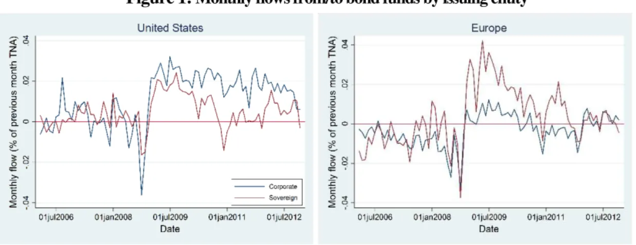
Figure 1 shows the monthly aggregated flows as a percentage of total assets of both issuing
entities to the US (panel A) and Europe (panel B) regions between 2006 and 20124.
4Note that, because this is a set of funds with geographic focus in the US and Europe, it does not mean that all
Figure 1: Monthly flows from/to bond funds by issuing entity
Panel A: United States monthly funds Panel B: European monthly flows
Depending on the time, the risk associated with each individual (corporate and sovereign) fund
varies implying decisive changes in funds’ flows. Considering the US case, corporate funds had
higher outflows than the sovereign ones during the peak of the liquidity crisis of 2008. More
specifically, corporate funds presented a maximum outflow of 3.6% in October 2008, the same
month in which sovereign funds also achieved their maximum outflow, of 1.6%. After that month,
both types of funds showed a good recovery, specially the corporate ones that in July 2009 presented
inflows of 3.2%, similarly to what happened to sovereign funds that also had a good rebound in
2009, by achieving inflows of almost 2.5% in September of that year. This sovereign decrease in
2010 can be seen as the reflex of investors’ fear due to the American midterm elections of
November 2010, where the Republicans regained the control of the chamber.
European funds’ behaviour is somehow related with the US funds’ one. Once the US dominates
the world’s bond markets, a negative impact in the US economy can have consequences all over
the world. The collapse of Lehman Brothers in 2008 strongly affected Europe since many of the
European countries had funds in dollar currency and experienced large outflows. Like what
happened with the US funds in 2008, European geographically focused funds also had the largest
outflows since 2006. However, contrarily to the US, in Europe, sovereign funds were the ones that
showed the largest outflows, with a maximum of more than 3.7% in October of 2008, against the
inflows, although the sovereign ones performed better and earlier, achieving a maximum inflow of
4.2% in May, in contrast to the 1.2% accomplishing by corporate funds in July.
We can easily see that Europe and the US differ in time and in issuing entities’ runs. In the
former, since mid-2008, corporate funds tend to underperform the sovereign ones, contrarily to what
happens in the US, where corporate funds tend to outperform the sovereign ones, in the sense that,
in Europe, corporate funds tend to have lower inflows and larger outflows than sovereign funds, in
opposition to what happens in the US. Note that, in Europe most of the companies are facing
financial problems which makes them less appellative for investors and therefore their bond funds
face higher outflows. However, for the US, the empirical evidence is the opposite. Because
American companies tend to be more financially stable, investors tend to put more of their effort
into corporate funds resulting in higher inflows than for sovereign funds. Regarding the time,
Europe presented less stability of flows than the US after the peak of 2008, situation that can be
explained by the financial difficulties that some of the European countries have constantly been
facing since the emergence of the liquidity crisis.
It is also interesting to view what happened in some European countries, namely the comparison
between those that have been facing higher financial problems (such as Portugal and Greece) and
those that are considered financially stable (such as Germany and Austria). Note that Austria and
Germany are countries financially stable, with higher credit ratings than Greece or Portugal. More
specifically, according to Standard and Poor’s(thereafter: S&P) and Moody’s, both Austria and
Germany had the highest credit rating possible until the beginning of 2012: AAA and Aaa,
respectively given by S&P and Moody’s5. Regarding Portugal and Greece, the story is much
different. Considering only the period between 2002 and 2012, Portugal credit rating had six
5 Thereafter, it will only be stated S&P downgrades/upgrades to avoid repeated information, since Moody’s downgrades/upgrades
consecutive downgrades from AA in 2004 to BB in 2012, much better than the Greek situation that
on the same period had eight consecutive downgrades, from A+ in 2003 to CCC in 2012.
Due to all these changes, it is important to check if a country credit rating is somehow linked to
funds outflows. Figure 2 shows the monthly aggregated flows as a percentage change of total assets
for Austria (top left panel), Germany (top right panel), Greece (bottom left panel) and Portugal
(bottom right panel). Focusing on the top panel of figure 2, we see that, although Austria and
Germany are stable countries, they also tend to have outflows both in corporate and sovereign funds,
especially in corporate funds. More specifically, Austria and Germany had a large corporate outflow
in mid-2009 that, in Austria, was rapidly compensated by an inflow on the same type of funds
months later. Note that the largest outflows and inflows occurred in corporate funds. Sovereign
funds also presented months with outflows, but their magnitude was much lower.
If we now focus on the bottom panel, we see that sovereign funds in Greece and Portugal are
relatively more recent than the corporate’s. However, that fact does not prevent outflows in these
countries. More specifically, Greece had large outflows at the end of 2010, contrarily to what
happened in Portugal that registered a large inflow at the beginning of 2011, followed then by an
equivalent outflow. Regarding the corporate funds, Greece flows alternated between in and
outflows with the largest inflow magnitude in July 2009. For Portugal, corporate funds also alternate
between in and outflows, but with lower magnitude than in Greece. Therefore, a country credit
Figure 2 - Monthly flows from/to Austria, Germany, Greece and Portugal
To get a better picture and a more comprehensive analysis of the extremes situations that
happened in the bond funds markets, we should look at the tails of the flow distribution of both
regions. More precisely, the percentage outflows of the 10th, 50th (median) and 90th quantiles of funds were studied and the results are presented in figure A.1 of the appendix. Starting with the
corporate funds, in Europe (left panel A) the vertical distance between the 10th and 90th quantiles varied across the years. The widest distance was at the time of the emergence of the liquidity crisis,
where it was verified the largest outflows in all tails of the distribution. Regarding the median,
beyond the outflow in 2008, it had a slightly inflow at the beginning of 2011, that also reached the
right tail of the distribution, contrarily to what happened to the left tail, that has been experiencing
outflows since mid-2011. Like what happened in Europe, in the US (right panel A) the widest
vertical distance between the right and left tails occurred in 2008, when all the tails suffered the
largest outflows. After that year the median tended to be stable, contrary to what happened with the
Regarding the sovereign funds, Europe (left panel B) presents a wide vertical distance between
right and left tails than the US (right panel B). In the former, this vertical distance increased
significantly in 2008, keeping unstable and with an increase trend until 2011, when the left tail
presented a larger outflow than the right tail. The median was stable during all periods, except for
the emergence of the financial crisis and in 2011, when it experienced a slight outflow. In the US
the more pronounced vertical difference occurred, once again, during the liquidity crisis’ peak. From
then on, there were some instability both on right and left tails, but its vertical distance became tight,
compared to what happened in Europe.
Therefore, it is possible to conclude that there is heterogeneity in the behaviour of European and
the US’ fund flows, independently from the issue entity. This heterogeneity is specially pronounced
at the time of the emergency of the liquidity crisis in 2008, when funds had outflows between 10%
and 15% both in Europe and in the US.
4.4.Flows persistence
Financial data always exhibits some form of autocorrelation, namely in the conditional variance,
showing a strong persistence. This strong persistence has been documented in several studies
(Domian & Reichenstein 1998, Jank & Wedow 2010, Schmidt et al. 2013) and it is important to
better understand the funds’ performance. Persistence in flows in times of large outflows can have
a negative impact on funds’ performance since large outflows create fear of that fund among
investors that eventually will stop to invest in it, leading to a possible run. In this section, the
persistency in flows will be studied through a parametric method, based on estimates of panel
regressions of the form of an autoregressive model, and a non-parametric method, suggested by
Brown et al. (1992), Brown & Goetzmann (1995) and Jank & Wedow (2010).
I first use a parametric method, an AR(1) is estimated based on lagged flow of the monthly funds
under analysis between 2002 and 2012:
where 𝐹𝑙𝑜𝑤𝑖𝑡 is the net growth in TNA of fund 𝑖 at month 𝑡. 𝜕 represents the persistence measure
and captures the common shock across all funds, whereas 𝛼𝑡 captures the additional shocks that
each fund faced.
Although there will be used two different methods to study the persistence in flows, at the end
we should get the same conclusion. The null hypothesis for both methods is the same: past flow
performance is unrelated with future flow performance.
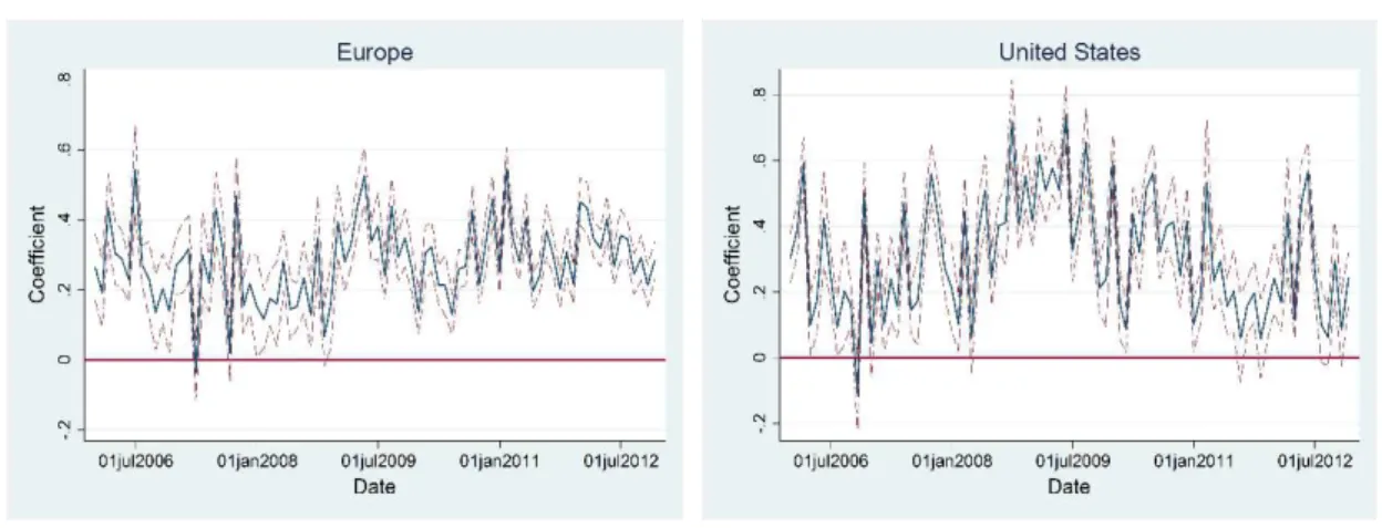
Figure A.2 in the appendix shows the coefficients estimates for both corporate (panel A) and
sovereign (panel B) bond funds, for the European and the US regions. Focusing on the top left panel,
Europe presents an average autocorrelation of 0.25 before the crisis period, value that increases to
more than 0.4 at the peak of the 2008 financial crisis. Since then, the average autocorrelation of the
European corporate funds decreased but to higher values than the ones that were verified before the
emergence of the crisis. Similarly, the US average autocorrelation of corporate bonds funds also
increased a lot at the end of 2008, achieving a value of 0.4. However, whereas European corporate
funds still face an autocorrelation much higher than the one before crisis, the US average
autocorrelation decreased to values similar to the ones before crisis.
About sovereign funds autocorrelation, before crisis both European and the US regions
presented an average autocorrelation of 0.3. However, during 2008, the average US sovereign funds
autocorrelation more than doubled its value before crisis, contrary to what happened with the
European corporate funds that had its increase slightly later and less pronounced. It is important to
notice that the behaviour of the after peak period autocorrelations in both regions is slightly different.
In the US there was a considerably decrease of the value of the autocorrelation at the beginning of
2011 that was extended until mid-2012, when there was a fast local peak. On the other side of the
but after that year the autocorrelation tended to increase. Therefore, based on the parametric, we
reject the null hypothesis that the past flow is unrelated to future flows.
Alternatively, a non-parametric methodology is performed. In this method, funds are considered
as Winners or Losers depending on their performance over consecutive periods. A fund is
considered as Winner (Loser) if its performance is above (below) the median performance. This
process was done twice, so that in the second time it would be possible to identify repeated winners
and losers. Thus, a Winner-Winner (WW) is a fund that was Winner in the previous period and still
is Winner in the current period. Loser-Loser (LL), Winner-Loser (WL) and Loser-Winner (LW)
follow the same idea of WW. Table A.5 in the appendix summarizes the frequency with which
winners and losers repeat, as well as the respective odds-ratio (OR) calculated through the following
formula for each year:
𝑂𝑅𝑡= 𝑊𝑊𝑊𝐿𝑡𝑡×𝐿𝑊×𝐿𝐿𝑡𝑡 (3)
As previously stated, under the null hypothesis the past flow performance in the previous year is
unrelated to the current flow performance. In that case, the odds-ratio equals one and the logarithm
of the odds-ratio follows a standard normal distribution:
ln (𝑂𝑅)
𝜎ln(𝑂𝑅)6~𝑁(0,1) (4)
For all years, we reject the null hypothesis at a 1% significance level that consequently means
that the winners of the previous year correspond to the winner of the current year. Therefore, we
reach the same conclusion both with the parametric and the non-parametric methods that bond fund
flows are strongly persistence especially during crises.
4.5.Control Variables
Focusing on table A.2 in the appendix, the main differences between both regions occur in the
size, cumulative flow, load and age of bond funds. The US funds presented on average higher total
net assets than European funds, which is visible through the size of funds ($4.37 and $4.06 million,
respectively) and the cumulative flows ($680.73 and $435.51 million, respectively). Another
important difference is related with the fund age that in the US tends to be larger than in Europe
(192.07 against 160.49 months, respectively). On the other hand, load tends to be larger in Europe
than in the US ($2.63 against $2.01), as well as the total expense ratio (0.93 for Europe and 0.90 for
the US).
Table A.6 shows the cross-sectional correlations of the control variables, for all sample (panel
A) and for the largest outflows (panel B), for the European region. Focusing on panel A, flow
standard deviation correlates positively with both lagged flow and total expense ratio (0.411 and
0.103 respectively), but negatively with size, age and benchmark (-0.317, -0.552 and -0.355,
respectively). As expected, size and cumulative flow have a positive correlation (0.694), as well as
load and total expensive ratio (0.475). Regarding panel B, the correlations among the control
variables are identical to the top panel ones, but now they tend to have lower values, as is the case
of correlation between size and cumulative flow (0.629). In what concerns to the sign of the
correlations, the main differences occur with correlations between benchmark and the other control
variables that now are more negatively than positively correlated.
Table A.7 provides the correlations among control variables for the US region. In panel A it is
shown the correlations for all sample. Similarly to what happen in the European region, size and
cumulative flow are highly correlated with each other (0.687). On the other side, cumulative flow
is negatively correlated with total expense ratio and flow standard deviation (-0.202 and -0.165,
respectively). As expected the latter is also negatively correlated with the size of funds (-0.315).
Concerning the bottom panel, the correlations among the variables tended to decrease, but in the
5. Methodology
So far the results are not enough to understand which variables can drive a fund run. Because of
that, in this section I will propose a model that might help us to achieve the main variables that
explain fund runs.
Funds can be seen as a game in real life. Independently of the type of game, when a game is
good and popular it tends to draw the attention of several players that will want to play more time
regardless the other players opinion.. However, when a game is not sufficiently good to draw
players’ attention it will lose its popularity and consequently its players and, at the end, nobody will
want to play that game. Financially speaking, whenever a fund has a good flow performance it tends
to attract more investors to put part of their effort into this fund. When the fund performance is good,
independently of its origin, investors have no fear to invest and do not take into account moves of
the other players. However, when the fund performance starts to decrease investors will tend to
deviate their investment from this bad fund starting a snow-ball effect, more specifically a fund run.
Due to all those specifications, the model needs to take into consideration both common and
specific fund shocks. For that, the model is based on three main conditional quantiles regressions -
10th, 50th and 90th– that will account for the two types of shocks and it will be developed around the
mean quantile and then it will diverge for the right and left tails. The advantage of using quantile
regression instead of panel OLS is that with the former the whole shape of the distribution is taken
into account rather than just the simple mean as it happens with the latter.
The following model was introduced by Koenker & Bassett (1978) and more recently used by
Schmidt et al. (2013). Let the dependent variable be 𝑌𝑖𝑡 and the independent conditioning variables
be the matrix 𝑋𝑖𝑡, in such way that:
𝑌𝑖𝑡 = 𝑓(𝑋𝑖𝑡, 𝛽) + 𝜀𝑖𝑡 (5)
and satisfies the econometric zero conditional mean assumption that 𝐸[𝜀𝑖𝑡|𝑋𝑖,𝑡] = 0, with the
interest and therefore whenever we change its value we are automatically changing the quantile of
interest. In order to account for all quantiles of interest, the following quantiles regressions
specifications were taken into consideration:
𝑌𝑖𝑡 = 𝑓0(𝑋𝑖𝑡, 𝛽) = 𝑋𝑖𝑡′𝛽0+ 𝜀𝑖𝑡0 𝑃[𝜀𝑖𝑡0 < 0|𝑋𝑖𝑡] = 0.5
𝑌𝑖𝑡 = 𝑓1(𝑋𝑖𝑡, 𝛽) = 𝑋𝑖𝑡′𝛽0− exp [𝑋𝑖𝑡′𝛽1] + 𝜀𝑖𝑡1 𝑃[𝜀𝑖𝑡1 < 0|𝑋𝑖𝑡] = 0.1
𝑌𝑖𝑡 = 𝑓2(𝑋𝑖𝑡, 𝛽) = 𝑋𝑖𝑡′𝛽0+ exp [𝑋𝑖𝑡′𝛽2] + 𝜀𝑖𝑡2 𝑃[𝜀𝑖𝑡2 < 0|𝑋𝑖𝑡] = 0.9
(6)
The different betas captures different shocks. 𝛽0 is responsible for the common shock that affects
all funds, whereas 𝛽1 and 𝛽2 capture the additional effect of shocks that affect the left and right tails,
respectively, of the distribution.
The stated model can be written in a different way, using positive random variables with
𝑃[𝜂𝑖𝑡< 1|𝑋𝑖𝑡] = 0.8 and a Bernoulli random variable (𝐷𝑖𝑡) that equals one with a probability of 0.57:
𝑌𝑖𝑡 = 𝑋𝑖𝑡′𝛽0− 𝐷𝑖𝑡exp[𝑋𝑖𝑡′𝛽1] 𝜂𝑖𝑡+ (1 − 𝐷𝑖𝑡)exp [𝑋𝑖𝑡′𝛽2]𝜂𝑖𝑡 (7) The parameters were then estimated following the process stated in Schmidt (2012). The
estimation of 𝛽0 was based on linear quantile regression and only after this estimation had been
made it was possible to proceed with the estimation of both 𝛽1 and 𝛽2 by dividing the sample
according to the sign of the residuals (positive for 𝛽1 and negative for 𝛽2) and doing additional
linear quantile regression on the logarithm of the same residuals8. 𝛽0 was then replaced by the
estimated one, 𝛽̂0, in the median quantile regression. The same was done for both left and right tails,
but with a slight difference at the time of estimating the respective standard errors. For both 𝛽1 and
𝛽2, the respective standard errors were estimated through bootstrapping, since the theoretical
distribution of the sub-sample was unknown. The bootstrap algorithm drew many independent
bootstrap samples through replication and then estimated both 𝛽1 and 𝛽2 standard errors.
7 To understand why the probability equals 0.5, notice that if 𝑃(𝜂
𝑖𝑡< 1|𝑋𝑖𝑡) = 0.8, then 𝑃(𝑌𝑖𝑡< 𝑋𝑖𝑡′𝛽0− exp[𝑋𝑖𝑡′𝛽1]| 𝑋𝑖𝑡) =
𝑃(𝐷𝑖𝑡= 1|𝑋𝑖𝑡) × 𝑃(𝜂𝑖𝑡> 1|𝑋𝑖𝑡) = 0.5 × (1 − 0.8) = 0.1
8 Notice that 𝜀
𝑖𝑡= 𝑌𝑖𝑡− 𝑋𝑖𝑡′𝛽0 and if 𝑌𝑖𝑡− 𝑋𝑖𝑡′𝛽0> 0 then 𝑌𝑖𝑡− 𝑋𝑖𝑡𝛽0= exp[𝑋𝑖𝑡′𝛽2] 𝜂𝑖𝑡. Taking the logs we get log[𝑌𝑖𝑡− 𝑋𝑖𝑡′𝛽0] =
𝑋𝑖𝑡′𝛽2+ 𝑙𝑜𝑔𝜂𝑖𝑡. Because it was assumed that 𝑃(𝜂𝑖𝑡< 1|𝑋𝑖𝑡) = 𝑃(𝑙𝑜𝑔 𝜂𝑖𝑡< 0|𝑋𝑖𝑡) = 0.8, the transformed model imposes that 𝛼 =
6. Empirical results
The stated model helps us to better understand which funds are more vulnerable to a possible
run. In order to figure out both common and specific shocks, the whole sample is firstly evaluated
and then divided in three sub-samples that are evaluated individually. The first sub-sample includes
monthly observations from year 2002 to 2006 (thereafter: “Before Crisis”), the second from year
2007 to 2011 (“Crisis Period”) and the last sub-sample is only composed by year 2012 (“After
Crisis”) due to the lack of observations after that year. The analysis is repeated for the European and
the US regions, taking into consideration both corporate and sovereign funds. For all cases, the
dependent variable is the monthly fund flow, calculated as the percentage of lagged Total Net
Assets. In the following two tables (2 and 3), there are represented the common shock estimated
coefficients (“Common Shock”) that in the last section are represented by β0, as well as the left and
right tails estimated coefficients (“Left Tail” and “Right Tail”), respectively denominated by β1 and
β2 in the last section.
6.1. Corporate funds
6.1.1. All sample
Table 2 provides the estimated coefficients of the quantile regression from equation (6) for
corporate funds geographically focused on the US and Europe. From the observation of panel A, it
is possible to conclude that the main explanatory variables predict fund flow. The exception is the
institutional class that is only statistically significant for the right tail, representing the funds with
largest inflows (lowest outflows), meaning that funds owned by institutional investors had lower
inflows than retailed ones. Returns have an important statistical significance, since they are the
estimator that has the highest coefficient across all shocks, stating that high return in left tail funds
tend to have larger outflows. Moreover, regarding the flow standard deviation, although it is always
statistically significant, its coefficient increases a lot when we consider left and right tails, reflecting
fund flows prediction, which means that older funds with high returns tend to have largest outflows
in the left tail. Contrarily to what happens with the US, in Europe (panel B) all control variables are
statistically significant to predict funds flow. Here, returns have a negative impact in flow prediction
in the left tail, having coefficients much lower than in the US case. Flow standard deviation also
presents a great coefficient variation when we consider either left or right tails compared to what
happens in the common shock. In this case, older funds owned by institutional investors tend to
have lower inflows than the ones owned by retail investors in the right tail.
6.1.2. Before Crisis
Through the observation of column “Before Crisis” of panel A it is possible to conclude that
funds with high returns have more outflows in the left tail of the distribution, contrarily to what
happens with funds with higher returns where, on the right tail, they tend to have the largest inflows.
Moreover, funds with higher TER contribute to lower outflows in the left tail and lower inflows in
the right tail. Regarding panel B, most of the variables are significant to flow prediction. On average,
funds which are owned by institutional investors, tend to have larger outflows in the left tail than in
the right tail. In what concerns to the flow standard deviation, it is very strong in both tails, indicating
high flow persistence. About the TER, the right tail has lower inflows.
6.1.3. Crisis Period
Panel A tells us that, once again, that larger return funds tend to have the largest outflows in the
left tail and larger inflows in the right tail of the distribution. About age, it also has a negative impact
in both left and right tails. During this period most investors tend to choose the right tail of the
distribution, contrarily to what happened in the period before, where TER coefficient was much
higher in the left tail. In the European case (panel B), funds with higher returns tend to face larger
outflows in the left tail, contrarily to what happens in the right tail, where high return funds tend to
median. Those results are in agreement with panel A of figure A.1 in the appendix which shows
that in the US investors tend to choose the right tail but in Europe they tend to invest in the left tail.
6.1.4. After Crisis
Focusing now on the “After Crisis” column, in the US, older funds with high returns tend to
have lower outflows in the left tail, contrarily to what happens in Europe, where older funds with
higher returns tend to have larger outflows. It is important to note that in this period, the effect of the
coefficients decreases compared to the crisis period.
Table 2 – Fund Flow Panel Regressions: Corporate bond funds
Panel A: United States Panel B: Europe Note:
The numbers inside brackets represents the t-values.
*, ** and *** indicate significance at the 10%, 5% and 1% level, respectively. Variable Common Shock
All sample Before Crisis Crisis Period After Crisis
Return 0.14794*** 0.20007*** 0.1336*** 0.1454***
[37.2] [22.8] [28.2] [7.5]
TER -0.00076*** -0.17567*** -0.00055*** 0.00219***
[-4.1] [-5.9] [-2.1] [3.4]
FlowS..D. 0.04629*** 0.04528*** 0.04589*** 0.04955***
[26.2] [14.7] [18.5] [8.6]
Age -0.00001*** -0.00001*** -0.00001*** -0.00001***
[-15.5] [-9.5] [-10.0] [-4.6]
Inst. Class 0.00021 -0.00052 0.00069* 0.00175*
[0.8] [-1.3] [1.7] [1.7]
Variable Left Tail
All sample Before Crisis Crisis Period After Crisis
Return -4.33449*** -6.80262*** -3.90074*** 1.47043
[-10.6] [-10.9] [-7.9] [1.1]
TER 0.07036*** 0.14438*** 0.03061 -0.21623**
[4.4] [5.6] [1.2] [-2.5]
FlowS..D. 8.07815*** 9.15864*** 7.78503*** 7.48785***
[42.4] [27.8] [30.3] [21.6]
Age -0.00098*** -0.00124*** -0.00087*** 0.00002
[-11.3] [-8.1] [-6.7] [0.1]
Inst. Class 0.02856 0.05702 0.00798 -0.03570
[1.4] [1.1] [0.2] [-0.7]
Variable Right Tail
All sample Before Crisis Crisis Period After Crisis
Return 4.5153*** 5.02828*** 4.43703*** 2.9107*
[10.0] [6.2] [9.5] [1.9]
TER 0.01318 -0.04498* 0.07717** 0.02679
[0.8] [-1.8] [2.4] [0.5]
FlowS..D. 11.8211*** 13.4069*** 11.7718*** 9.1782***
[62.8] [43.6] [39.5] [22.7]
Age -0.00122*** -0.00105*** -0.00134*** -0.00095***
[-15.1] [-8.7] [-9.5] [-5.7]
Inst. Class -0.14418*** -0.20761*** -0.11660*** 0.09017
[-5.2] [-4.3] [-3.0] [0.8]
Variable Common Shock
All sample Before Crisis Crisis Period After Crisis
Return 0.01497*** -0.0095*** 0.0201364*** 0.01617***
[9.3] [-2.5] [8.8] [3.3]
TER -0.00397*** -0.00541*** -0.00468*** -0.00170***
[-29.5] [-20.7] [-20.9] [-4.9]
FlowS..D. 0.00239** 0.01779*** -0.00879*** 0.00462*
[2.1] [7.6] [-4.6] [1.8]
Age -0.00002*** -0.00003*** -0.00003*** -0.00001***
[-36.0] [-20.9] [-26.9] [-8.3]
Inst. Class 0.00058*** -0.00149*** 0.00128*** 0.00273***
[3.4] [-4.1] [4.8] [6.3]
Variable Left Tail
All sample Before Crisis Crisis Period After Crisis
Return -1.38841*** 0.71650 -1.78379*** -1.32812*
[-8.7] [1.5] [-8.1] [-1.9]
TER 0.02721 0.07617*** -0.00473 -0.09445
[1.6] [2.8] [-0.2] [-1.2]
FlowS..D. 10.849*** 10.131*** 11.79*** 7.2916***
[51.9] [38.8] [76.5] [10.8]
Age 0.00030*** -0.00045*** 0.00077*** -0.00082***
[2.9] [-2.6] [6.1] [-3.2]
Inst. Class 0.06785*** -0.22457*** 0.19930*** 0.11603*
[2.8] [-4.7] [4.9] [1.9]
Variable Right Tail
All sample Before Crisis Crisis Period After Crisis
Return 0.76939*** 0.46705 1.0031*** 1.9246**
[3.3] [1.1] [3.4] [2.2]
TER -0.10645*** -0.24612*** -0.05084 -0.04559
[-5.4] [-7.2] [-1.4] [-0.6]
FlowS..D. 14.3515*** 15.1533*** 14.5904*** 11.7074***
[62.2] [40.2] [76.4] [19.7]
Age -0.00069*** -0.00123*** -0.00029*** -0.0011***
[-6.1] [-9.9] [-3.1] [-5.0]
Inst. Class -0.19162*** -0.18663*** -0.18913*** -0.1943***
6.2. Sovereign funds
6.2.1. All sample
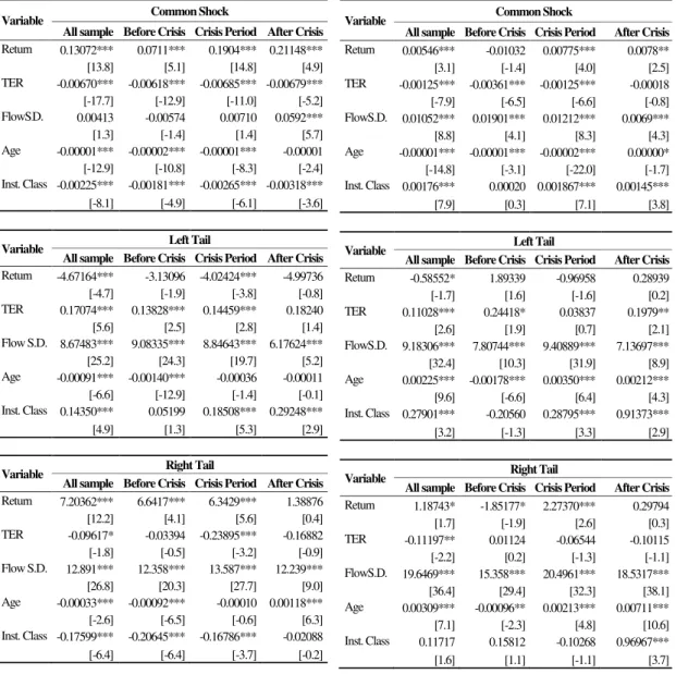
Table 3 presents the results of the estimated quantile regression of equation (6) for sovereign
funds geographically focused on the US and Europe. In most of the cases of panel A, all the
variables are statistically important to predict sovereign funds flow. The only exception is for the
flow standard deviation in the common shock. Once again, age has a negative impact for all shocks,
as well as the fund return in the left tail, meaning that older funds with high returns face higher
outflows. However, in the right tail, higher funds return tend to have large inflows if owned by retail
investors. Regarding European sovereign funds (panel B), flow standard deviation presents the
highest coefficient in both tails, indicating, for the right tail case, the tendency for capital to enter the
fund. In the common shock, age and TER have a negative impact on the flow prediction, situation
that is not verified in the left tail, where only return coefficient is negative, meaning that funds with
higher returns tended to have the largest outflows in the left tail. Similarly to what happens in the
US, institutional investors tend to have larger out/inflows than retail investors in all shocks in the
left/right tail.
6.2.2. Before Crisis
In this period, for both regions, TER coefficient is much higher in the left than in the right tail
(0.138 against -0.034, respectively, for the US and 0.244 against 0.011, for Europe). Regarding
funds’ age coefficient in both regions, the coefficients are very small and negative for both left and
right tails, which means that its contribution to funds’ flow prediction has a small impact.
6.2.3. Crisis Period
By the peak of the crisis, in the US, higher return funds have larger outflows than in Europe for
the respective left tail of the distribution. Regarding the flow standard deviation, in both regions, it
strongly predicts cross-sectional differences in outflows in both left and right tails. In addition, in
This fact is more pronounced in the US funds than in the European ones, contrary to what happens
in the left tail, which is in agreement with panel B of figure A.1.
6.2.4. After Crisis
After the considered period of crisis, flow standard deviation continues to strongly predict
outflows in both tails, contrary to what happens with age in both regions. Regarding TER, that is
close to the scale of investment, in both regions, the large-scale funds tend to have larger inflows in
the right tail of the distribution. Institutional class is again an important variable for funds flow
prediction in both regions, with institutional investors having less outflows than the retail ones in
the left tail of the distribution.
Table 3 – Fund Flow Panel Regressions: Sovereign bond funds
Panel A: United States Panel B: Europe
Variable Common Shock
All sample Before Crisis Crisis Period After Crisis
Return 0.13072*** 0.0711*** 0.1904*** 0.21148***
[13.8] [5.1] [14.8] [4.9]
TER -0.00670*** -0.00618*** -0.00685*** -0.00679***
[-17.7] [-12.9] [-11.0] [-5.2]
FlowS.D. 0.00413 -0.00574 0.00710 0.0592***
[1.3] [-1.4] [1.4] [5.7]
Age -0.00001*** -0.00002*** -0.00001*** -0.00001
[-12.9] [-10.8] [-8.3] [-2.4]
Inst. Class -0.00225*** -0.00181*** -0.00265*** -0.00318***
[-8.1] [-4.9] [-6.1] [-3.6]
Variable Left Tail
All sample Before Crisis Crisis Period After Crisis
Return -4.67164*** -3.13096 -4.02424*** -4.99736
[-4.7] [-1.9] [-3.8] [-0.8]
TER 0.17074*** 0.13828*** 0.14459*** 0.18240
[5.6] [2.5] [2.8] [1.4]
Flow S.D. 8.67483*** 9.08335*** 8.84643*** 6.17624***
[25.2] [24.3] [19.7] [5.2]
Age -0.00091*** -0.00140*** -0.00036 -0.00011
[-6.6] [-12.9] [-1.4] [-0.1]
Inst. Class 0.14350*** 0.05199 0.18508*** 0.29248***
[4.9] [1.3] [5.3] [2.9]
Variable Right Tail
All sample Before Crisis Crisis Period After Crisis
Return 7.20362*** 6.6417*** 6.3429*** 1.38876
[12.2] [4.1] [5.6] [0.4]
TER -0.09617* -0.03394 -0.23895*** -0.16882
[-1.8] [-0.5] [-3.2] [-0.9]
Flow S.D. 12.891*** 12.358*** 13.587*** 12.239***
[26.8] [20.3] [27.7] [9.0]
Age -0.00033*** -0.00092*** -0.00010 0.00118***
[-2.6] [-6.5] [-0.6] [6.3]
Inst. Class -0.17599*** -0.20645*** -0.16786*** -0.02088
[-6.4] [-6.4] [-3.7] [-0.2]
Variable Common Shock
All sample Before Crisis Crisis Period After Crisis
Return 0.00546*** -0.01032 0.00775*** 0.0078**
[3.1] [-1.4] [4.0] [2.5]
TER -0.00125*** -0.00361*** -0.00125*** -0.00018
[-7.9] [-6.5] [-6.6] [-0.8]
FlowS.D. 0.01052*** 0.01901*** 0.01212*** 0.0069***
[8.8] [4.1] [8.3] [4.3]
Age -0.00001*** -0.00001*** -0.00002*** 0.00000*
[-14.8] [-3.1] [-22.0] [-1.7]
Inst. Class 0.00176*** 0.00020 0.001867*** 0.00145***
[7.9] [0.3] [7.1] [3.8]
Variable Left Tail
All sample Before Crisis Crisis Period After Crisis
Return -0.58552* 1.89339 -0.96958 0.28939
[-1.7] [1.6] [-1.6] [0.2]
TER 0.11028*** 0.24418* 0.03837 0.1979**
[2.6] [1.9] [0.7] [2.1]
FlowS.D. 9.18306*** 7.80744*** 9.40889*** 7.13697***
[32.4] [10.3] [31.9] [8.9]
Age 0.00225*** -0.00178*** 0.00350*** 0.00212***
[9.6] [-6.6] [6.4] [4.3]
Inst. Class 0.27901*** -0.20560 0.28795*** 0.91373***
[3.2] [-1.3] [3.3] [2.9]
Variable Right Tail
All sample Before Crisis Crisis Period After Crisis
Return 1.18743* -1.85177* 2.27370*** 0.29794
[1.7] [-1.9] [2.6] [0.3]
TER -0.11197** 0.01124 -0.06544 -0.10115
[-2.2] [0.2] [-1.3] [-1.1]
FlowS.D. 19.6469*** 15.358*** 20.4961*** 18.5317***
[36.4] [29.4] [32.3] [38.1]
Age 0.00309*** -0.00096** 0.00213*** 0.00711***
[7.1] [-2.3] [4.8] [10.6]
Inst. Class 0.11717 0.15812 -0.10268 0.96967***
7. Conclusion
As time goes by, bond funds have been gaining importance in the finance of economies, but
there is still a lot of work to do to better understand runs of those types of funds. With this thesis I
provide an empirical analysis of runs on bond funds during the period between 2002 and 2012 and
its original contribution lies in identifying which funds, in terms of their characteristics, are more
likely to suffer a run.
I find that cross-sectional correlations tend to have a similar impact on both US’ and European
funds, although in the case of the bond issuer entity, it influences more the US’ funds than the
European ones. Regarding the European case, countries with lower credit rating tend to have, on
average, more outflows than countries with higher credit ratings, especially with sovereign funds,
which indicates that higher risk level countries tend to face more funds runs.
Based on the panel quantile regressions, during the financial crisis period runs are more
pronounced than in the remaining periods. Regarding the characteristics of funds, higher fund return
tend to have larger outflows and inflows in the left and right tails, respectively, until the crisis period
for corporate funds. After crisis, those older corporate funds with higher returns tend to have lower
outflows in the left tail in the US, but larger outflows in the same tail for Europe, which indicates
that most of the corporate geographically focused on Europe are still facing significant outflows.
Regarding sovereign funds, before crisis, in the US, funds higher TER and owned by institutional
investors tend to have low outflows in the left tail, similarly to what happens in Europe in the right
tail. During the crisis period, in both regions, funds with higher returns and owned by institutional
investors face larger outflows both in the left and right tails. After crisis, large-scale funds have large
outflows in the right tail, with institutional investors having lower outflows in the left tail.
To sum up, for the European case, runs continued to be pronounced after the peak crisis period,
situation that is not as visible for the US case. Those results are consistent with most of the recent
References
Brown, Stephen, Goetzmann, William, Ibbotson, Roger and Ross, Stephen. 1992.
“Survivorship Bias in Performance Studies”. The Review of Financial Studies, 5(4): 553-580.
Chen Qi, Itay Goldstein and Wei Jiang. 2010. “Payoff complementaries and financial fragility:
Evidence from mutual fund outflows”. The Journal of Financial Economics, 97: 239-262.
Diamond, Douglas W. and Philip H. Dybvig. 1983. “Bank Runs, Deposit Insurance, and
Liquidity”. TheJournal of Political Economy, 91(3): 401-419.
Gorton, Gary and Pennacchi, George. 1993. “Money market funds and finance companies: Are
They the Banks of the Future?”, Strutural Change in Banking.
Jacklin, C.J. and S. Bhattacharya. 1988. “Distinguishing panics and information-based bank runs:
Welfare and policy implications”. The Journal of Political Economy, 96: 568-592.
Jank, Stepahn and Michael Wedow. 2010. “Sturm und Drang in Money Market Funds: When
Money Market Funds Cease to Be Narrow”. Working Paper, University of Cologne and ECB.
Pennacchi, George.2012. “Narrow Banking”. Annual Review of Financial Economics, 4.
Schmidt, Lawrence. 2012. “Quantile Spacings: A Simple Method for the Joint Estimation of
Multiple Quantiles”. Working Paper, UCSD.
Wermers, Russ, Lawrence Schmidt and Allan Timmermann. 2013. “Runs on Money Market
Appendices
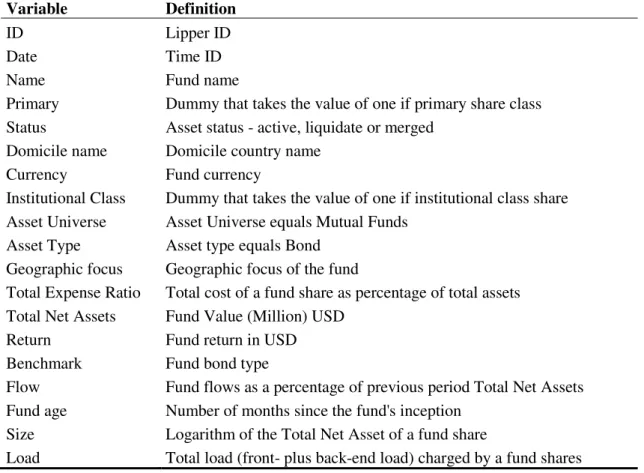
Table A.1 – Definition of the variables
This table presents the definition of the variables used in this study. All variables were obtained from Lipper database.
Variable Definition
ID Lipper ID
Date Time ID
Name Fund name
Primary Dummy that takes the value of one if primary share class Status Asset status - active, liquidate or merged
Domicile name Domicile country name
Currency Fund currency
Institutional Class Dummy that takes the value of one if institutional class share Asset Universe Asset Universe equals Mutual Funds
Asset Type Asset type equals Bond Geographic focus Geographic focus of the fund
Total Expense Ratio Total cost of a fund share as percentage of total assets Total Net Assets Fund Value (Million) USD
Return Fund return in USD
Benchmark Fund bond type
Flow Fund flows as a percentage of previous period Total Net Assets Fund age Number of months since the fund's inception
Size Logarithm of the Total Net Asset of a fund share
Table A.2 – Descriptive statistics of the control variables
This table presents the descriptive statistics of the cross-sectional bond funds for Europe (Panel
A) and the US (Panel B) regions between 2002 and 2012. LagFlow is the lagged fund flow as a
percentage of lagged Total Net Assets, TER represents the total expense ratio of the fund, Flow
S.D. is the standard deviation of monthly percentages changes in funds’ assets, Size stands for the
logarithm of the Total Net Asset of a fund share, Cflow represents the cumulative flow, Load is
the total load (front- plus back-end load) charged by a fund shares, Age stands for the fund age
calculated since its inception and LagReturn is the lagged fund return.
Panel A: European bond funds
Variable Mean S.D. Min Quantiles Max
0.25 Mdn 0.75
LagFlow 0.00 0.10 -0.35 -0.02 0.00 0.01 0.62
TER 0.93 0.43 0.04 0.61 0.93 1.19 2.38
Flow S.D. 0.08 0.05 0.00 0.04 0.07 0.11 0.56
Size 4.06 1.82 -2.53 2.97 4.16 5.29 8.16
Cflow 435.51 911.70 0.16 39.68 129.11 401.57 7010.80
Load 2.63 2.31 0.00 0.30 2.50 4.00 11.50
Age 160.49 97.05 0.00 92.37 152.20 217.10 600.67
LagReturn 0.01 0.03 -0.09 -0.01 0.01 0.03 0.09
Panel B: US bond funds
Variable Mean S.D. Min Quantiles Max
0.25 Mdn 0.75
LagFlow 0.01 0.10 -0.35 -0.02 0.00 0.01 0.62
TER 0.90 0.44 0.04 0.61 0.83 1.08 2.38
Flow S.D. 0.08 0.06 0.00 0.03 0.07 0.11 0.49 Size 4.37 1.97 -2.53 3.21 4.49 5.72 8.16 Cflow 680.73 1330.11 0.16 50.80 180.20 612.40 7010.80 Load 2.01 2.61 0.00 0.00 0.10 4.00 11.50
Age 192.07 120.61 0.93 99.43 186.70 267.87 1362.57
Table A.3 – Yearly Number of Total Net Assets (TNA)
The table presents the TNA of the funds across European countries and the US until the end of 2012. TNA is
defined as the sum of all total fund value (in $ million). All the values presented below are in $ thousand
million.
Country 2002 2003 2004 2005 2006 2007 2008 2009 2010 2011 2012 N
Austria 0.158 54.00 77.61 81.68 81.08 74.72 70.50 66.94 62.77 59.58 55.82 6.27
Belgium 5.533 23.71 24.03 19.21 17.29 14.03 14.10 17.38 15.55 13.43 6.902 2.00
Czech Republic 11.79 23.34 28.66 33.74 41.68 47.30 47.86 32.96 35.82 34.17 28.95 3.14
Denmark 2.846 10.83 15.80 18.70 15.92 28.53 43.80 47.92 49.77 74.34 91.86 3.90
Estonia - - - 0.221 0.941 0.674 0.148 - - 0.03
Finland - 0.499 0.460 0.181 0.157 0.023 - - - 0.06
France 1.823 35.85 67.11 75.99 59.79 46.95 44.13 33.23 28.29 26.24 21.18 5.86
Germany 13.38 166.0 247.4 234.5 219.6 181.2 158.6 146.0 147.9 149.6 144.2 8.21
Greece 5.808 9.048 10.64 10.37 5.801 0.844 0.829 0.922 3.135 3.262 1.495 0.90
Hungary 0.586 1.423 0.809 1.194 1.920 25.53 18.42 11.87 19.27 19.34 14.10 3.06
Italy 0.419 34.31 49.85 41.95 54.44 38.61 22.58 25.51 16.75 19.07 25.47 1.07
Lithuania - - 0.010 0.003 0.013 0.054 0.136 0.026 0.046 0.000 - 0.08
Netherlands 0.209 1.329 1.168 3.876 6.354 6.272 6.757 6.183 6.101 5.398 4.764 0.94
Norway 0.548 1.914 5.189 9.771 14.59 0.606 26.96 27.40 43.21 0.978 84.88 1.74
Poland 19.44 38.09 24.01 35.38 32.39 30.61 34.24 32.50 45.88 49.26 58.42 3.94
Portugal 7.450 10.66 20.22 23.11 18.36 11.22 9.086 7.058 9.291 10.64 10.78 0.90
Romania - - - 0.210 0.739 2.460 3.155 3.024 0.06
Slovakia - 0.145 1.250 2.464 2.895 2.720 3.041 2.585 2.626 2.418 1.903 0.61
Spain 19.73 56.58 76.23 82.53 72.28 57.61 51.76 3.382 77.43 214.4 241.1 15.0
Sweden 4.337 37.98 60.53 70.77 80.31 92.87 118.7 115.1 136.2 160.2 174.5 3.84
Switzerland 1.802 157.7 248.7 292.5 379.4 446.1 446.0 420.7 461.9 538.6 533.0 16.2
United Kingdom 26.04 518.5 765.0 931.7 1,177 1,370 1,219 1,098 1,154 1,210 1,286 37.6
Europe 596.6 5,113 7,228 7,955 8,228 8,436 7,327 6,496 6,881 7,036 6,752 398
Table A.4 – Descriptive statistics of funds flows as of December 2012
This table shows the descriptive statistics of funds flows as of December 2012. Specifically, the
mean, standard deviation and a range of quantiles during the sample period is presented for each
European country and for the US.
Country N Mean S.D. Min Quantiles Max
0.25 Mdn 0.75
Austria 3,705 0.00 0.06 -0.35 -0.01 0.00 0.00 0.62
Belgium 1,531 -0.01 0.09 -0.35 -0.02 0.00 0.00 0.62
Czech Republic 2,330 0.00 0.08 -0.35 -0.01 0.00 0.00 0.62
Denmark 2,854 0.01 0.10 -0.35 -0.02 0.00 0.01 0.62
Estonia 33 0.02 0.08 -0.16 0.00 0.00 0.00 0.33
Finland 45 -0.05 0.08 -0.35 -0.05 -0.02 -0.01 0.09
France 5,175 -0.01 0.06 -0.35 -0.02 -0.01 0.00 0.62
Germany 6,961 -0.01 0.07 -0.35 -0.02 -0.01 0.00 0.62
Greece 470 -0.01 0.09 -0.35 -0.02 -0.01 0.00 0.62
Hungary 1,990 0.00 0.10 -0.35 -0.03 -0.01 0.02 0.62
Italy 930 0.01 0.14 -0.35 -0.03 -0.01 0.01 0.62
Lithuania 56 0.04 0.23 -0.35 -0.06 0.00 0.11 0.62
Netherlands 369 -0.02 0.05 -0.33 -0.03 -0.01 0.00 0.17
Norway 1,444 0.02 0.11 -0.35 -0.01 0.00 0.04 0.62
Poland 3,273 0.03 0.15 -0.35 -0.04 0.00 0.05 0.62
Portugal 769 -0.01 0.07 -0.35 -0.02 0.00 0.00 0.62
Romania 58 0.05 0.13 0.00 0.00 0.00 0.03 0.62
Slovakia 499 0.00 0.09 -0.35 -0.02 0.00 0.01 0.62
Spain 13,469 0.00 0.09 -0.35 -0.02 0.00 0.00 0.62
Sweden 2,927 0.01 0.09 -0.35 -0.02 0.00 0.02 0.62
Switzerland 14,409 0.00 0.08 -0.35 -0.01 0.00 0.01 0.62 United Kingdom 30,369 0.01 0.09 -0.35 -0.01 0.00 0.01 0.62
Europe 319,182 0.00 0.10 -0.35 -0.02 0.00 0.01 0.62
Figure A.1 – Quantiles of monthly flows
This figure shows the quantiles of monthly flows for Europe and the US. In Panel A it is shown
the quantiles for corporate funds for both regions, whereas in Panel B it is represented the
quantiles for sovereign funds.
Panel A: Corporate Funds
Figure A.2 – AR(1) coefficients
This figure shows the AR(1) coefficients estimates for both corporate (Panel A) and sovereign
(Panel B) bond funds, for the European and the US regions.
Panel A – AR(1) coefficients estimates for Corporate funds
Panel B – AR(1) coefficients estimates for sovereign funds
Table A.5 – Performance Persistence of Bond Funds: Repeated Winners and Losers
Funds were classified into winners (annual flow above media) and losers (annual flow below
median) for each year between 2002 and 2012. Winner-Winner (WW) shows the number of funds
that were winners in the previous period and still are Winner in the current period. Winner-Loser
(WL) indicates the number of funds that were winners in the previous period but are not in the
current period. The null hypothesis, past flow performance in the previous year is unrelated to the
Year Total Winner- Winner- Loser- Loser- Odds- z Winner Loser Winner Loser ratio
2002 5,132 1,526 368 2,302 936 1.7 7.5
2003 5,279 1,136 1,139 1,116 1,888 1.7 9.3
2004 5,320 1,155 1,176 1,001 1,988 2.0 11.8
2005 5,378 1,136 865 1,402 1,975 1.9 10.8
2006 5,340 1,264 990 1,363 1,723 1.6 8.6
2007 5,260 1,315 866 1,606 1,473 1.4 5.8
2008 5,236 1,045 1,253 952 1,986 1.7 9.6
2009 5,599 1,000 1,382 888 2,329 1.9 11.2
2010 6,009 1,274 1,243 1,427 2,065 1.5 7.5
2011 6,454 1,185 1,574 1,080 2,615 1.8 11.4
2012 6,938 1,316 1,666 1,154 2,802 1.9 12.8
Table A.6 – Cross-sectional correlations of the control variables for Europe
This table presents the cross-sectional correlations of the control variables for Europe. The top
panel shows the correlations for all sample, whereas the bottom panel presents the same
correlations but for the funds that had the largest outflows between 2002 and 2012.
Panel A: All sample correlations
Correlation LagFlow TER Flow S.D. Size Cflow Load Age LagReturn Benchmark
LagFlow 1.000
TER -0.013 1.000
Flow S.D. 0.105 -0.009 1.000 Size 0.013 -0.184 -0.204 1.000 Cflow -0.010 -0.070 -0.111 0.643 1.000 Load 0.011 0.132 0.028 0.008 -0.022 1.000
Age -0.058 0.035 -0.287 0.214 0.148 -0.165 1.000
LagReturn 0.030 0.001 -0.002 0.015 0.009 -0.002 0.008 1.000 Benchmark 0.012 -0.016 0.039 -0.052 -0.063 0.149 -0.149 -0.007 1.000
Panel B: Correlations of the bottom tercile
Correlation LagFlow TER Flow S.D. Size Cflow Load Age LagReturn Benchmark
LagFlow 1.000
TER 0.034 1.000
Flow S.D. 0.371 0.025 1.000
Size -0.089 -0.176 -0.239 1.000
Cflow -0.069 -0.059 -0.136 0.629 1.000 Load 0.009 0.174 0.047 0.007 -0.003 1.000
Age -0.105 0.022 -0.303 0.227 0.153 -0.121 1.000
Table A.7 – Cross-sectional correlations of the control variables for the US
This table presents the cross-sectional correlations of the control variables for the US. The top
panel shows the correlations for all sample, whereas the bottom panel presents the same
correlations but for the funds that had the largest outflows between 2002 and 2012.
Panel A: All sample correlations
Correlation LagFlow TER Flow S.D. Size Cflow Load Age LagReturn Benchmark
LagFlow 1.000
TER -0.010 1.000
Flow S.D. 0.140 0.069 1.000
Size 0.010 -0.312 -0.315 1.000
Cflow 0.000 -0.202 -0.165 0.687 1.000 Load 0.021 0.372 -0.042 -0.036 -0.047 1.000 Age -0.090 -0.066 -0.542 0.371 0.274 0.038 1.000 LagReturn 0.048 0.021 0.001 0.028 0.021 0.022 -0.001 1.000
Benchmark -0.033 -0.291 -0.378 0.089 0.010 -0.103 0.278 -0.030 1.000
Panel B: Correlations of the bottom tercile
Correlation LagFlow TER Flow S.D. Size Cflow Load Age LagReturn Benchmark
LagFlow 1.000
TER 0.075 1.000
Flow S.D. 0.411 0.103 1.000 Size -0.169 -0.280 -0.317 1.000 Cflow -0.104 -0.178 -0.182 0.694 1.000 Load 0.021 0.475 -0.004 -0.099 -0.083 1.000
Age -0.216 -0.097 -0.552 0.354 0.284 -0.006 1.000
LagReturn 0.031 0.024 0.006 0.037 0.025 0.015 -0.006 1.000