Correlation Between the Mechanical Cycling Behavior and Microstructure in Laser Welded Joints Using NiTi Memory Shape Alloys

(1)

João Pedro de Sousa Oliveira

Licenciado em Engenharia de Materiais

Correlation Between the Mechanical

Cycling Behavior and Microstructure in

Laser Welded Joints Using NiTi Memory

Shape Alloys

Dissertação para obtenção do Grau de Mestre em Engenharia de Materiais

Orientador: Doutor Francisco Manuel Braz Fernandes,

Professor Associado com Agregação, Faculdade de

Ciências e Tecnologia da Universidade Nova de Lisboa

Co-orientador: Doutora Rosa Maria Mendes Miranda,

Professora Associada com Agregação, Faculdade de

Ciências e Tecnologia da Universidade Nova de Lisboa

Júri:

Presidente: Prof. Doutor Rui Jorge Cordeiro Silva

Arguente: Prof. Doutora Maria Luísa Coutinho Gomes de Almeida Vogais: Prof. Doutor Francisco Manuel Braz Fernandes

(2)

(3)

Correlation Between the Mechanical Cycling Behavior and Microstructure in Laser Welded Joints Using NiTi Memory Shape Alloys

(4)

(5)

i

Agradecimentos

Este trabalho não poderia ter sido realizado sem a ajuda e colaboração dos meus orientadores: Professor Doutor Braz Fernandes e Professora Doutora Rosa Miranda. O seu apoio foi fundamental para a realização deste trabalho e tenho de agradecer por toda a ajuda que me prestaram, disponibilidade total para esclarecer as dúvidas que foram surgindo ao longo deste trabalho e pela sua amizade.

Gostaria de agradecer ao financiamento da FCT/MCTES para o projecto ‘Joining micro to small scale systems in shape memory alloys using last generation infrared lasers’ (PTDC/EME-TME/100990/2008).

Agradeço o apoio de DESY para o tempo de feixe I-20100250 EC na linha P-07 (HEMS, PETRA-III).

Quero também agradecer à Joana Duarte pela companhia que me foi fazendo e amizade que me deu durante estes anos. Não posso deixar de recordar os meus colegas que me foram acompanhando ao longo destes anos: Ruben Raposo, Salomé Moço, Andreia Alexandrino, Sara Gil e todos os outros que aqui não refiro. Ao Dr. Mahesh um agradecimento pela ajuda que foi dando ao longo desta tese.

Aos meus pais, por todo o seu apoio e por me terem providenciado tudo aquilo que necessitei e que me permitiu chegar até aqui. Grande parte deste trabalho é para eles.

(6)

(7)

iii

Acknowledgments

This work would not be possible with the help and collaboration of my supervisors: Professor Braz Fernandes and Professor Rosa Miranda. Their support was fundamental and essential for this work and I have to thank them for all their help, total availability to answer my questions and by their friendship.

I would like to thank the funding of FCT/MCTES for the project ‘Joining micro to small scale systems in shape memory alloys using last generation infrared lasers’ (PTDC/EME-TME/100990/2008).

Support from DESY for the beamtime I-20100250 EC at beamline P-07 (HEMS, PETRA-III) is gratefully acknowledged.

I would like also to thank to Joana Duarte for her friendship along all these years. I must remind my colleagues: Ruben Raposo, Salomé Moço, Andreia Alexandrino, Sara Gil and all others that I do not refer here. I also thank to Dr. Mahesh for his help during this thesis.

To my parents, for all their support, and for giving me all that I needed. This allowed me to complete this stage. Great part of this work is for them.

(8)

(9)

v

Aos meus pais. Por tudo.

(10)

(11)

vii

Resumo

A necessidade de técnicas de união avançadas para ligas com memória de forma é algo da maior importância, pois as propriedades funcionais destas ligas, em particular o efeito memória de forma e a superelasticidade, apresentam soluções únicas para diversas aplicações. Na literatura têm-se notado esforços no sentido de promover a união destas ligas com recurso a soldadura laser, apesar dos resultados em termos das propriedades mecânicas serem, em geral, mais limitados que o material base.

Neste trabalho, o principal objectivo é a correlação da microestrutura de soldaduras laser similares de NiTi com o seu comportamento mecânico à ciclagem. Um protocolo para a ciclagem mecânica destas soldaduras foi utilizado para analisar o comportamento superelástico das soldaduras. O efeito memória de forma foi também estudado através de testes de dobragem. Estudos com difracção de raios-X permitiram a identificação das diferentes fases existentes no material base, zona termicamente afectada e na zona de fusão das soldaduras. Imagens SEM das superfícies de fractura foram também analisadas.

Foi observado o comportamento superelástico das soldaduras durante os ensaios mecânicos. O efeito memória de forma foi também observado nas soldaduras, mesmo quando estas tinham sido previamente sujeitas a ensaios de ciclagem. Os parâmetros de soldadura influenciam o comportamento mecânico à ciclagem das amostras. Em particular, existe uma gama de valores de entrega térmica introduzida durante a soldadura que permite a obtenção de um bom comportamento mecânico à ciclagem das soldaduras.

(12)

(13)

ix

Abstract

The demand of emerging joining techniques for shape memory alloys has become of great importance, as their functional properties, namely shape memory effect and superelasticity, present unique solutions for state-of-the-art applications. Literature shows that significant efforts have been conducted on laser welding of these alloys, although very limited results concerning mechanical properties are reported.

In this study, the main objective was to correlate the microstructure of similar NiTi welds with its mechanical behavior. A set of cycling tests was used in order to analyze the superelastic behavior of the welds. Also, shape memory effect was evaluated by means of a bending and free-recovery test. X-ray diffraction analysis allowed to identify the existing phases in the base material, heat affected zone and fusion zone. SEM images of fracture surfaces were also analyzed.

It was observed the superelastic behavior of the welds during the mechanical tests. Also shape memory effect was shown to exist on welded samples even after cycling. X-ray diffraction showed a microstructural gradient across the samples. The welding parameters influence the mechanical behavior under cycling of the welds. In particular, there is a specific range of values of heat input introduced during welding that allow obtaining a good mechanical behavior under cycling of the welds.

(14)

(15)

xi

Abbreviations

Af – Austenite finish temperature

As – Austenite start temperature

Aσs – Start transformation temperature of austenite at a given stress

Aσf – Finish transformation temperature of austenite at a given stress

BCC – Body centered cubic

BM – Base material

FZ – Fusion zone

HAZ – Heat affected zone

HI – Heat input

Mf – Martensite finish temperature

Ms – Martensite start temperature

Mσs – Start transformation temperature of martensite at a given stress

Mσf – Finish transformation temperature of martensite at a given stress

PE – Pseudoelasticity

SE – Superelasticity / superelastic effect

SIM – Stress induced martensite

SMA – Shape memory alloy

SME – Shape memory effect

UTS – Ultimate tensile strength

σs – Detwinning start stress

σf – Detwinning finish stress

σAs_{– Minimum stress level to start inducing the transformation from martensite to austenite}

σMs_{– Minimum stress level to start inducing the transformation from austenite to martensite}

Ω – Permanent deformation angle

(16)

xii

Nomenclature

DSC – Differential Scanning Calorimetry

LASER – Light Amplification by Stimulated Emission of Radiation

Nd:YAG – Neodymium-doped Yttrium Aluminum Garnet

SEM – Scanning Electron Microscopy

TIG – Tungsten Inert Gas

(17)

xiii

List of Figures

Figure 1 – Phase diagram of a Ni-Ti alloy in which is highlighted the phase equilibrium between

... 6

Figure 2 – Crystal structure of B2 austenite (top on the left), B19 martensite (top on the right) and B19’ martensite (bottom) ... 7

Figure 3 – Transformation temperature as a function of Ni content for binary Ni-Ti alloys ... 8

Figure 4 – Temperature-induced phase transformation of na SMA without mechanical loading ... 9

Figure 5 – Schema showing the passage from twinned to detwinned martensite ... 9

Figure 6 – Schema of the SME for an SMA ... 10

Figure 7 – Temperature-induced phase transformation in the presence of applied load ... 10

Figure 8 – Schema of superelastic effect ... 11

Figure 9 – Typical SMA superelastic cycling load ... 12

Figure 10 – Typical stress-strain curve for a fully austenitic NiTi SMA ... 13

Figure 11 – Typical stress-strain curve for a fully martensitic NiTi SMA ... 14

Figure 12 – Schematic representation of lattice changes in stainless steel and in a superelastic alloy ... 14

Figure 13 – Microstructural alteration occurred in martensitic NiTi: a) twinned martensite, b) partially twinned martensite, c) detwinned martensite, d) slipped martensite ... 15

Figure 14 – Schematic diagram representing the region of shape memory effect and superelasticity in temperature-stress coordinates; (A) represents the critical stress for the case of high critical stress and (B) represents the critical stress for low critical stress ... 16

Figure 15 – Different fusion zone profiles for different laser welding techniques ... 17

Figure 16 – Keyhole welding (on the left) and conduction-mode welding (on the right) ... 18

Figure 17 – Main process parameters to be controlled in laser welding ... 18

Figure 18 – Absorption of a number of metals as a function of laser radiation wavelength ... 19

Figure 19 – Vapor pressure as a function of temperature for Ni and Ti ... 20

Figure 20 – Welded specimens attained after cutting ... 24

Figure 21 – Device used for testing the shape memory effect... 26

Figure 22 – Bending and free-recovery method used to analyze the shape memory effect of the welded samples ... 26

Figure 23 – Schematic representation of the Bragg’s law... 28

Figure 24 – Scheme used for the XRD measurements ... 29

Figure 25 – Schematic representation of the mode of obtaining the Debye-Scherrer rings ... 29

Figure 26 – DSC measurements of the base material for determination of the transformation temperatures ... 32

Figure 27 – XRD analysis of the BM from 120 to -180 °C (Cu-Kradiation, 1.5418 Å) ... 33

Figure 28 – Contour lines from the XRD analysis of the BM (Cu-Kradiation, 1.5418 Å) ... 33

Figure 29 – XRD patterns along sample A-A (synchrotron radiation, 0.1426 Å wavelength) ... 34

Figure 30 – XRD patterns along sample B-B (synchrotron radiation, 0.1426 Å wavelength) ... 34

Figure 31 – XRD patterns along sample B-B after 4 cycles at 10% (synchrotron radiation, 0.1426 Å wavelength) ... 35

Figure 32 – XRD patterns along sample B-B after 600 cycles (synchrotron radiation, 0.1426 Å wavelength) ... 35

(20)

xvi

Figure 34 – XRD patterns along sample D-D (synchrotron radiation, 0.1426 Å wavelength) ... 36

Figure 35 – XRD patterns along sample E-E (synchrotron radiation, 0.1426 Å wavelength) ... 37

Figure 36 – XRD patterns along sample F-F (synchrotron radiation, 0.1426 Å wavelength) ... 37

Figure 37 – XRD patterns along sample H-H (synchrotron radiation, 0.1426 Å wavelength) ... 38

Figure 38 – XRD patterns along sample F-F (synchrotron radiation, 0.1426 Å wavelength) ... 39

Figure 39 – XRD patterns along sample K-K (synchrotron radiation, 0.1426 Å wavelength) ... 39

Figure 40 – XRD patterns along sample O-O (synchrotron radiation, 0.1426 Å wavelength) ... 40

Figure 41 – Cycling test of sample A-A ... 41

Figure 42 – Cycling test of sample B-B ... 41

Figure 43 – Cycling test of sample C-C ... 42

Figure 44 – Cycling test of sample D-D ... 42

Figure 45 – Cycling test of sample E-E ... 43

Figure 46 – Cycling test of sample F-F ... 43

Figure 47 – Cycling test of sample H-H ... 44

Figure 48 – Zoom from the beginning of the cycling test of sample B-B to show the existence of R-phase... 45

Figure 49 – Cycling test of sample F-F ... 46

Figure 50 – Cycling test of sample K-K ... 47

Figure 51 – Cycling test of sample O-O ... 47

Figure 52 – SEM analysis of fracture surface of sample A-A ... 49

Figure 55 – SEM analysis of fracture surface of sample H-H ... 50

Figure 56 – SEM analysis of fracture surface of sample H-H ... 51

Figure 57 – Comparison between the accumulated irrecoverable strain over the number of successive cycles for samples A-A, B-B and C-C... 54

Figure 58 – Superposition of three different diffractograms corresponding to three different zones of samples B-B: blue corresponds to the BM; red corresponds to FZ; black corresponds to the HAZ. ... 57

Figure 59 – Comparison between the accumulated irrecoverable strain over the number of successive cycles for samples D-D, E-E and F-F ... 59

Figure 60 – Comparison between the accumulated irrecoverable strain over the number of successive cycles for samples A-A and E-E ... 60

Figure 61 – Comparison between the accumulated irrecoverable strain over the number of successive cycles for samples B-B and F-F... 61

Figure 62 – Relation of the welding power and the width between face and root for the same heat input ... 62

Figure 63 – Plots of intensity vs φ angle for different crystallographic planes in samples A-A and C-C ... 64

Figure 64 – Debye-Scherrer rings from the base material for samples A-A (on the left) and C-C (on the right)... 65

Figure 65 – Debye-Scherrer rings from the heat affect zone for samples A-A (on the left) and C-C (on the right) ... 65

(21)

xvii

(22)

(23)

xix

List of Tables

(24)

(25)

1

Preâmbulo

O trabalho desenvolvimento no âmbito desta tese de mestrado visa correlacionar as características microestruturais e o comportamento mecânico à ciclagem de ligas com memória de forma Ni-Ti soldadas por laser.

Este trabalho inicia-se com uma introdução teórica sobre as ligas com memória de forma Ni-Ti e as suas características, fazendo também uma pequena introdução à soldadura laser e à sua influência na união deste tipo de ligas.

Posteriormente faz-se a apresentação dos protocolos e métodos experimentais utilizados durante a realização deste trabalho e de seguida apresentam-se os resultados obtidos.

Os resultados são discutidos com vista a poderem retirar-se conclusões relativamente à influência do processo de soldadura no comportamento mecânico à ciclagem destas ligas.

Preamble

The work developed during this Master Thesis aims to correlate de microstructural characteristics of laser welded Ni-Ti shape memory alloys and their mechanical behavior under cyclic load/unload.

This work begins with an introduction about shape memory alloys and its characteristics and with a minor introduction to laser welding and its influence in the joining of these alloys. Next, the protocols and experimental methods used in this work are presented, followed by the presentation of the experimental results obtained.

(26)

(27)

3

Objectivos

O presente trabalho visa estabelecer relações entre as características microestruturais apresentadas por ligações soldadas a laser de ligas Ni-Ti com memória de forma e o seu comportamento mecânico à ciclagem. Para tal, foram utilizadas técnicas de caracterização estrutural, como a difracção de raios-x, de modo a compreender o papel que os diferentes constituintes estruturais têm no desempenho final das uniões soldadas a laser, tanto quanto ao comportamento superelástico em ciclos sucessivos de carga e descarga, como para o efeito de memória de forma.

Objectives

(28)

(29)

5

1 - Introduction

1.1 -Shape Memory Alloys

Shape memory alloys (SMAs) are a unique class of shape memory materials with the ability to recover their shape when the temperature is increased. An increase in temperature can result in shape recovery even under high applied loads. SMAs can also absorb and dissipate mechanical energy by undergoing a reversible hysteretic shape change when subjected to applied mechanical cyclic loading. These characteristics have made SMAs very popular for applications such as sensing and actuation, absorption and vibration damping. The application of SMAs spans a wide variety of industrial sectors such as aerospace automotive, biomedical and oil exploration. [1]

Until 1949 the martensitic transformation was established as an irreversible process. However in that year Kurdjumov and Khandros presented the concept of thermoelastic martensitic transformation, which explained the reversible transformation of martensite. Their work was performed in CuZn and CuAl alloys and, some years latter, the thermoelastic martensitic transformation was demonstrated for other alloys such as InTl. Despite the discovery of the reversible martensitic transformation for different alloys, this effect was not utilized until 1963. In that year Buehler and their coworkers discovered the shape memory effect (SME) in NiTi while investigating different materials that could be used for heat shielding. [2] The term “NiTiNOL” is also connoted with NiTi in honor of its discovery at the Naval Ordnance Laboratory (NOL). The discovery of this new alloy triggered active research interest into SMAs. The effects of heat treatment, composition and microstructure were extensively investigated and began to be understood then.

Despite Ni-Ti alloys have many common characters with other SMAs by exhibiting SME, Superelasticity (SE) and two-way SME (also known as the all round SME) they also exhibit many other characteristics, which are quite unique compared to other SMAs, aside to the good mechanical properties of Ni-Ti alloys which are comparable to other engineering metals. Ni-Ti alloys exhibit quite a low elastic anisotropy as low as nearly 2, although most of the other SMAs exhibit the value of about 10 or more. The elastic constant C44 decreases with decreasing

temperature, which is the opposite behavior in most of other shape memory and normal alloys. In addition to the properties described previously, Ni-Ti alloys also exhibit other remarkable properties. Although it is a kind of intermetallic compound, it is quite ductile, and under certain conditions 60% cold working being possible. One of the reasons for such a great ductility probably lies in the low elastic anisotropy described previously. This kind of alloys also exhibit excellent corrosion and abrasion resistance. Because of the excellent properties as the ones described above, most of the applications have been done for Ni-Ti alloys among many SMAs. Flaps in air-conditioner, coffee maker, brassiere, antennas for mobile phones, medical applications such as orthodontic wires and stents are some of the applications of Ni-Ti alloys. [3] It must be noticed that Ni-Ti alloys are also biocompatible which make them suitable for being used as part of biomedical devices. [4]

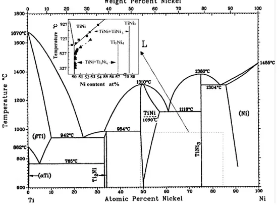
1.1.1 - Phase Diagram of the Ni-Ti System

(30)

6

has suffered some modifications along the time. NiTi is an intermetallic that, at low temperature, only exists in a very narrow band of compositions (near equiatomic).

Figure 1 – Phase diagram of a Ni-Ti alloy in which is highlighted the phase equilibrium between. [3]

The phase diagram allows us to notice the existence of a stability domain of the austenitic phase (B2). This domain is characterized, for Ni-rich alloys, by a strong variation of the solubility limit with the increase of temperature. For Ti-rich alloys this variation is very slight. At low temperatures the extension of the stability domain of the austenitic phase is practically nonexistent.

Generally, SMAs have two different phases, each one with different crystal structures and, as a consequence, with different properties. The high temperature phase is called austenite and the low temperature phase is called martensite. The transformation from one structure to another does not occur by diffusion of atoms but rather by shear lattice distortion. This kind of transformation is known as martensitic transformation. Each martensitic crystal formed can have a different orientation direction, called a variant. The assembly of martensitic variants may exist in two forms: twinned martensite, which is formed by a combination of “self -accomodated” martensitic variants, and detwinned or reoriented martensite in which a specific variant is dominant.

The reversible phase transformation from austenite, also known as parent phase, to martensite, or product phase, and vice versa, form the basis for the unique behavior of SMAs. [1]

(31)

7

phase could sometimes appear between austenite and martensite. That phase is called R-phase and has a trigonal structure.

Figure 2 – Crystal structure of B2 austenite (top on the left), B19 martensite (top on the right) and B19’

martensite (bottom). [3]

1.1.2 - Martensitic Transformation Temperature

Experimentally is known that the martensitic transformation temperature is strongly dependent on the composition and/or alloying elements. NiTi is not a line-compound with a fixed composition: it shows a certain capability to dissolve some excess of Ni in the Ni-rich side but cannot dissolve the excess of Ti as it is depicted in Figure 1 (almost vertical line on the Ti-rich side but Ni-Ti-rich side has some solubility, up to 6% at 1000 °C). [3]

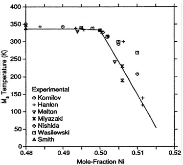
Figure 3 shows that the transformations temperature Ms is strongly dependent on Ni

concentration. However, in the Ti-rich side the transformation temperature is almost composition independent due to the fact that the solubility limit on NiTi in the Ti-rich side is practically vertical and thus is not possible to get rich Ni-Ti solid solution. This means that Ti-rich alloys will show a similar behavior as 50 at%Ni-Ti. On the Ni-Ti-rich side, an increase on the Ni content causes a drastic decrease of the transformation temperature Ms. Theoretically, this

(32)

8

Figure 3 – Transformation temperature as a function of Ni content for binary Ni-Ti alloys. [3]

1.1.3 - Phase Transformation in SMAs

As mentioned before the reversible transformation from austenite to martensite and vice versa are the basis for the unique behavior of SMAs.

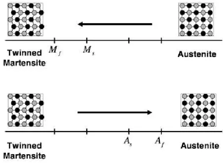
Upon cooling, and without any load applied, the crystal structure changes from austenite to martensite. This phase transition is called the forward or direct transformation. This transformation is due to the formation of several martensitic variants, which are up to 24 in Ni-Ti alloys. The arrangement of variants occurs in such a way that the average macroscopic shape change is negligible, resulting in twinned martensite. When heating from the martensite phase, there is a transformation of the crystal structure back to austenite, which is called reverse transformation. During this transformation there is no associated shape change.

The schematic of the crystal structure of twinned martensite and austenite for an SMA and the transformation between them is shown in Figure 4. During the forward transformation, without any load applied, austenite begins to transform to twinned martensite at the martensitic start temperature (Ms) and the transformation will be completed at martensite

finish temperature (Mf). At this point the material is fully twinned martensite. Upon heating,

the reverse transformation occurs at austenitic start temperature (As) and the transformation

is fully completed at austenite finish temperature (Af).

If a mechanical load is applied to the material in the twinned martensitic state it is possible to detwin the martensite by reorienting a certain number of variants (Figure 5). This detwinning process will induce a macroscopic shape change where the deformed configuration is retained when the applied load is released. A subsequent heating of the material above Af will cause a

reverse transformation from detwinned martensite to austenite which will lead to complete shape recovery (Figure 6). Cooling back to a temperature below Mf will lead to the formation

(33)

9

detwinning start stress (σs). The complete detwinning process will occur when the detwinning

finish stress (σf) is reached.

Figure 4 – Temperature-induced phase transformation of na SMA without mechanical loading. [1]

(34)

10

Figure 6 – Schema of the SME for an SMA. [1]

Since the forward and reverse transformations occur over a range of temperatures (Ms to Mf,

As to Af) for a given SMA composition, it is possible to construct transformation regions in the

stress-temperature space. The transformation temperatures strongly depend on the magnitude of the applied load, with higher values of applied load leading to higher transformation temperatures, as shown in Figure 7. Under an applied uniaxial load with a corresponding stress, σ, the new transformation temperatures are represented as Mσ

f, Mσs, Aσs

and Aσf for martensitic finish, martensitic star, austenitic star and the austenitic finish

temperatures, respectively.

Figure 7 – Temperature-induced phase transformation in the presence of applied load. [1]

1.1.3.1 - Superelasticity

(35)

11

Taking into consideration the Figure 8, it is possible to observe that, for a constant temperature above Af, it is possible to have the stress induced phase transformation from

austenite to martensite. This martensitic transformation is the basis of the superelastic effect. The load applied will give rise to a stress-induced martensite (SIM) with shape modification. It must be noticed that this martensite is detwinned martensite.

Figure 8 – Schema of superelastic effect. [1]

To illustrate the superelastic effect let us consider the cycling load presented in Figure 9. From A do B the parent phase undergoes elastic loading. Point B is the minimum stress level to start inducing the transformation from austenite to martensite (σMs_{). This transformation occurs}

because austenite becomes unstable and SIM starts to form. [5] Note that the stress-induced transformation from austenite to martensite is accompanied by generation of large inelastic strains as shown in Figure 9. From B to C the transformation from austenite to martensite proceeds and simultaneously martensite variants are being re-oriented, meaning that we can have both twinned and detwinned martensite, but at the end we will only have detwinned martensite due to the re-orientation of twinned martensite during this stage. At point C we reach the stress level where the martensitic transformation is over (σMf_{). From C to D there is}

the elastic loading of the detwinned martensite. By decreasing the stress applied during unloading, martensite will unload (elastically) from point D to E. Point E marks the beginning of the transformation from detwinned martensite do austenite (σAs_{). The reverse transformation}

(36)

12

Figure 9 – Typical SMA superelastic cycling load. [1]

The hysteresis loop represented in the σ-ε space represents the energy dissipated in the transformation cycle.

(37)

13

Figure 10 – Typical stress-strain curve for a fully austenitic NiTi SMA. [7]

Note that the stress-strain curve for a fully martensitic NiTi SMA (Figure 11) despite their similarities have some features that are very distinguishing. The main differences are that the plateau in the fully martensitic NiTi is reached for a minor stress level when comparing with fully austenitic NiTi, also the maximum strain achieved is lower for fully martensitic NiTi than for fully austenitic NiTi.

(38)

14

Figure 11 – Typical stress-strain curve for a fully martensitic NiTi SMA. [7]

Figure 12 shows the difference between the deformation mechanisms of stainless steel, which can accommodate higher stress by irrecoverable slip, and a superelastic NiTi alloy, which can accommodate higher deformation due to a reversible process by shifting to twinned martensite.

Figure 12 – Schematic representation of lattice changes in stainless steel and in a superelastic alloy. [8]

(39)

Stress-15

Strain curve is characterized by a closed loop), it is called PE, apart from its origin. PE is a generic term which encompasses both superelastic and rubber-like behavior. When a closed loop originates from a stress-induced transformation upon loading and the reverse transformation upon unloading, it is called SE. The rubber-like behavior occurs by the reversible movement of twin boundaries in the martensitic state. However, this singular behavior does not appear in Ni-Ti alloys. [9]

1.1.3.2 - Shape Memory Effect

SME was already introduced before. Here we present a more comprehensive explanation for this mechanical feature.

SME is a phenomenon such that even though specimen is deformed below As it regains its

original shape by heating up to a temperature above Af which leads to a reverse

transformation. The deformation imposed to the specimen could be of any kind such as tension, compression or bending, as long as the strain is lower than some critical value. SME occurs when specimens are deformed below Mf or at a temperature between Mf and As, above

which martensite becomes unstable. [9]

If we cool the sample to a temperature below Mf the martensite is formed in a

self-accommodating manner. In this process the shape of the specimen does not change due to the self-accommodated transformation. By applying an external force, the twin boundaries move in order to accommodate the applied stress. If the stress is high enough, one single martensite variant will be favored and shape of the specimens is altered. By heating up the sample above Af , the reverse transformation occurs, and, if this reverse transformation is crystallographically

reversible, the original shape is regained. Note that for SME to exist, it is necessary to fulfill two conditions: the deformation proceeds solely by the movement of twin boundaries and the transformation is crystallographically reversible. If either one of these conditions is broken, complete SME is not observed.

Figure 13 shows the microstructural changes that occur in NiTi martensite under stress and which are the basis for the SME. In stage a), we have twinned martensite; in stage b) with the increase of the applied stress, martensite starts to be detwinned; in stage c), continuing to increase the stress, martensite stays fully detwinned; finally, if stage d) is reached, there is no possible way to recover the initial shape of the specimen, since the deformation induced is permanent, due to dislocation slip. When stage c) is finished, it is possible to recover the initial shape of the specimens just by heating up to Af, having this way the SME.

(40)

16

If the specimen is deformed in a range of temperatures between Mf and As SIM also

contributed to the deformation, in addition to the above process of variant coalescence.

1.1.1.3 - Existence of Superelasticity and Shape Memory Effect

Despite the fact that SE and SME were discussed separately, they are closely related. Figure 14 shows the relationship between these two features. It is expectable that both SE and SME are observable in the same specimen, depending upon the test temperature and as long as the critical stress for slip is high enough.

Figure 14 – Schematic diagram representing the region of shape memory effect and superelasticity in temperature-stress coordinates; (A) represents the critical stress for the case of high critical stress and (B)

represents the critical stress for low critical stress. [3]

SE occurs above Af where martensite is completely unstable in the absence of stress. SME

occurs below Mf followed by heating up to Af. Between As and Af both occur partially. The

straight line with positive slope represents the variation with temperature of the critical stress to induce martensite, following the Clausius-Clapeyron relationship ( ). With the increase of temperature, a higher stress is required to induce martensite. The straight lines with negative slopes (A and B) represent the critical stress for dislocation slip. It is possible to manipulate the straight line A just by a softening effect in the material, which will lead to a drop of the line. On the other hand, due to a hardening effect, the same line could raise and with that it is possible to manipulate a certain window for some mechanical feature, such as SE or SME. Since dislocation slip never recovers upon heating or unloading, the applied stress must be between the lines in order to realize SE or SME. SE will not occur if the critical stress for dislocation slip is as low as the line B, since slip occurs prior to the onset of SIM.

1.2 - Laser welding

1.2.1 - Basic Laser Fundamentals

(41)

17

interaction/pulse time (10-3_{to 10}-15 _{s) on to any kind of substrate trough any medium. [10]}

Laser can be employed in many different fields such as metrology, reprography, military, medical, etc.

In laser welding the high power density used for materials joining leads to a formation of a hole due to evaporation. The hole formed is transverse through the material, with the molten walls sealing up behind it. This is known as the “keyhole” weld, which is normally characterized by its parallel sided fusion zone and narrow width. Figure 15, shows different fusion zone profiles for different welding processes.

Figure 15 – Different fusion zone profiles for different laser welding techniques. [10]

Since the weld is rarely wide compared with the penetration, it can be seen that the energy employed in the process is being used for melting the interface to be joined and not most of the surrounding area as well. A term that define the concept of efficiency is known as “joining efficiency”, which is defined as , where v is the travel speed (mm s-1_{), t is the thickness of}

the sample to be welded (mm) and P is the incident power (kW). The higher the value of joining efficiency the less energy is spent in unnecessary heating, which can lead to the existence of a wider heat affected zone (HAZ) or to distortion.

(42)

18

conduction the fusion zone (FZ) and the HAZ will be larger than in the keyhole mechanism (see Figure 16 to compare the effect of both mechanisms).

Figure 16 – Keyhole welding (on the left) and conduction-mode welding (on the right). [10]

It must be noticed that laser welding has many process parameters that need to be controlled in order to attain a good weld (Figure 17). Those process parameters are: beam properties such as power, pulsed or continuous laser, spot size and mode, wavelength; transport properties such as speed, focal position, joint geometries, gap tolerance; shroud gas properties such as composition and pressure; material properties such has composition and surface conditions.

(43)

19

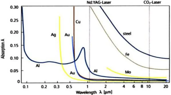
As depicted in Figure 18 metallic materials tend to absorb laser radiation, especially at wavelengths below 1 µm. Recent develops in laser industry has been the production of lasers with high power, low wavelength and good beam quality.

Figure 18 – Absorption of a number of metals as a function of laser radiation wavelength. [12]

Laser welding has some particular characteristics which are distinct from other welding processes. These characteristics are: high energy density, with a “keyhole” type weld, which causes less distortion; high processing speed and rapid start/stop; welds at atmospheric pressure; no filler required; narrow weld and relatively little HAZ, which means that laser welding can be used in near heat-sensitive materials; very accurate welding is possible; little or no contamination since protection gases can be used; relatively little evaporation loss of volatile components, which makes this technique very suitable for certain alloys such as Mg or Li alloys); relatively easy to automate the process. However some materials can be very difficult to join by this technique. For instance materials with high reflectivity (such as aluminum) can be difficult to join. Other disadvantages are the initial high cost of the equipment and the high cost with protection gases such as helium (He) or argon (Ar).

1.2.2 - Laser welding of NiTi

Due to the poor workability of NiTi alloys, suitable welding techniques must be used to obtain devices and components with different geometries. However the mechanical and functional behavior of these alloys is strongly influenced by possible thermal effects and modifications of the chemical composition associated with the welding process chosen. [13] There are not many joining techniques suitable for this class of materials. Among these techniques we have friction welding, resistance welding and tungsten inert gas (TIG). Laser welding is one of the most important joining techniques available for this class of materials. In particular the Nd:YAG laser, which was used to perform the similar NiTi joints, is suitable for welding low thickness components due to its high precision and reduced HAZ. [14]

(44)

20

mm thickness) [14], [20] is not as reported as the previous mentioned. Despite all the work done in similar welding of similar NiTi joints the effect in terms of the mechanical properties, chemical composition and therefore the phases present in the different parts of the welded specimens is not clear yet. In particular, the comprehension of the effect of long cycling in these materials is very important, in order to use this joining process with high reproducibility in NiTi SMA for several applications. Some cycling experiments regarding laser welded NiTi similar joints are presented in the literature, however these kind of experiments are characterized by a relatively low number of cycles (usually up to 20 cycles) and by low strain (up to 4%) achievements during the mechanical tests. One example of a cycling test with a slightly increase of the number of cycles (up to 30) and of the strain (up to 6%) was recently presented by Vieira et al. [21]

After welding the modifications introduced due to the laser processing tend to affect certain features over others. For instance, welded specimens tend to present lower ultimate tensile strength (UTS) and elongation to fracture. SME may prevail depending if the strain applied is not enough to induce an irreversible deformation of martensite. SE may have a greater or less extension depending on the chemical alterations that the FZ and the HAZ has suffered during the laser welding.

During welding, as mentioned before, the interaction of the laser beam with the material causes a localized fusion and in the neighboring regions there is a temperature increase without change of state.

In the FZ, if there is a preferential evaporation of one of the elements it may give rise to chemical composition changes. For the Ni-Ti system, it is expected that Ni has a higher evaporation rate than Ti (Figure 19). [22] Despite the existence of a shielding gas, these phenomena may still occur.

(45)

21

In the HAZ, if the temperature is high enough, full solution may occur and, depending on the cooling rate, precipitation phenomena may take place, or not. This precipitation will lead to a chemical composition change in the surrounding matrix.

It is possible that the chemical compositions changes that may occur in the FZ and in the HAZ, as mentioned above, may alter the transformation temperatures of the welded samples.

1.3 - Justification of the Work Developed

The work developed during this Master Thesis is the continuation of the work developed by Vieira. [23] On that work similar and dissimilar butt joints using NiTi were laser welded and studied in order to access how laser welding influences the mechanical and microstructural characteristics of the welds. It was used a laser power source operating in continuous mode.

For this reason some of the methods and experimental results attained by Vieira will be presented in order to justify the work done during this Master Thesis.

(46)

(47)

23

2 - Materials and Methods

2.1 - Materials

Similar NiTi/NiTi butt weld joints were joined using superelastic NiTi alloy (50.8 at% Ni) plates with 1.0 ± 0.1 and 0.50 ± 0.05 mm thicknesses from Memory-Metalle GmbH Alloy S (superelastic standard alloy). The alloys had an Af temperature of about 0 °C (according to the

manufacturer), were flat annealed and surface oxide free. The flat annealing gave to the samples its shape in the austenitic state.

Physical and mechanical properties of NiTi SMA are presented in Tables 1 and 2.

Table 1 – Physical properties of NiTi SMA [24]

Physical properties of NiTi SMA

Melting point

Density Specific heat

Coefficient of thermal expansion

Thermal conductivity

Martensite Austenite Martensite Austenite [°C] [kg/dm3] [J/kg.K] [x10-6 K-1] [W/m.K]

1300 6.45 322 6.6 11 8.6 18

Table 2 - Mechanical properties of NiTi SMA [24]

Mechanical Properties of NiTi SMA

Young modulus UTS Elongation Poisson

ration Martensite Austenite Cold

worked Fully annealed Cold worked Fully annealed

[GPa] [GPa] [MPa] [MPa] [%] [%] -

70-83 28-41 1900 895 5-10 25-50 0.33

2.2 - Welding Process

Similar NiTi/NiTi butt welds were produced using a Nd:YAG diode-pumped laser from Rofin-Sinar, model DY 033, in continuous wave mode available at Universidad Politecnica de Madrid premises. An ABB robot remotely controlled the laser head movement. The main characteristics of the laser equipment are displayed in Table 3.

All the laser welded joints were prepared and are described in the Master Thesis of L. Alberty Vieira. [23]

Table 3 – Technical data of DY 033 Rofin Sinar Nd:YAG laser [23]

DY 033 Rofin-Sinar Nd:YAG technical data

Wavelength 1064 nm

Maximum output power 3300 W

Number of cavities 6

Fiber diameter 400 µm

Optical arrangement

Title angle 3°

Focal length 160 nm

Beam diameter 0.45

(48)

24

Plates of 35x35x1.0 and 35x35x0.5 mm were butt joined. Fixing and alignment of 1.0 and 0.5 mm thick plates were achieved using a positioning system specially designed for this purpose. The system assures that opposite plates were in the same plane and tight to each other, due to small compressive force applied by the mechanism. He and Ar were used to create an inert atmosphere. Welding direction was perpendicular to the rolling direction.

Welding parameters of 1.0 and 0.5 mm butt joints are presented in Tables 4 and 5. [23]

Table 4 – Welding parameters for 1.0 mm butt joints [23]

Welding parameters for 1.0 mm thick plates

Sample reference

Power Welding speed

Heat input

FPP Focused beam Ø

Argon Helium Air knife Laterally Back [W] [mm/s] [J/cm] [mm] [mm] [bar] [l/min] [l/min]

A-A 990 25 396 0 0.45 7.5 40 50

B-B 990 20 495 0 0.45 7.5 40 50

C-C 990 15 660 0 0.45 7.5 40 50

D-D 1485 30 495 0 0.45 7.5 40 50

E-E 1485 25 594 0 0.45 7.5 40 50

F-F 1485 20 743 0 0.45 7.5 40 50

H-H 1980 40 495 0 0.45 7.5 40 50

Table 5 – Welding parameters for 0.5 mm butt joints [23]

Welding parameters for 0.5 mm thick plates

Power Welding speed

Heat input

FPP Focused beam Ø

Argon Helium Air knife Laterally Back [W] [mm/s] [J/cm] [mm] [mm] [bar] [l/min] [l/min]

F-F 726 30 242 0 0.45 7.5 40 50

K-K 790 50 158 0 0.45 7.5 40 50

O-O 858 70 122 0 0.45 7.5 40 50

After welding specimens were cut using a precision cut-off machine ATM GmbH model Brillant 211 equipped with a diamond wheel type B102 from the same maker. Cutting parameters were the following: speed - 4000 rpm; feed rate - 1 mm/min; lubricant - multipurpose cutting fluid.

(49)

25

2.3 –

Characterization Techniques

2.3.1 - Differential Scanning Calorimetry

Differential scanning calorimetry (DSC) is a thermoanalytical technique in which the difference in the amount of heat required to increase the temperature of a sample and reference is measured as a function of temperature. The sample to be analyzed and the reference are both kept at a same temperature during the experiment. [25]

A DSC 204 F1 Phoenix model from Netzsch was used in order to perform high and low temperature structural tests, using liquid nitrogen on low-temperature tests. DSC was used in order to characterize the base material (BM) in terms of zero-stress structural transformation temperatures. Liquid nitrogen was used to cool down the system to about -160 °C. Upon heating the maximum temperature was of about 70 °C. The cooling and heating rate was of 10 °C/min.

2.3.2 - Mechanical Tests

2.3.2.1 - Uniaxial Static Tensile Tests

Uniaxial tensile tests were performed on the samples welded by Vieira. [23] These tests were performed at room temperature, at CENIMAT, on an AUTOGRAPH SHIMADZU model AG500Kng equipped with a SHIMADZU load cell type SFL-50kN AG with a total capacity of 50 kN. UTS and elongation to fracture were recorded.

2.3.2.2 - Cycling Tests

Considering UTS and elongation to fracture of welded samples presented in Tables 7 and 8 an alternated cycling routine with a total of 5 sets of cyclic tests was developed. The 5 sets of cyclic tests chosen are presented in Table 6. The equipment used is mentioned just above.

Table 6 – Alternated cycling routine for the welded samples

Set of cyclic test Maximum strain Cycles

1 10 60

2 8 60

3 10 60

4 8 60

5 10 360

Number of total cycles if the sample did not break : 600

Sample K-K due to its mechanical properties (see Table 8) in stages 1, 3 and 5 was strained up to 9% instead of 10%.

If the sample tested would stand for the entire cycling routine it would stand to a total of 600 cycles. This kind of test, with the samples being subjected to very high strains during a large number of cycles, was not been reported in the literature yet.

(50)

26 2.3.3 - Shape Memory Effect Evaluation

The experimental method for evaluating the SME of the welded joints is based on bending and free-recovery testing, following previous work developed by Vieira [23], tests were performed by bending the sample in the martensitic condition followed by the removal of the load and heating up to the parent phase.

These tests were conducted using liquid nitrogen and a dedicated device manufactured in house (see Figure 21).

Figure 21 – Device used for testing the shape memory effect.

Tests were performed as shown in Figure 22. Note that the bending is performed when the sample is dipped in the liquid nitrogen and the recovery took place at room temperature. The results are expressed in terms of the Ω angle, which represents the permanent deformation angle. For example, if Ω = 0 it means that the sample recovered to its initial shape.

Figure 22 – Bending and free-recovery method used to analyze the shape memory effect of the welded samples.

(51)

27

investigate the influence of the angle between the rolling direction and the welding direction on the SME, it was used one sample with the rolling direction perpendicular to the welding direction (sample “Perpendicular”) and another one with both directions parallel to each other (sample “Parallel”). These samples were welded in the same conditions. Finally SME was evaluated in two samples with different thicknesses (0.5 and 1.0 mm, respectively samples K-K and F-F). All samples were tested four times, and the samples were positioned so that the face and the root of the weld bead were alternately submitted to tensile and compressive forces.

In order to assess if after the cycling tests the strain presented by the samples could be recovered, a different procedure was carried out. Samples B-B, C-C, F-F and K-K cycled 600 cycles, were dipped in the liquid nitrogen, bent and heated up above room temperature. Samples D-D and E-E were first heated up to around 70 °C and then were dipped in the liquid nitrogen, bent and heated up above room temperature. The heating of the samples before the dipping in liquid nitrogen was made to ensure that these samples before dipping had an uniform state (fully austenitic).

The 1.0 mm thick samples were subjected to a strain of 3.77% while 0.5 mm thick sample were subjected to 1.94% during SME evaluation.

2.3.4 - X-ray Diffraction Analysis

2.3.4.1 - Minor Introduction to X-ray Analysis

XRD is a tool for the investigation of the fine structure of matter. [26] This technique had its beginning in von Laue’s discovery in 1912 that crystals diffract x-rays, the obtained diffraction revealing the structure of the crystal. XRD is widely used for the determination of the crystal structure of materials, residual stresses, size of crystallites and preferential orientation of the grains in the analyzed material.

When a material is bombarded with x-rays of a fixed wavelength (which must be similar to the spacing of the atomic-scale crystal lattice planes) and at a certain incident angles, intense reflected x-rays are produced when the wavelengths of the scattered x-rays interfere constructively. In order for the waves to interfere in a constructive way, the differences in the travel path must be equal to integer multiples of the wavelength. When this phenomenon occurs, a diffracted beam of x-rays will leave the material at an angle equal to that of the incident radiation.

(52)

28

Figure 23 –Schematic representation of the Bragg’s law. [27]

The general relationship between the wavelength of the incident x-rays, angle of incidence and spacing between the crystal lattice planes of atoms is known as the Bragg’s law (proposed in 1913), which is expressed as: , where n is an integer (the order of the reflection), λ is the wavelength of the incident x-rays, d is the interplanar spacing of the crystal and Ѳ is the angle of incidence. [26]

2.3.4.2 - Experimental Set-up for the Base Material

XRD analysis of the BM was performed using a Bruker diffractometer (rotating anode – XM18H, Cu-Kradiation (1.5418 Å), 30 kV/100 mA, D5000 goniometer and TTK-450 chamber from Anton Paar) with conventional θ/2θ scanning at various temperatures from 120 to -180 °C.

2.3.4.3 - Experimental Set-up for the Welded Samples

(53)

29

Figure 24 – Scheme used for the XRD measurements.

The data acquired was treated with the software Fit2D [28], obtaining XRD patterns from the Debye-Scherrer rings. The Debye-Scherrer rings are two-dimensional patterns consisting in concentric rings produced by the superposition of reflections of various crystals where the x-ray beam is focused and that are oriented according to a (hkl) plane fulfilling the diffraction condition of Bragg. [26] Figure 26 is a schematic representation of the attainment of Debye-Scherrer rings.

Figure 25 – Schematic representation of the mode of obtaining the Debye-Scherrer rings.

For a complete randomness of orientations every crystallographic plane of that family make the same diffraction angle relatively to the incident beam, which leads to the formation of a diffracted beam with conic symmetry. The intersection of the cones with a plane perpendicular to the cones axis gives the Debye-Scherrer rings.

(54)

30

XRD technique was chosen to analyze the welded samples since the welding process can cause alteration in the phases present in the material. In particular, the welding procedure may alter the existing phases in the HAZ and in the FZ when comparing with the BM.

All welded samples were analyzed. In addition, two extra samples were studied, to examine the effect of the mechanical cycling on the microstruture: sample B-B after 4 and 600 cycles.

2.3.5 - Scanning Electron Microscopy

(55)

31

3 - Experimental Results

This chapter aims to present the experimental results. For this, a brief description of the mechanical properties of the laser welded specimens [23] that constituted the basis for the cycling tests performed is presented.

Regarding the work developed during this Master Thesis, the results are organized in the following sequence:

- DSC analysis from the as-received plates which allow determining the transformation temperature ranges of theBM.

- XRD measurements that allow the structural characterization of BM at different temperatures. Also, XRD patterns of the welded samples to characterize the weld bead and its neighboring regions, identifying, at room temperature, the different phases in each zone of the welded samples (namely in the HAZ, FZ and BM), with a fine spatial resolution, will be presented. From this XRD data, it is also possible to identify different microstructural features, such as preferential orientation or existence of fine or coarse grain.

- Mechanical tests from cyclic load/unload of the welded samples and a summary of the evolution of the accumulated irrecoverable strain with the number of cycles.

- Tests to assess the influence of the welding parameters on the SME in the welded joints.

- SEM analysis of samples A-A and C-C, to understand the fracture mechanism of the welded joints that suffered premature rupture.

When justified, a short summary of the results in appropriated Tables is given in order to facilitate the interpretation of the experimental results in the discussion chapter.

3.1 - Mechanical Properties of the Welded Samples

The strength and ductility parameters from tensile tests results for 1.0 and 0.5 mm thick samples [23] are presented in Tables 7 and 8, respectively.

Table 7 – Strength and ductility parameters from tensile test results of 1.0 mm thick samples [23]

Strength and ductility parameters from tensile test results of 1.0 mm thick samples

Sample reference UTS [MPa] Elongation to fracture [%]

A-A 637 12.1

B-B 511 10.6

C-C 530 11.1

D-D 482 10.1

E-E 337 6.5

F-F 522 11.3

G-G 439 10.4

H-H 501 11.5

(56)

32

Table 8 – Strength and ductility parameters from tensile test results of 0.5 mm thick samples [23]

Strength and ductility parameters from tensile test results of 0.5 mm thick samples

Sample reference UTS [MPa] Elongation to fracture [%]

F-F 585 10.7

K-K 367 8.34

O-O 519 10.2

3.2 - Differential Scanning Calorimetry

The phase transformation temperatures for a zero-stress condition measured by DSC on the BM are depicted in Figure 26, while Table 9 summarizes the transformation temperatures.

Figure 26 – DSC measurements of the base material for determination of the transformation temperatures

Table 9 – Summary of the transition temperatures of the base material

Transformation temperatures of the BM from DSC analysis

Ms [°C] Mf [°C] Rs [°C] Rf [°C] As [°C] Af [°C]

Upon heating - - - - -22 24

Upon cooling -53 -98 15 -12 - -

(57)

33

3.3 - X-ray Diffraction Analysis

3.3.1 - Analysis of the Base Material subjected to Thermal Cycling

Figures 27 depicts the XRD analysis of the BM from 120 to -180 °C, and Figure 28 shows the contour lines of Figure 27.

Figure 27 – XRD analysis of the BM from 120 to -180 °C (Cu-Kradiation, 1.5418 Å).

Figure 28 – Contour lines from the XRD analysis of the BM (Cu-Kradiation, 1.5418 Å).

(58)

34 3.3.2 - Analysis of the Welded Samples

3.2.2.1 - 1.0 mm thick samples

The XRD patterns along the samples A-A, B-B, C-C, D-D, E-E, F-F and H-H are depicted in Figures 29 to 37. For sample B-B there is also XRD patterns after 4 and 600 cycles, in order to access the microstructural modifications due to cycling tests. In 3D XRD graphs that will be now presented only austenite peaks are identified (with black arrows corresponding to a specific value of 2Ѳ), the remaining corresponding to martensite (no R-phase detected).

Figure 29 – XRD patterns along sample A-A (synchrotron radiation, 0.1426 Å wavelength).

(59)

35

Figure 31 – XRD patterns along sample B-B after 4 cycles at 10% (synchrotron radiation, 0.1426 Å wavelength).

(60)

36

Figure 33 – XRD patterns along sample C-C (synchrotron radiation, 0.1426 Å wavelength).

(61)

37

Figure 35 – XRD patterns along sample E-E (synchrotron radiation, 0.1426 Å wavelength).

(62)

38

Figure 37 – XRD patterns along sample H-H (synchrotron radiation, 0.1426 Å wavelength).

From Figures 29 to 37 it is possible to verify the existence of different phases in each of the major regions of a weld (BM, HAZ and FZ). For all samples in the BM there is only austenite, while in HAZ and FZ there is martensite and austenite, but with a major prevalence of martensite in the FZ when comparing to austenite.

Tables 10 summarizes how the relative amounts of martensite and austenite in the BM, HAZ and in the FZ vary amongst different samples with 1.0 mm thickness.

Table 10 – Summary of the existing phases present in different zones of the analyzed samples 1.0 mm thick

Summary of the existing phases and their relative amounts between samples welded with the same laser power

Samples A-A, B-B and C-C

All samples have martensite and austenite in the FZ. Sample A-A has a higher amount and sample C-C the lower amount of martensite. In the BM there is

only austenite. Samples D-D,

E-E and F-F

Sample D-D and E-E have approximately the same amount of martensite, with a slight increase for sample E-E. Sample F-F has a lower amount of martensite than samples D-D and E-E. In the BM there is only austenite.

Sample B-B after 4 and 600 cycles presents a higher amount of martensite in the HAZ and in the FZ when comparing with sample B-B without any mechanical cycle. Sample H-H had also martensite and austenite in the weld bead with a greater prevalence of martensite.

3.2.2.2 - 0.5 mm thick samples

(63)

39

Figure 38 – XRD patterns along sample F-F (synchrotron radiation, 0.1426 Å wavelength).

(64)

40

Figure 40 – XRD patterns along sample O-O (synchrotron radiation, 0.1426 Å wavelength).

For 0.5 mm thick samples there is also only austenite in the MB, while HAZ and FZ both have martensite and austenite. As it will be discussed later for these samples there is no possibility to make a reasonable comparison between the relative amounts of martensite existing in each sample.

3.4 - Cycling Behavior

3.4.1 - 1.0 mm Samples

3.4.1.1 - Cycling Tests

The results obtained from the cycling tests performed on 1.0 mm thick samples are summarized in Table 11.

Table 11 – Summary of the cycling tests performed on 1.0 mm thick welded samples

Summary of the cycling tests performed on 1.0 mm thick welded samples

Rupture at

Number of test set Cycle number Total cycles Where

A-A 5 61 301 Base material

B-B No rupture - 600 -

C-C No rupture - 600 -

D-D No rupture - 600 -

E-E No rupture - 600 -

F-F No rupture - 600 -

H-H 1 45 45 Weld bead

(65)

41

Figure 41 – Cycling test of sample A-A.

(66)

42

Figure 43 – Cycling test of sample C-C.

(67)

43

Figure 45 – Cycling test of sample E-E.

(68)

44

Figure 47 – Cycling test of sample H-H.

The cycling tests show that, for all samples, there is a convergence of the hysteretic loops from the first cycle to the last one of each cycling test. The superelastic plateau is clearly defined on the first set of the tests performed. On the following sets of the cyclic tests this plateau is not as evident as it was on the first set, though it is still present.

There is also a decrease in the stress of the SIM and reverse transformation with the increase of the number of cycles. This decrease is larger in the SIM transformation than in the reverse transformation.

(69)

45

Figure 48 – Zoom from the beginning of the cycling test of sample B-B to show the existence of R-phase.

The irrecoverable strain after the first cycle is higher than 2% for all samples, except for sample H-H where it is lower than 1%.

3.4.1.2 - Accumulated Irrecoverable Strain

As it can be depicted on the cycling tests presented above the accumulated irrecoverable strain with the number of cycles of each sample differs. Table 12 summarizes the final value of accumulated irrecoverable strain at the end of the cycling test performed. During the “Discussion” section, several Figures with the evolution of the accumulated irrecoverable strain with the number of cycles will be presented in order to facilitate the interpretation of the results attained.

Table 12 – Summary of the accumulated irrecoverable strain after the cycling test for 1.0 mm thick samples

Summary of the maximum accumulated irrecoverable strain

Sample Number of cycles Accumulated irrecoverable strain after the cycling test [%]

A-A 301 5.01

B-B 600 8.62

C-C 600 9.21

D-D 600 9.01

E-E 600 8.99

F-F 600 7.21

H-H 45 1.93