UNIVERSIDADE DO ALGARVE
Faculdade de Ciências e Tecnologia, Campus Gambelas
Centro de Ciências do Mar & Centro de Investigação Marinho e Ambiental
COMPARING ZOSTERA AND SPARTINA ENVIRONMENTS
IN RELATION TO CARBON BURIAL: A SEDIMENTARY
AND GEOCHEMICAL APPROACH FROM RIA FORMOSA.
Natalia Duque Núñez, a4870
Master's thesis
Master integrated in marine biology
Work performed under the guidance of:
Dra. Cristina Veiga – Pires and Dr. Rui Santos
.FARO 2015
COMPARING ZOSTERA AND SPARTINA ENVIRONMENTS
IN RELATION TO CARBON BURIAL: A SEDIMENTARY
AND GEOCHEMICAL APPROACH FROM RIA FORMOSA
Declaração de autoria de trabalho:
Declaro ser autor deste trabalho, que é original e inedito. Autores e trabalhos consultados estão devidamente citados no texto e constam da listagem de referências incluida.
Copyright:
A Universidade do Algarve tem o direito, perpétuo e sem limites geograficos, de arquivar e publicitar este trabalho através de exemplares impressos reproduzidos em papel ou de forma digital ou por qualquer outro medio conhecido ou que venha a ser inventado, de o divulgar através de repositorios cientificos e de admitir a sua còpia e distribução com objetivos educacionais ou de investigação, não comerciais, desde que seja dado credito ao autor e editor.
“The important thing is not stop questioning. Curiosity has its own
reason for existing”
Acknowledment
ACKNOWLEDGEMENT
Firstly would like to thank Professor Rui Santos for this support, coordination and positive comments, as well as his teaching in some of the courses he lectured and Professor Cristina Veiga-Pires, whose dedication to this study as well as her support, orientation, advices and friendship have been one of the keys for the success of this study.Thank you both for giving me this opportunity to wave great work I would also like to thank Paulo Santana for his support and help he has provided during the laboratory analyses. I would to mention to Isabel Barrote, Monya M Costa, Ana Alexandre and whole team of ALGAE for the priceless help they have offered me, for letting me part of the team and the good moments we have spend at work. I would like mention personally Fernando Canovas for this orientation, dedication and help, as well as, his friendly. Also want to thank Gianmaria Califano for the sampling collection. Furthermore thank to Vera Gomes for her help during the laboratory analyses of elemental composition.
In general thank you so much to all! I still have many things to learn from you. Thank to increase my interest in the science!
With respect to my “Familia gaditana”,i cannot forget to thank Emilio, Pablo, Isma, Vito, Susi, Canto, Sara, Helena, Mikel, Borja, Miguelito , Dani, Dani rastas and Laura “chochi”. Thank to all of you and those that i am not mentioning for yours friendship and for all the incredible moments and adventures that we have spend together, I would love to travel back in time!!! Part of this family went with me on the adventure of two years in Faro, and I have to thank to Peter, Laura, Sofi and Claudia , as well as Jorge and David for the great moment, friendship, support and help, thank for making me feel at home anywhere. Now where are we going?
Especially, Cucus, thanks for always being my inexhaustible battery and trust me, and Lau thanks to be my wings in this very special years two years, my sisters, I feel lucky! Also i want to thank to my family Angola, Nelson and Domingas. Not to forget my abulense team Bea, Javi, Chory, Mireya, Sandra, Marta, Laura and Puy, whose huge friendship is not affect by the distant. I also want to thank Fuen and Marta for supporting me unconditionally.
Finally, I would to mention to a very special person to me, thank for all the moments and experiences that we have live together and for you help, support and love. Thank for all Javier Gamero! Asqueroso!
I do not to finish without highlighting the two people most important of my life my mother and my sister. It would not have been possible without them. Mom Thanks for helping me, always take care and support me in all my decisions and always lead me to my happiness unconditionally. Ainhoilla, simply, Thank you for existing! We are the best team of three! I love you so much!
I cannot feel more grateful to have had you support Thank you so much everyone! For my mum. THANK!
Resumo
I RESUMO
Os sumidouros de carbono são reservatórios naturais ou artificiais, nos quais o carbono pode ser acumulado durante um determinado período de tempo. Mangais, sapais, salinas e pradarias marinhas são habitats que têm um papel importante no balanço de carbono dos oceanos e, assim, influenciam o ciclo oceânico. Eles representam um hotspot mundial para armazenamento de carbono orgânico (OC). Estes habitats compartilham uma parcela excessiva no sequestro de C em relação aos habitats terrestres. Este OC pode ser encontrado na biomassa viva especialmente enterrada nos sedimentos. A acumulação de OC em sedimentos marinhos fornece armazenamento de C a longo prazo. Esta acumulação OC é influenciada por alguns parâmetros ambientais, tais como, por exemplo, a distância ao continente e/ou o tamanho de grão e pH, assim como o tipo de ambientes de marés.
Devido à falta de dados de deposição de carbono na área de estudo e também para destacar a importância destes ecossistemas no sequestro de carbono, neste estudo pretendeu-se avaliar "sumidouros de C" em relação a estes parâmetros ambientais tais como, por exemplo, a hidrodinâmica marinha relativamente à distancia ao continente, ou o sedimento, relativamente ao tamanho do grão nas diferentes estações de amostragem. Adicionalmente, dois diferentes ecossistemas intertidais da Ria Formosa, Zostera noltii vs Spartina marítima, foram avaliados. Esta abordagem multidisciplinar e integrada inclui análises biológicas, geológicas e químicas, para melhor compreender os processos que conduzem à acumulação de carbono, conservação ou degradação.
Para tal, foi realizada uma amostragem ao longo de um canal principal e um canal secundário da Ria Formosa, em quatro estações diferentes, sendo que em cada estação os dois ecossistemas foram amostrados. No laboratório, analisámos as características sedimentológicas, onde foi determinado o tamanho das partículas por difração laser e por uso de peneiros, com o obejctivo de estimar o nível relativo de energia presente no ambiente onde o sedimento foi transportado e depositado. A cor dos sedimentos foi analisada em todo o espectro de luz visível por reflectância difusa, permitindo-nos adquirir uma aproximação da composição do sedimento. Também foi estudada a composição mineralógica por difração de raios-X. Por outro lado, foram analisadas as características geoquímicas, o que incluiu a determinação da matéria orgânica e carbonato perdidos por
Resumo
II
combustão, análise de composição elementar (OC, IC, IN e ON) através de um sistema de combustão elementar e o raio de C/N foi calculado, para ter uma ideia aproximada da origem ou fonte da matéria orgânica. Também foi determinada a concentração de pigmentos, onde por um lado foram analisadas as concentrações de clorofila e carotenóides, usando uma extração simples com acetona e medidas as concentrações através do espectrofotómetro. Seguidamente, através de cromatografia HPLC, foram analisados os pigmentos específicos. Os resultados destas últimas análises foram, no entanto, não representativos, uma vez que os valores obtidos apresentavam artefactos de degradação, não tendo sido considerados.
O processamento de dados foi realizado utilizando o software estatístico R. Todas as propriedades físicas e bioquímicas de sedimentos foram avaliadas para cada estação e para cada tipo de habitat, avaliando a sua variabilidade. Um estudo ANOVA de dois fatores, sendo um de eles ‘estação’ e o outro ‘tipo de comunidade biológica’, foi aplicado a cada variável, de modo a saber se houve ou não diferenças significativas dependentes de cada fator individualmente ou devido ao efeito da interferência de ambos. Nos casos em que se verificaram diferenças, foi usado um post-hoc para determinar a origem da diferença, neste caso usamos o teste de Tukey. O software Gradistat, foi utilizado para calcular o cálculo estatístico do tamanho de grão.
Nos resultados em relação às características sedimentológicas, o tamanho da partícula reflete um gradiente em que o tamanho do grão nas amostras diminui à medida que nos afastamos do canal principal e nos aproximamos das estações do canal secundário. Este gradiente é mais marcado no caso da Z. noltii do que no da S. maritima. Esta diferença na intensidade do gradiente entre ambos ambientes pode ser devido às diferenças de hidrodinamismo entre os dois meios, uma vez que a Z. noltii está mais exposta que a S. maritma devido à sua posição no intertidal. Relativamente aos resultados de cor, foi observada a possível presença de várias formas de Fe e goetita devido aos tons do sedimento, apresentando um aumento em ambos os valores ou aumentado o conteúdo dessas substâncias da estação 1 para a 4 para ambos os ambientes. No composição mineral verificaram-se diferenças entre o teor de quartzo e polissilicatos entre as estações, aumentando o conteúdo de polissilicatos e redução do teor de quartzo nas estações mais
Resumo
III
protegidas. Também a presença de pirita e siderita poderia explicar os altos valores de matéria orgânica, ao proporcionar um possível ambiente redutor.
Um grande conteúdo em carbonatos foi encontrado na estação 4, podendo explicar-se devido à possível preexplicar-sença de foraminíferos. Em relação ao explicar-sequestro dos carbonos, é influenciado por praticamente todas as variáveis estudadas, já que influenciam as características do solo, favorecendo ou desfavorecendo a acumulação de carbono. Como por exemplo a presença de determinados compostos minerais ou substâncias que foram determinadas na análise da composição mineral e cor, que favorecem a agregação de matéria orgânica, ou outras resultando em condições reduzidas permitindo que ocorra uma maior acumulação no sedimento. Nem todas as variáveis mostram o mesmo padrão ou tendência relativamente às estações ou ao tipo de comunidade biológica. Para todas as variáveis estudadas neste trabalho, apenas algumas delas não apresentaram variações em ambos os fatores estudados. A melhoria destas representam diferenças entre estação e entre ambientes e mais da metade respondem à interação deles. Atendendo ao objetivo principal deste estudo, foram encontradas diferenças significativas entre os dois ambientes, mostrando a S. maritima aproximadamente o dobro do conteúdo de carbono do que a Z. noltii. Esta variabilidade foi relacionada com o tamanho do grão, observando-se uma relação positiva entre a concentração de carbono orgânico e a presença de sedimentos mais finos. Todos os fatores encontram-se influenciados pela composição do solo e hidrodinâmica. Finalmente, quando foi calculada a taxa da acumulação do carbono, S. maritima acumula dobro do que a Z. noltii, com resultais de valores de 131.8 g OC.m -2
.year-1, 83.9 g OC.m-2.year-1, respectivamente. Estas diferenças foram relatadas pela influência de todas os parâmetros analisados em este estudo.
Chaves palavras: Zostera noltii, Spartina maritima, Ria Formosa, sumideiro de carbono, carbono orgânico, taxa da acumulação do carbono.
Abstract
IV ABSTRACT
Carbon sinks are natural or artificial reservoirs in which carbon can be accumulated for a certain length of time. Mangroves, salt marshes and seagrasses beds are habitats that have an important role on the carbon budget of the oceans and thus influence the oceanic cycle. In this study we aimed is to evaluate C storage capacity of two different intertidal environments, Zostera noltii vs Spartina maritima from Ria Formosa, as well as to evaluate the influence of hydrodynamics and sediment grain size in the C storage. This multidisciplinary and integrated approach includes biological, geological and chemical analyses in order to better understand the processes leading to Carbon accumulation in sediments. For such a purpose, we analyzed and measured the granulometry, color and mineral composition of the sediment, as well as the organic matter, calcium carbonate contents and the elemental composition. The results obtained reflect that the carbon sequestration (organic carbon content), is related to practically all the studied variables, Furthermore, there are significant differences between both biological communities. S. maritima shows nearly twice the organic carbon content than Z. noltii. On the other hand, the distance to the main navigation channel, a proxy to hydrodynamics, affected all parameters, strongly affected C accumulation, with higher variability in Z. noltii than S. mariima. C accumulation and sediment grain size were related to this gradient, as expected, where both parameters increased from the first station, close to the main channel, to last station the most remote. The carbon accumulation rate for S. maritima environment was twice as high as those for Z. noltii environment, 131.8 g OC.m-2.year-1, 83.9 g OC.m
-2
.year-1, respectively, these differences were related to the influence to all the parameters analyzed in this study.
Keys words: Zostera noltii, Spartina maritima, Ria Formosa, carbon sink, organic carbon, carbon accumulation rate.
INDEX
1. Introduction……….……… 1
1.1. Carbon cycle in marine systems………... 1
1.2. Characterization of the Ria Formosa………... 5
1.3. Objective of the present study………... 6
2. Material And Methods……….... 8
2.1. Sampling sediment in the Ria Formosa………..… 8
2.2. Laboratory work………...… 10
2.2.1. Sediment Analysis………...… 12
2.2.1.a. Sediment granulometry by laser counting and sieving……... 12
2.2.1.b. Diffuse Reflectance Spectroscopy for color determination………...….... 13
2.2.1.c. Mineral identification……… 14
2.2.2. Geochemical Analysis………... 16
2.2.2.a. Determination of Organic matter and carbonate contents by Loss of Ignition………...…... 16
2.2.2.b. Determination of Elemental composition: OC, IC, ON, IN and C/N………...….. 17
2.2.2.c. Determination of Pigment contents………... 18
2.2.3. Statistical Analysis……….. 20
3. Result……….... 21
3.1. Sediment Analysis………. 21
3.1.1. Sediment granulometry by laser counting and sieving…..…... 21
3.1.2. Diffuse Reflectance Spectroscopy for color determination…... 25
3.1.3. Mineral identification………... 28
3.2. Geochemical Analysis………. 29
3.2.1. Determination of Water, Organic matter and carbonate contents by Loss of Ignition………...………..…. 29
3.2.2. Determination of Elemental composition: OC, IC, ON, IN
and C/N………... 32
3.2.3. Determination of Pigment contents………..37
3.3. Summary Result……….. 37 4. Discussion………...… 39 4.1. Sediment characterization………...……… 39 4.1.1. Sediment Analysis………..… 39 4.1.2. Geochemical Analysis………. 42 4.2. Carbon sequestration………... 46 5. Conclusion………....…. 48 6. References……….….... 50 Annexes………...….. 55
INDEX FIGURES Pag.
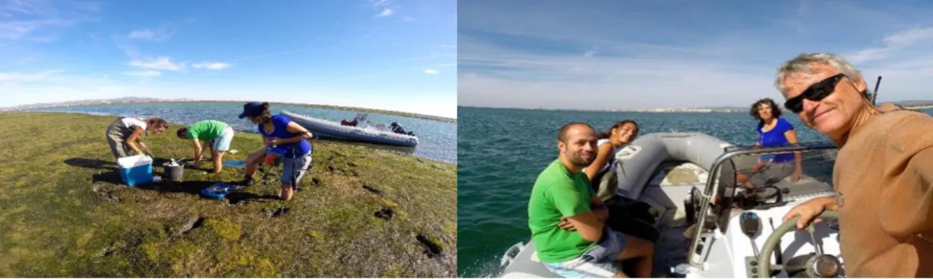
Figure 2.1: Sampling sediments in the Ria Formosa in a Z. noltii zone (left) and
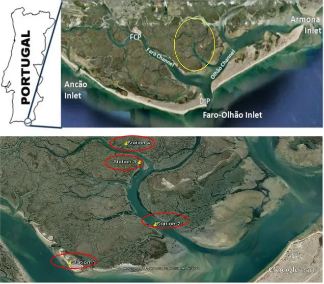
transportation between stations (right)... 8 Figure 2.2: Sample location of the Ria Formosa lagoon on the south coast of
Portugal (upper image). The stations were numbered Station 1 to Station 4. Image
obtained from Google Earth (lower image)……… 9
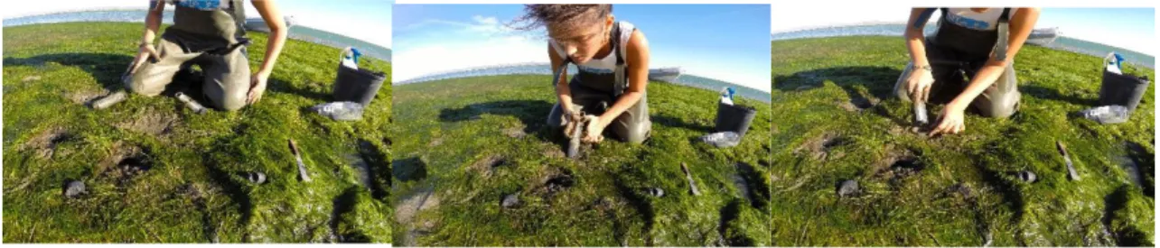
Figure 2.3: Photos of the sampling method with syringes showing one replicate
sampling with several holes……… 10
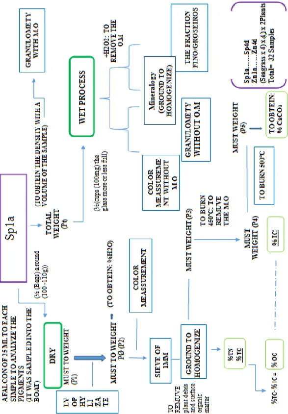
Figure 2.4: Process scheme followed for each of the sample. The example is with
Sp1a sample that is the “a” replicate of the sample retrieved at station 1 from S. maritima
environment………..
11
Figure 2.5: Picture showing the Mastersize 2000 model APA of 2000 of ©Malvern
Instruments Ltd……… 12
Figure 2.6: Sediment granulometry by the sieving process for evaluating the coarse
grain ratio……… 13
Figure 2.7: Full X- Ray Diffractometer “X´pert” (left) and its autosampler (right)….. 15 Figure 2.8: The figure shows the process carried out for each sample for
mineralogical analysis as described in the text, namely: the grounding equipment, the two containers and resulting wet fine sediment, the drying petri dishes in the oven
and the agate mortar……… 15
Figure 2.9: Homogenization process using a ball mill (FRITSCH, planetary micro
mil, pulverisette 7): Agate containers with balls (left), ball mill equipment (center),
resulting powders (right)………. 16
Figure 2.10: The Cosech 410 Elemental Analyzer……… 17
Figure 2.11: Pigment extraction process: samples protected against direct light (first
image), acetone addiction (second), vortex (three) and sonication process (fourth)….. 18 Figure 2.12: Spectrophotometer UV- Visible, Beckman Coulter, Du 650………….... 19 Formula 2.1: Reaction of combustion process for Carbon, Hydrogen, Nitrogen and
Formula 2.2: Equation to calculate organic carbon as, the difference between total
carbon and inorganic carbon………... 18
Figure 3.1: Percentage (% dw) Clay Mineral in function of sampling station for each
species………. 21
Figure 3.2: Percentage Fine/Coarse in function of sampling station for each species... 22 Figure 3.3: Rplot correlations between the Clay content from the sediment without
organic matter (“Mineral Clay”) and fine/coarse ratio in Z. noltii ……….. 22
Figure 3.4: Rplot correlations between the Clay content from the sediment without
organic matter (“Mineral Clay”) and fine/coarse ratio in S .maritima………… 23
Figure 3.5: Grain size ternary diagram for sediment classification (Folk 1954)
showing the classification schemes for Z. noltii (A) and S. maritima (B) based on the relative percentages of sand, silt and clay. The numbers inside of the blue circle
indicate the stations...………. 24
Figure 3.6: a* color for samples with organic matter in function of sampling station
for each species………... 25
Figure 3.7: a* color without organic matter in function of sampling station for each
species………. 26
Figure 3.8: b* color without organic matter in function of sampling station for each
species………. 27
Figure 3.9: Pattern of X-ray diffractometer for all the samples sample………... 29 Figure 3.10: Water content (% ww) in function of sampling station for each species. 30 Figure 3.11: Organic matter content (% dw) in function of sampling station for each
species………. 31
Figure 3.12: Carbonate content (% dw) in function of sampling station for each
species………. 32
Figure 3.13: Organic Carbon content (OC % dw) in function of sampling station for
each species………... 33
Figure 3.14: Organic Nitrogen content (ON % dw) in function of sampling station
for each species………... 34
nitrogen (% dw ON) to S. maritima environments………... 34 Figure 3.16: Rplot correlations between organic carbon (% dw OC) and organic
nitrogen (% dw ON) to Z. noltii environments……….. 35
Figure 3.17: Inorganic Nitrogen content (IN % dw) in function of sampling station
for each species………... 35
Figure 3.18: Inorganic Carbon content (IC % dw) in function of sampling station for
each species………. 36
Figure 3.19: C/N rate in function of sampling station for each species……… 37 Table 3.1: Mineral composition (%) for each station in function of sampling station
for each species………... 28
Table 3.2: Summary result (with/without differences to each variable) with respect
both factors (Distance to the continent/ Hydrodynamics, i.e., station vs type of
environment/biological community)……….. 38
Figure 4.1: Hjulström Diagram of transport and deposition for particles for different sizes,
regarding the average current speed (cm/sec) (Friedman et al., 1992) Blue circle: Approximation of current speed to stations 3 and 4; Green: Approximation of current speed to stations 1and 2……….... 40 Figure 4.2: Carbon accumulation rate (g. m-2. year-1) in function of sampling station
SYMBOLS, ABBREVIATIONS AND ACRONYM
Organic matter: OM.
Calcium carbonate: CaCO3.
Carbon dioxide: CO2.
Carbon: C.
Organic, inorganic and total carbon: OC, IC and TC.
Organic, inorganic and total Nitrogen: ON, IN and TN.
Hydrogen potential: pH.
Degrees Celsius: ºC.
Sodium Polyphosphate PRS: (NaPO3 ) n
Hydrogen peroxide: H2O2.
Diffuse reflectance spectrophotometry: DRS.
Visible spectrum: VIS spectrum
X-ray diffraction: XRD.
Angle: θ. Wavelengths: λ. Weight total: P total.
Samples weight before to liofilizate: P1.
Samples weight after to liofilizate: P2.
Vegetation weight: P3.
Samples weight before to burn: P4.
Samples weight after to burn at 950ºC: P6.
Carbon, Hydrogen, Nitrogen, Sulfur and oxygen: CHNS-O.
Thermal conductivity detector: TCD detector.
Hydrogen molecular or dihydrogen: H2.
Nitrogen molecular or dinitrogen: N2.
Oxygen diatomic: O2.
Carbon monoxide: CO.
Carbon tetrahydride (Methane): CH4.
Hydrogen hydroxide (Water): H2O
Sulfur oxide: SO x.
Ion of “x” element: X-. Nitrogen oxide: NO x.
Carbon, Hydrogen and Nitrogen: CHN.
A revolution per minute: rpm.
Chlorophyll derivatives: CD.
Total carotenoids: TC.
Analysis Of Variance: ANOVA.
Particle size distribution classification: PSDC.
Station 1- 4 in the environment of Z. noltii replicates” a- d”: Zn1a…Zn4d.
Introduction
1 1. Introduction
1.1. Carbon cycle in marine systems.
The carbon cycle has two important parts. One part is the biological pump, i.e. redistribution of biologically active elements such as carbon, nitrogen and silica in the ocean waters and the second part is the removal of these by deposition and burial in sediments. The formation of organic matter (OM) and calcium carbonate (CaCO3) allows
part of the carbon that is fixed by plankton to sink toward the deep ocean and is stored and buried for long periods of time before returning to the atmosphere (Sanchez et al., 2013).
This accumulation and sequestration of carbon is known as biological carbon sink, whenever CO2 emission is lower than its inputs (Diaz., 2014). The ocean is considered an
important carbon sink, which is referred commonly as Blue carbon (Nellemann et al., 2009). The publication of the Blue carbon report by Nellemann and co-authors (2009) showed the importance of the marine ecosystems in carbon sequestration. Coastal Marine ecosystems such as Mangroves, saltmarshes and seagrass beds particularly show an elevated carbon sequestration with relation to their global area (Laffley and Grimsditch, 2009). Recent data estimates that these ecosystems are responsible for capturing up to 70% of the organic carbon from the marine environment (Nellemann et al., 2009). These ecosystems have a great capacity to sequester and store important amounts of carbon in their sediments. About 20% of the global carbon sequestration is retained by these ecosystems despite occupying only 0.1% of the ocean surface (Duarte et al., 2013).
Seagrass meadows bury carbon at a rate 35 times greater than the terrestrial ecosystems e.g. the tropical forests (McLeod et al., 2011). Furthermore, there is a difference between the accumulation time of carbon in the terrestrial forests when compared to seagrass meadows, ranging from decades to thousands of years respectively (Macreadie et al., 2014). These ecosystems are adapted to marine life and can be found both permanently or temporarily submerged (Duarte et al., 2013). They provide many ecosystem services. For example, tidal salt marshes protect coastal fisheries of physical energy of the sea and provide shelter for juvenile fish. They provide valuable habitat for a lot of plants, birds and others animals, whose can serve as food resources. They also
Introduction
2
provide services and supplies to recreational hunters and fisher, many of which can give indirect economic benefits. They also offer protection from storm surges (Chmura., 2013).
With respect to the accumulation of carbon in seagrass meadows, it is due to breaches, stems and leaves (above-ground biomass), roots (below-ground biomass), and litter and dead wood (non-living biomass) (Grimsdith et al., 2013), as well as to sedimentary organic and inorganic constituents such as bacteria, microalgae, macro algae, detritus and carbonates respectively (Macreadie et al., 2014). This carbon is stored over millennia in the sediments. In addition, like the sea level rise, their sediments continue to accrete vertically, and hence do not become saturated with organic carbon; unlike terrestrial ecosystems that reach soil carbon equilibrium with time (centuries or millions of years) (Grimsdith et al., 2013).
Another explanation of the high carbon storage capacity of these environments is their capacity of acting as particulate traps. They develop large canopies that affect the flow of water existing above them, which in turn can modify their environmental abiotic conditions. One consequence of this develop of canopies is the accumulation of sediment and decreasing the resuspension of particles in the background. The formation of these canopies favors effectiveness of benthic subtracts, increasing the deposition surface of the sediment and probability of contact. Another characteristic that increases carbon accumulation is the presence of epiphytes on the leaves, because they increase the roughness of the leaves (Duarte et al., 2013). Thus, the coastal marine sediments are extremely rich and contain the majority of blue carbon (Grimsdith et al., 2013).
To understand this capacity to sequester and store of carbon in the sediment of theses ecosystems, it is important to define carbon stock in an ecosystem, as the amount of carbon stored, which is altered by having accumulation or release carbon in that ecosystem (Macreadie et al., 2014). For example, the accumulation of carbon as carbohydrates in the rhizomes can be used by the plant for respiration, or released in the sediments, where the secondary microbial production is supported. The carbon structure of the leaves is decomposed by bacteria and recycled by seawater. These two forms of carbon accumulation have a short residence time and thus cannot be considered part of the carbon stock. However, as the roots and rhizomes carry out their growth in the sediments under
Introduction
3
anoxic conditions, they have a low nutritional value for the bacteria (Macreadie et al., 2014). This low interest is due to the low concentration of nutrients (nitrogen and phosphorus) in their tissues (Duarte et al., 2013), so their decomposition is very slow and thus they accumulate in the sediments along large periods of time and can hence be considered as part of the carbon stock (Macreadie et al., 2014). Some authors have defined that 80% of the production of seagrass is not consumed by herbivorous and the rate of decomposition of this detritus is very low (Duarte et al., 2013). In terms of environmental factors affecting C capture and storage by seagrass, Macreadie and co-authors (2012) proposed some effects such as that of altered physical-chemical states on remineralization rates and the role of bioturbation fauna in facilitating mechanical flux of buried C out of sediment (role of microbial communities, also known as early diagenesis).
In summary, the high carbon storage capacity of seagrass has been explained because of its high primary production, its high capacity to filter out particles from water column and its high sediment retention capability. All this combines with a slow rate of decomposition in a seagrass environment low oxygen sediment and the lack of fires underwater (Fourqurean et al., 2012).
On the other hand, there is also an important variation in the carbon capture and storage between species. Carbon sequestration will vary according to their different rates of primary production, their ability to trap allochthones carbon through their canopies, the recalcitrance of the OC in their organs and in accordance with the characteristics of its preservation in sediments. In addition, the sp-habitat interactions influence carbon sequestration such as latitudinal, habitat ranges of temperature variations, sediment type, respiration in the sediment and remineralization (Labery et al., 2013). For example, the biochemical composition of the cell wall and other exterior cellular components among the seagrass meadows are probably different when looking at a high detailed level. These differences may require changes in microbial enzymatic processes of different dissimilative bacteria or fungi (Zak et al., 2006). In fact, one sediment profile can result from both aerobic and anaerobic processes. Different suites of microbes and microbial digestive systems may occur depending on the ecology of habitats, with differences between tropical and temperate habitats (Hoppe et al., 2002). Therefore, the integration of
Introduction
4
different environmental, chemical and biological factors is of fundamental importance in order to decipher their influence on the carbon storage capacity of seagrass. Understanding the causes for the high capacity of seagrass to capture and store carbon is fundamental to manage these ecosystems. Therefore, the seagrass may be even more important to the oceanic C cycle than previously considered (Fourqurean et al., 2012).
During recent times, close to 30% of seagrass area worldwide has been destroyed (Waycott et al., 2009), which is a major loss of C sink. Increasing the concern of large C leaks to the atmosphere, and thus accelerating climate warming. Current global rates of global loss of these ecosystems are calculated to be 0.7–2% per year (Grimsdith et al., 2013), among the highest rates of any ecosystem on the planet. This loss of seagrass C stocks, like terrestrial environments, is also due to anthropogenic disturbances either directly or indirectly. Indeed, sediments can be dredged, but the most common cause of seagrass disappearance is the degradation of water quality (Fourqurean et al., 2012). Thus, when these ecosystems are degraded or destroyed, large emissions of carbon dioxide are produced. This source of carbon dioxide is caused by the oxidation of carbon in biomass and organic content of sediment. This process occurs in the decade after the disturbance, but continues with the continuous oxidation of carbon that has been accumulated in the sediments for millennia (Grimsdith et al., 2013). Such a loss also means a decrease in its services to the ecosystem, such as symbiotic habitat and nutritional base for fish, shellfish and others animals. Another important function being lost with the loss of these ecosystems is the stabilization of bottom sediments, cleaning of the water to the sediments and nutrients suspended in water (Touchette and Burkholder, 2000).
In addition, the most pervasive threat to the remaining area of salt marsh is probably accelerated sea level rise. Implications of this threat are increasing duration of tidal flooding, limiting vegetation production at the lower elevations along the seaward edge of the marsh and the possible disappearance of these marshes due to landward lateral accretion (Chmura., 2013).
According to previous studies the vast majority of database on organic carbon (OC) in seagrass are referred to North America, Western Europe and Australia. In South America and Africa there is remarkably fewer data, as well as in the tropical Indo-Pacific
Introduction
5
or southern Europe and thus, given the large spatial extent of seagrass, few data is effectively known (Fourqurean et al., 2012).
Because the collected data attributed to the capture of OC in seagrass is very limited, it tends to base almost all the estimates in OC content of oceanic sediments from the Mediterranean Posidonea oceanica meadows. The P. oceanica however is unusual in its ability to capture C because it can extend several meters below the sediment and persist for thousands of years, which is a massive storage of C. From what it is known so far, there is no other marine grass that has these characteristics. Nellemann and co-authors (2009) recognized that an upper estimate of Blue Carbon sink might exist, which could be due to uncertainties in accumulation rates of different seagrass ecosystems (Lavery et al., 2013).
1.2. Characterization of the Ria Formosa.
The studied zone is located in a shallow mesotidal lagoon system with a surface area of close 84 km2 on the south coast of Portugal (Guimarães et al., 2012). It has important natural biogeochemical cycles regulated by tidal exchanges at the seawater boundaries and at the sediment interface (Newton et al., 2003) and producing highly productive tidal environment (Friend et al., 2003). This area can be thus classified as rich ecosystem thanks to its lagoon system and barrier islands and its physic-chemical, biological and geological characteristics.
This lagoon system named Ria Formosa is separated from the sea by a 55 km long barrier islands chain which is characterized by the presence of coastal landscapes such as beaches, coastlines of sand barriers, marshes and dunes. Furthermore, Ria Formosa habitats have a varying stability from cohesive to non-cohesive sediments (Friend et al., 2003), as it is composed of sand, mud and muddy sands.
The main habitat of Ria Formosa consists of an intertidal zone of about 30 km long and an elevation of 0.4-0.5m above the mean sea level. Andrade (1990) distinguishes three types of intertidal flat, according to distinctive characteristics, such as elevation, sediment type and position within the lagoon system:
Introduction
6
- Back-barrier flats located behind the spits: Due to their weak hydrodynamic regime, they consist of fine sediment, and are located at a higher elevation than the other types;
- Flood-delta flats corresponding to the innermost part of tidal inlets: They are essentially sand deposits, often covered by bed forms generated during the flood tide; - Creek-edge flats as the most common type across the lagoon: They are located along main channels and secondary creeks furthest away from the inlets.
In the lagoon, a distinctive sediment zonation is found moving across the profile from the lower to the upper intertidal environment, with a fining upward trend of the sediments (Friend et al., 2003). Saltmarshes are found at ever increasing density as one moves away from the inlets.
The dynamics of the lagoon is dominated by the exchange of water at six entry points linking the lagoon to ocean and coastal ecosystems.
From a more general point of view, Ria Formosa has an average depth of 2 m and a tidal range that varies from a maximum of 3.7 m in spring to a minimum of 0.4 m. The salinity values are in a range between 35.5 and 36.9 throughout the year, except during periods of intense rain and thus salinity may be less than 15. The water temperature varies from 12 ° C to 27 ° C (winter to summer, respectively) (Friend et al., 2003).
The aquatic vegetation of the Ria Formosa is distributed spatially in relation to the elevation of the tide. Saltmarsh species such as Spartina marítima and Sarcocornia pernneisse are found in the upper intertidal area that is only flooded during high tides. Zostera noltii seagrass beds, green (Enteromorpha spp, Ulva spp) and brown (Fucus versiculosus) macroalgal mats are found in the lower intertidal flats (Friend et al., 2003).
Introduction
7 1.3. Objective of the present study.
Since until now, there have been no studies on carbon accumulation in this environments in the Ria Formosa coastal lagoon system, Southern Portugal, the present study aims to fulfil this lack of information and thus to study the importance of the C stocks in two different environments.
Accordingly, the main objective of the present study is to evaluate C and N storage capacity of two different intertidal environments, Z. noltii vs S .maritima from Ria Formosa, as well as to evaluate the influence of environmental parameters such as the sediment grain size, which is a proxy of hydrodynamics.
In order to reach this main objective, the following questions will be assessed:
- Is there a difference in C sequestration between S. maritima and Z. noltii habitats? - What is the relation between OC content and the sediment granulometry?
- What is the relation between OC content and the sediment color? - What is the relation between the ON and the OC?
- Is there a relationship between the concentrations of pigments and C sink?
This is thus a multidisciplinary and integrated approach that includes biological, geological and chemical analyses in order to better understand the processes leading to carbon accumulation, conservation or degradation.
Materials and methods
8 2. Materials and methods.
2.1. Sampling sediment in the Ria Formosa
Figure 2.1: Sampling sediments in the Ria Formosa in a Z. noltii zone (left) and transportation between stations (right).
The sampling was carried out in the main channel and in a tributary channel of Ria Formosa Lagoon system (Fig. 2.1), in four different stations according to a transect along the tributary channel. Stations coordinates are the following (Fig. 2.2):
- Station 1 (36º58’56.65’’N ; 7º53’16.56’’W) - Station 2 (36º59’20.51’’N ; 7º52’33.08’’W) - Station 3 (36º59’56.88’’N ; 7º52’45.08’’W) - Station 4 (37º00’08.22’’N ; 7º52’53.72’’W)
Materials and methods
9
Figure 2.2: Sample location of the Ria Formosa lagoon on the south coast of Portugal (upper image). The Stations were numbered Station 1 to Station 4. Image obtained from Google Earth (lower image).
At each station, two different environments, namely with Z. noltii or S. maritima, were sampled in order to assess the variability in organic carbon (Corg) stock in the
respective sediments. Four replicates of each sample were collected using 2.5 cm diameter syringes pushed 8 times into the top 5 cm of the sediment (Fig. 2.3).
Materials and methods
10
Figure 2.3: Photos of the sampling method with syringes showing one replicate sampling with several holes
Station 4 was sampled before S. maritima sample from station 3 was collected due fast tidal inundation at station 4.
A calibrated portable pH meter was used to measure in situ pH (NBS scale) at each sampling station. Temperature and salinity were also measured alongside with pH readings (Table 1 in the Annex 1). No measurements of Station 3 for S. maritima because the tide was already high
Around 25 ml of each sample replicate was sub-sampled onboard the boat into 50 ml falcon previously prepared for liquid nitrogen freezing. These subsamples were then put into the -80ºC freezer at University arrival. The other samples were maintained in the fridge at 6 °C.
2.2. Laboratory work.
The laboratory analyses required for a basic assessment of C stocks consisted into two distinct analyses:
- Sedimentological Analyses. - Geochemical Analyses.
Materials and methods
11
Figure 2.4: Process scheme followed for each of the sample. The example is with Sp1a sample that is the “a” replicate of the sample retrieved at station 1 from S. maritima environment.
Materials and methods
12 2.2.1. Sediment Analysis.
In this analysis the granulometry, the color determination and the mineral composition of the sediment were measured, with the following procedures:
2.2.1.a. Sediment granulometry by laser counting and sieving.
Fine particle grain size analysis was performed using a diffraction laser particle- size analyzer, namely through a Mastersize 2000 model APA of 2000 of ©Malvern Instruments Ltd., showed in the figure 2.5.
Figure 2.5: Picture showing the Mastersize 2000 model APA of 2000 of ©Malvern Instruments Ltd.
This technique is based on the assumption that a particle diameter is equivalent to a sphere that gives the same diffraction as the particle does. This method sees the particle as a two-dimensional object and gives its grain size as a function of the cross-sectional area of that particle (Konert et al. 1997).
The Malvern equipment measures the angle variation intensity of light scattered as a laser beam passes through the sample dispersed in water. Hence large particles scatter light at small angles relative to the laser beam and small particles scatter light at large angles. So to calculate the particles size, the angular scattering intensity data is analyzed.
The device has 52 detectors located at different positions. This set of detectors generates a distribution of light intensity. Each detector element emits a signal, which is amplified and digitalized, to an electronic measuring system. This is transferred to a
Materials and methods
13
computer that is appropriate to their analysis using the appropriate software (Gázquez., 2011) in this case the Mastersizer Micro software.
To perform the granulometry we have to prepare 20 L of helix water with an additional 20 g of Sodium Polyphosphate PRS (NaPO3) n to disperse the grains. The
solution was shacked for 15 min to allow dilution.
A day before performing the granulometry, all samples were prepared in precipitating glasses of 250 ml, by mixing a small amount of sample (a small spoon) with a the solution described above. The roots and plant debris were removed with tweezers as far as possible, because in the Malvern method these elements can induce errors.
Two analyses were made, one in which the samples still contained their organic matter content and the other after its removal using peroxide (H2O2). This last process is
slow, needing several days for a complete oxidation of the organic matter.
This analysis allowed estimating the relative energy level present in the environment when the sediment was transported and deposited.
On the other hand, fine to coarse grain ratio was done using a sieve sequence of 1 mm and 63 𝜇𝑚 mesh. This allowed assessing the proportion of sand present in each sample (Fig. 2.6).
Figure 2.6: Sediment granulometry by the sieving process for evaluating the coarse grain ratio.
2.2.1.b. Diffuse Reflectance Spectroscopy for color determination.
Visible light diffused reflectance spectra was determined with a spectrophotometer ColortronTM. This spectrophotometer is a device that measures the color at the surface of
Materials and methods
14
solids and transfers it to the ColorshopTM program. This technique can use various color scales such as CIE Lab, CIE RGB, CIE XYZ, among other scales.
In this study of color we used the CIE L * a * b * system (Commission International de l'Eclairage) designed in 1976. Where: L* axis is the lightness, the minimum value being 0 (black) and maximum 100 (white); a* axis from red (positive values) to green (negative values) or zero (neutral); b * axis from yellow (positive values) to blue (negative values) or zero (neutral).
Diffuse reflectance spectrophotometry (DRS) is a rapid and nondestructive technique, which is based on the percent reflectance of a sample relative to white light (e.g. Font et al., 2013.)
The device is designed to scan the light reflected from the sample surface, using a white standard such as barium sulfate. With the characteristic spectral signature of some minerals of geological materials in this wavelength range may be qualified (Balsam and Deaton, 1991) and quantified (Balsan and Deaton, 1996) or even identified (Balsam et al., 1998) namely for materials from the VIS spectrum (metal oxides, hydroxides and sulfides).
Two analysis were made, one in which the samples still contained organic matter and the other after removal of organic matter using H2O2. Color fluctuates in function of
grain size, the sediment composition and humidity, hence three measurements were done on each sample in order to account for the sample heterogeneity.
2.2.1.c. Mineral identification.
The mineralogy of each sample was determined using a X- Ray Diffractometer “X´pert” (Fig. 2.7) as described in Pozo et al. (2010). This will allow determining the origin of the mineral fraction (detrital vs antigenic).
Materials and methods
15
Figure 2.7: Full X- Ray Diffractometer “X´pert” (left) and its autosampler (right).
X-ray diffraction (XRD) is the primary, non-destructive tool for identifying and quantifying the mineralogy of crystalline compounds. Every mineral or compound has a characteristic X-ray diffraction pattern whose 'fingerprint' can be matched against a database. The diffraction traces produced by individual constituents and highly complex mixtures can be interpreted by modern computer-controlled diffraction systems.
Monochromatic X-rays are projected onto a crystalline material at a characteristic angle (θ). Diffraction occurs when the distance traveled by the rays reflected from successive planes differs by an integer (n) of wavelengths (λ) (British geological Survey, 2015).
Around 2 g of sediment were placed in two containers grinding with 6 ml of alcohol. The mixture was ground for 10 min. Once ground, the content was poured into a petri plate. The petri allowed to dry the powder in an oven. Sample was then homogenized in an agate mortar and finally, in order to start the measurement, the sample was placed on own supports for analyzing RX. (Fig. 2.8)
Figure 2.8: The figure shows the process carried out for each sample for mineralogical analysis as described in the text, namely: the grounding equipment, the two containers and resulting wet fine sediment, the drying petri dishes in the oven and the agate mortar.
Materials and methods
16 2.2.2. Geochemical analysis:
At first, each sample was weighed (P total) and its density (g ml-1) was calculated as the weight divided by the total sampled sediment volume.
Samples were weighted before (P1) and after lyophylization (P2), which was realized using Savant lyophilizer Module. The process consisted in lyophilizing the samples during 42 h to remove the water. The percentage of water was then calculated based on the weight difference.
After the lyophilization, the samples were passed through a sieve of 1mm in order to assess the vegetables percentage (P3). Dried and sieved samples were then homogenized using a ball mill (FRITSCH, planetary micro mil, pulverisette 7) (Fig. 2.9). Samples were split into two parts, or subsamples in order to analyze their Elemental composition, and to determinate their organic matter and carbonate contents
Figure 2.9: Homogenization process using a ball mill (FRITSCH, planetary micro mil, pulverisette 7): Agate containers with balls (left), ball mill equipment (center), resulting powders (right).
2.2.2.a. Determination of Organic matter and carbonate contents by Loss of Ignition. First, about 1.5g of dried and homogenized sample was weighted to know the exact weight (P4) before burning. Then samples were burnt to ash in a furnace at 450◦ C for 2 hours, and the burnt samples were then weighted (P5) again to obtain the percentage of organic matter by differences of weights. In the next step, samples were burnt at 950ºC for
Materials and methods
17
2 hours and then weighted (P6) again to obtain the percentage of carbonates by weight differences.
2.2.2.b. Determination of Elemental composition: OC, IC, ON, IN and C/N.
The measurement of carbon and nitrogen contents in sediment was done following procedures described by Campbell and co-authors (2014), using a Costech 410 Elemental Analyzer (Fig. 2.10).
Figure 2.10: The Costech 410 Elemental Analyzer.
The Elemental Combustion System is based on an automatic analytical unit whose operation, from sampling to signal detection, is microprocessor controlled. Helium carrier gas circulates within the analytical circuit which consists of a combustion reactor for Carbon, Hydrogen, Nitrogen and Sulfur (CHNS) or a pyrolysis reactor for Oxygen. The carrier gas brings the products of combustion or pyrolysis to a gas chromatographic separation column and TCD detector for CHNS-O analysis (Costech, Analytical Tecnologies. 2014).
For this analysis, the sample was weighted into a tin capsule and introduced into oxygen-rich environment through an auto-sampler, and then the combustion process occurs. After the entire sample combustion, the gases (N2, CO2 and H2) are irreversibly
Materials and methods
18
The reactions (Formula 2.1) involved in combustion process are based on the following reaction:
R-N + O2 N2 + NO x + O2 + CO + CO2 + CH4 + X- + SO x + H2O (Formula 2.1)
At the end of the analysis, results of the sample composition are given in CHN total proportion between 0.01% and 100% of dry weight.
Once the total CHN obtained, samples witch were burnt to ash in a furnace at 450◦ C, (samples without organic matter) had to be analyzed using the Costech 410 Elemental Analyzer the samples in order to obtain the CHN inorganic content. Hence the organic carbon (OC) was calculated (expressed in units of % dry weight) as: OC = TC – IC
(Formula 2.2)
After analyzing the elemental composition, to have an idea or first approximation of the source of the material composing the sediment was calculated C / N ratio.
2.2.2.c. Determination of Pigment contents.
During the sedimentary pigment analysis the sediment was been protected against direct light and excessive warning to avoid the degradation of the pigments. Samples were freeze dried at -80ºC. Three tests were done in order to know the sediment concentration that would be necessary to have for significate pigment concentration. 150 mg, 0.5g, 1.5g, 3g and 2g was analyzed. In the case of 3 g there was too much sediment, so the extraction was impossible to do. Finally 150mg of sediment were used to do the analysis. The extraction was done and expressed as Sanger and Gorham (1972) modified as Lami and Buchaca (2002).
F Figure 2.11: Pigment extraction process: samples protected against direct light (first image), acetone addiction (second), vortex (three) and sonication process (fourth).
Materials and methods
19
Pigment extraction was been carried out from 150 mg of dry sediment sonicated with 2 ml of 100% acetone for 40 seconds and then the sample was centrifuged around 10 minutes at 3000rpm. Supernatant was taken, and the process was repeated the same form one more time. Finally, the 4 ml was filtered with a filter of 0.22 µm pore diameter to determinate the chlorophyll derivatives (CD) and the total carotenoids (TC) (Fig. 2.11).
The filtered solution was measured immediately in a spectrophotometer UV / Visible, Beckman Coulter, Du´650 (Fig. 2.12).
Figure 2.12: Spectrophotometer UV / Visible, Beckman Coulter, Du´650.
The spectrophotometer uses the properties of light and its interaction with other substances, to determine the nature of the same. In general, light from special lamp characteristics is guided through a device that selects and separates light of a particular wavelength and passes through a sample. The intensity of light leaving the sample is captured and compared to the intensity of light that penetrated the sample and from this the transmittance of the sample is calculated. It allows to determine the concentration of a substance (in this case the determinate the chlorophyll derivatives (CD) and the total carotenoids (TC)) in a solution, allowing the realization of quantitative analysis.
On the other hand specific pigments were determined by ion pairing, reverse-phase HPLC in Centre of Marine Science (CCMAR) by the Marine Plant Ecology group, University of Gambelas, Faro.
Materials and methods
20 2.3. Statistic Analysis.
Data processing was focused on characterizing and understanding the C concentration present in the surface sediment, with respect to the geochemical and sedimentological differences and physical properties of the four studied stations in both environments (Z. noltii and S. maritima). The data processing was performed through the statistical software R. This software is an open source language and programming. It seeks to explain correlations and dependencies of a physical or natural phenomenon occurring randomly or conditionally, i.e., it is a language and environment for statistical and graphical analysis.
An exploratory data analysis was performed from graphical representation of boxplot, biplot and correlations of variables to better understand the trend of the data. Two way ANOVAs with station and type of environment as factors were also performed for each variable to see whether or not there are significant effects of each independent factor and of their interaction. In the case of significant difference, a post hoc analysis was applied to determine where the difference was localize, in this case we used Tukey test.
In addition, it is important to note that Gradistat program (Blot and Pye., 2001) was also used to do the calculation of grain size statistics based on Folk and Ward (1957) including: mean, mode(s), sorting (standard deviation), skewness, kurtosis, and a range of cumulative percentile values (the grain size at which a specified percentage of the grains are coarser)
Results
21 3. Results
3.1. Sediment Analysis:
3.1.3. Sediment granulometry by laser counting and sieving.
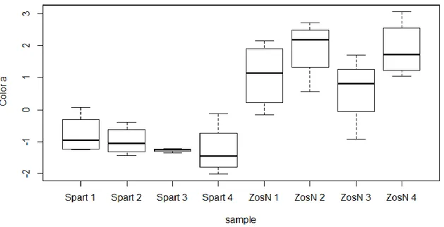
The grain size results are presented in Table 2.I in Annex 2. The textural composition of the samples varies between 5 and 25 % wv of clay (Fig. 3.1), 1 and 16 % wv of silt and 7 and 88 % wv of sand. The grain size of samples after removing the organic matter range 17.80 – 126.70 µm, with an average of 56 µm whereas the grain size of samples with organic matter range 21.34 – 1007.30 µm, with an average of 69.47 µm. The coarser sediment is found in station 1 for Z. noltii environment, whereas the finest sediment is from station 4 also in Z. noltii environment. Thus a progressive grain size diminution from station 1 to station 4 was observed, as well as a higher variability in Z. noltii than S. maritima. It is important to note that this gradient is mainly observed in the granulometry made on samples after removing the organic matter.
Figure 3.1: Percentage of clay size particles with no organic matter (% dw, Clay Mineral) in function of sampling station for each species.
Results
22
In a similar manner as seen for the Clay content from the sediment without organic matter (“Mineral Clay”), the fine/coarse ratio (Fig. 3.2) shows the same observed trend from station 1 to 4 with ratios varying from 1 to 6, but this time in both environments.
Figure 3.2: Percentage Fine/Coarse in function of sampling station for each species.
This similarity in trends can be verified in the high correlations observed between the two variables, being higher for Z .noltii than S. maritima with a value of 88% of correlation (Fig. 3.3), compared with a value of 44 % for S. maritima (Fig. 3.4).
Figure 3.3: Rplot correlations between the clay content from the sediment without organic matter (“Mineral Clay”) and fine/coarse ratio in Z. noltii.
Results
23
Figure 3.4: Rplot correlations between the Clay content from the sediment without organic matter (“Mineral Clay”) and fine/coarse ratio in S. maritima.
When observing the `particle size distribution classification’ (PSDC) of sediment type based on the proportions of sand, silt and clay, which are plotted as a ternary diagram in Fig. 3.5, the classification correspond with the progressive grainsize diminution in Z. noltii, environment from station 1, with a high percentage of sand, to station 4, with a higher percentage of silt Fig. 3.5 (A), whereas S. maritima environment shows a smaller gradient, being able to group the stations 1 and 2 on one hand and 3 and 4 on the other (Fig. 3.5 (B).
Nevertheless, both environments are characterized by silty sand in station 1 and silt in station 4, even though S. maritima environments show slightly coarser sediment due to a higher content of silt in relation to the clay content.
Results
24
Figure 3.5: Grain size ternary diagram for sediment classification (Folk 1954) showing the classification schemes for Z. noltii (A) and S. maritima (B) based on the relative percentages of sand, silt and clay. The numbers inside of the blue circle indicate the stations.
(A)
Results
25
3.1.2. Diffuse Reflectance Spectroscopy for color determination.
Color results obtained in each of the treatments are summarized in Table 2.V in the Annex 2. L* measured in the samples with organic matter (L*) has a range of variation between 47.08 and 66.40, whereas L* measured in samples after removing the organic matter (L*.no.OM) varies between 0 and 20.50. Similarly, a* varies from -2 to 3.06 and a*.no.OM between 0 and 47.08 whereas b* ranges from 16.28 to 33.70 and b* no.OM from 0 to 99.72 (see table2.V in annex 2).
These results clearly show differences between samples containing organic matter and samples after removal of organic matter.
The results of the analyzed samples that contained organic matter, show that the a* color present significant difference (ANOVA, p<0.001) between the Z. noltii environment and S. maritima environment. The highest values are found in Z. noltii environment and the smallest values in S. maritima (Fig.3.6). In the case of S. maritima environments values are below 0, thus colors with a green component, whereas for Z. noltii environments values are above 0, corresponding to a red component.
Results
26
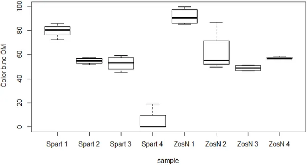
In the other hand b *(ANOVA, p >0.05) and L* (ANOVA, p>0.05) colors do not provide information for samples with organic matter (not shown here), nor does L* in samples after organic matter removal, showing no significant differences (ANOVA, p >0.05) by environments, i.e. there are no significant changes in these color components.
When observing the results of the analyzed samples after removal of the organic matter, both a*no.OM (ANOVA, p<0.001) (Fig.3.7) and b*no.OM (ANOVA, p<0.001) (Fig.3.8) colors show differences in function of the sampling station for each specie and between species. High values for both colors are registered in station 1 for S. maritima environment, whereas station 4 is characterized by smaller values in S. maritima environment, showing thus a progressive diminution of the values of both colors from station 1 to station 4.
Results
27
Results
28
3.1.3. Mineral identification.
With respect to the analysis of mineral composition, no significant differences in the sediments are found neither between types of environment or between stations (Fig 3.9). All the samples had a similar mineral composition (Table 3.1). However, some samples have small amounts (< 5%) of plagioclase, feldspars or siderite. Furthermore, it is important to note that the biggest difference in the mineral composition is in the percentages between quartz and clay minerals. The quartz percentage is higher in the station nearer to the main channel than the more remote station, the opposite occurs for clay minerals, their percentage increased from station 1 to station 4. With respect to the difference between biological communities, generally the mineralogical composition for Z. noltii is more variable and complex than for S. maritima.
Table 3.1: Mineral composition (%) for each station in function of sampling station for each species.
Sp1 Sp2 Sp3 Sp4 Zn1 Zn2 Zn3 Zn4 Mineral % % % % % % % % Pyrite 2.4 Goetite Hematite Magnesite Siderite 4.2 4.2 3.2 3.4 7.3 8.4 Dolomite Ankerite Calcite 1.4 2.6 2.1 Plagioclase 3.7 2.4 5 3.3 3.5 3.7 Feldspar K 3.4 2.8 3.8 3.5 3 2.2 Quartz 80 82 59 62 95 85 69 48 Aragonite Anhydrite 1.6 Cristobalite Phylosilicates 15 10 33 32 19 14 37 Gypsum 2.8 2.8
Results
29
Figure 3.9: Pattern of X-ray diffractometer for all the samples.
3.2. Geochemical Analysis.
3.2.1. Determination of Water, Organic matter and carbonate contents by Lost of Ignition.
The results of water, organic matter and carbonate contents are presented in Table 3.I in Annex 3. The water contents have an average value of 46.12 % ww, with a minimum of 22.68 % ww for station 1 in the Z. noltii (Zn1c) environment and a maximum of 57.80 % ww for the station 4 in environment of Z. noltii (Zn4d).
5 10 15 20 25 30 35 40 45 50 55 60 65 2Theta (°) 0 100 400 900 1600 2500 In te n s it y ( c o u n ts )
Results
30
The existence of a difference in water content is observed between the two environments (S. maritima and Z. noltii) (ANOVA, p<0.001), S. maritima presents an average off 11% ww more than Z. noltii. In both environments, there are differences between stations (ANOVA, p<0.001), there is an increase in water content throughout stations. Furthermore, it is possible to note also stabilization in the stations more distant from the main channel. For each environment, the smallest percentage of water content is found in station 1, whereas the highest percentage is from station 4 in Z. noltii environment, showing thus a progressive increase from station 1 to station 4(Fig.3.10).
Figure 3.10: Water content (% ww) in function of sampling station for each species.
Regarding organic matter content, data show an average of 7.9 % dw, with a minimum and a maximum of 1.85 % dw and 11.92 % dw for stations 1 from Z. noltii (Zn1c) and 2 from S. maritima (Sp2a) respectively.
When observing Figure 3.11, it is possible to observe differences (ANOVA, p<0.001) in the content of organic matter between both environments. Hence, S. maritima environments present higher average of 9.87 % dw than for Z.noltii with an average of 5.93 % dw of organic matter. In S. maritima, the percentage of organic matter does not have significant variations between stations, but it is important to note the existence of
Results
31
differences between station 1 and the other ones. In Z. noltii environments, a progressive gradient is observed again with the percentage of organic matter increasing from station 1 to station 4.
Figure 3.11: Organic matter content (% dw) in function of sampling station for each species.
In relation to carbonate content, its average value is 2.54 % dw, with a minimum of 0.62 % dw for station 3 in S. maritima (Sp3c) and, a maximum of 4.08 % dw for station 4 in Z. noltii (Zn4d).
Results
32
Figure 3.12: Carbonate content (% dw) in function of sampling station for each species.
As it can be observed in Figure 3.12, carbonates contents show significant differences (ANOVA, p<0.01) in Station 4 of Z. noltii environment with respect to other stations, whereas there is no significant difference (ANOVA, p>0.05) between the environments.
3.2.2. Determination of Elemental composition: OC, IC, ON, IN and C/N.
The Elemental composition results are presented in Table 3.II in Annex 3. This composition varies between 0.29 and 3.23 % dw, with an average value of 1.75 % dw of OC (organic carbon), 0.03 and 3.23 % dw, with an average value of 0.20 % dw of ON (organic nitrogen), 0.01 and 1.11 % dw with an average value of 0.53 % dw of IC (inorganic carbon) and -0 and 0.13 % dw, with an average value of 0.05 % dw of IN (inorganic nitrogen).
The highest organic carbon content is found in station 4 for Z. noltii environment (Zn4b), whereas the smallest percentage is from station 1 also in Z. noltii environment (Zn1b), showing thus a progressive increase of the organic carbon content from station 1 to station 4 as well as a higher variability in Z. noltii environments (Fig. 3.13). It is important to note that this same gradient is also observed in the result of the organic nitrogen content
Results
33
(Fig. 3.15), where the maximum value is found in station 4 for S. maritima and the minimum value is found in station 1 for Z. noltii (Zn1b and Zn1c). It is possible to observe differences (ANOVA, p<0.001) for both, organic carbon and organic nitrogen contents with respect to the different environments. The organic carbon content was almost double for S. maritima than Z. noltii, 2.25% dw and 1.24% dw, respectively. In the other hand, the organic nitrogen content was also double for S. maritima than Z. noltii, 0.27 % dw and 0.14 % dw.