UNIVERSIDADE DA BEIRA INTERIOR
Ciências Sociais e Humanas
ON THE RELATIONSHIP OF ENERGY AND CO2: THE
EFFECT OF FINANCIAL DEEP ON OIL PRODUCING
COUNTRIES
Mónica Alexandra Marques Lopes
Dissertation to obtain master degree in
Economics
(2
ndcycle of studies)
Adviser: Prof. Doutor José Alberto Serra Ferreira Rodrigues Fuinhas
ii
Acknowledgements
To my family, for the unconditional support provided during the academic journey and for reuniting all the social, economic and affective conditions.
To my friends, for delivering the necessary help in the harsh periods and for making everything easier through the good mood and companionship.
I would like to highlight the teacher’s role, especially Prof. Dr. Jose Alberto Fuinhas for accepting my guidance request and for the assistance provided during the essay elaboration.
Last but not least, enhance the active role of the people that interact with me until now.
iii
Resumo
O estudo analisa a relação de energia e CO2, evidenciando o efeito de profundidade financeira para um painel de 13 países produtores de petróleo. As emissões de CO2 são examinadas, tanto como um motor de crescimento, como variável explicada. O estudo utiliza o modelo Autoregressive Distributed Lag (ARDL), dados são anuais, cobrindo um período de 1970 a 2012. Os resultados mostram que as emissões de CO2 causam crescimento económico no curto prazo, e as emissões são causadas pelo crescimento, tanto no curto como no longo prazo. Rácio entre produção de petróleo e consumo de energia primária contribui para a redução das emissões de CO2, no curto e longo prazo, e contribui para o aumento do crescimento económico. A profundidade financeira contribui para o aumento das emissões de CO2 no curto prazo, já no crescimento contribui para a sua diminuição no curto e longo prazo. Inflação contribui para a diminuição do crescimento no longo prazo. Os resultados são consistentes em relação ao CO2 como sendo um motor de crescimento económico e vice-versa. Assim, os formuladores de políticas devem ter em conta que o crescimento económico pode levar a um aumento das emissões de CO2.
Palavras-chave
iv
Abstract
The relationship between energy and carbon dioxide emissions (CO2) and the financial depth was apprised within a panel of thirteen oil producing countries. The role of CO2 is analysed as economic growth driver and as explained variable. An Autoregressive Distributed Lag model with annual frequency data for the period from 1970 to 2012 was used. Our findings shown that CO2 promote economic growth in the short-run. The CO2 cause growth in long- and in short-run. The ratio between oil production and primary energy consumption impacts economic growth and the reduction of CO2 in long- and in short-run. The financial depth increases CO2 in short-run and depress economic growth both in long- and in short-run. The results for oil producing countries points to bidirectional causality between the CO2 and the economic growth. Therefore, policymakers of oil producing countries should be aware that economic growth may lead to an increase of CO2.
Keywords
v
Table of contents
1 – Introduction ... 1
2 – Literature Review... 2
3 – Data and Methodology ... 4
4 – Results ... 11
5 – Discussion ... 15
6 – Conclusion ... 17
vi
Tables List
Table 1 – Descriptive statistics and CSD Table 2 – Matrices of Correlations Table 3 – VIF statistics
Table 4 – Heterogeneous estimators, dynamic fixed effects, and Hausman tests Table 5 – Specification tests
Table 6 – Elasticities, semi-elasticities, impacts, and adjustment speed Table A – APPENDIX – Unit root tests
vii
List of Acronyms
CO2 ARDL EG FD GDP DCBS DCPS CSD VIF FE RE PMG MG OLSCarbon Dioxide Emissions Autoregressive Distributed Lag Economic Growth
Financial Depth
Gross Domestic Product
Domestic Credit provided by Banking Sector Domestic Credit provided by Private Sector Cross-Section Dependence
Variance Inflation Factor Fixed Effects
Random Effects Pooled Mean Group Mean Group
1
1. Introduction
The paper studies the relationship between energy and carbon dioxide emissions (CO2) and highlights the financial depth effect on oil producing countries. The role of CO2 is analysed as economic growth driver and as explained variable. To scrutinize the nexus, a panel data entry with thirteen countries and a time period between 1970 and 2012 was used. The inclusion of inflation fulfil a gap on this nexus. Indeed, this indicator can be used as a proxy of economic instability for the oil producing countries.
The oil production and consumption has an active role on the literature. In fact, more than understanding their impact on economic growth, we need to realize other effects in the energy– growth nexus. This nexus raises concerns related with the environment, namely pollution and CO2. The relationship between CO2 and energy consumption is positive (Saidi and Hammami, 2015). In special, the role of financial development should be better comprehended to supplant the current lack of consensus (e.g. Goldsmith, 1969; Minier, 2009; Sadorsky, 2010; Kaminsky and Reinhart, 1999; Deidda and Fattouh, 2002; Wachtel, 2003). This lack of consensus could be explained by the focus of research tends to be directed for the oil exporter countries (Fuinhas et al., 2015).
The main objective of this paper is to understand the relationship between energy and CO2, highlighting the financial depth effect. To capture these effects, variables such as CO2, Gross Domestic Product, Oil Consumption, Exports, Oil Rents, Production, International Crude Oil Prices, Inflation, and Financial Depth were used. The fact of analysing a long- time period allows dynamic relationships between variables and therefore, the Autoregressive Distributed Lag (ARDL) model comes out as the most suitable. An empirically supported multivariate panel was elaborated with the following specifications: (i) Group of oil producing countries with available data; (ii) A review of the ratio between oil production and primary energy consumption; and (iii) verify the impacts of the second oil shock. Following the procedure, the econometric techniques allows: (a) the evaluation of long- and short-run effects (b) to overpass the issue of the order of integration of variables. The used estimator allows to work with variables integrated I(0) and I(1); and (c) the usage of long- time span allow evaluate the co-integration or the long- memory (fractional co-integration) relationships among variables.
The rest of the paper is organized as follows: Section 2 review of the literature. Section 3 describes data and methodology. Section 4 is centred on the results. In section 5, the results are discussed. Section 6 concludes.
2
2. Literature Review
The analysis of the relationship between energy and CO2 highlighting the effect of the Financial Depth and Inflation is largely a new approach given that the topic is rarely addressed. By the reverse, growth-energy nexus is well known study area. A literature survey on energy-growth nexus can be seen in Omri (2014) and Menegaki (2013).
The causal relationship between energy and growth suggests the incorporation of environmental issues and CO2. A literature survey on CO2-energy-growth nexus can be seen in Omri (2013). Furthermore, financial development associated with the growth-energy nexus is also featured at the literature. Financial depth can enhance economic growth and affect the demand for energy (Sadorsky, 2010). The empirical results reveal a positive and significant relationship between financial development and energy. This phenomenon occur when financial development is measured by the deposit money bank assets to GDP, financial system deposits to GDP, or liquid liabilities to GDP (Sadorsky, 2011). Following Karanfil (2009), Dan and Lijun (2009) examined the effect of financial development on primary energy use in Guangdong, China. They found unidirectional causality from energy use to financial development. The concern with the environment is reported in some studies, namely in the causality field. A literature survey on energy consumption, financial development, and economic growth and CO2 emission can be seen in Ziaei (2015).
Due to the complex relationship of causalities and despite of the huge amount of studies in this area, the consensus among authors was far from reached. In an empirical overview, there are five possible occurrences: (1) Growth hypothesis – energy as a positive effect on growth; (2) Neutral hypothesis – absence of causality; (3) Conservation hypothesis – unidirectional causality from growth to energy; (4) Feedback hypothesis – bidirectional causality between growth and energy; (5) Resource curse hypothesis – “negative” energy produces growth.
The resource curse hypothesis is suggested in the literature to analyse the causality relationships between energy and growth. This phenomenon may be described as an economic constraint to oil producer’s countries. Indeed, these countries expect to receive economic and social benefits from the wealth, generated by encouraging the local and national economy or indirectly by increasing tax revenues, as result of government involvement (Costa e Santos, 2013).
In the analysis of CO2 embodying the nexus growth-energy and oil producing countries development, there are two decisions that must be done: (1) what is the most relevant energy variable to explain CO2?; and (2) with oil production, what is the most suitable ratio to explain the relationship between energy-growth-development and CO2? To answer to the first question, following seminal literature the oil consumption is the one that produce most appropriate results. Moreover, primary energy consumption and the decomposition of oil primary energy consumption in other power sources can also be used. Decomposing a variable allows a better comprehension of the main role of oil consumption in primary energy context (Fuinhas et al., 2015). The same authors highlight the importance of integrating oil consumption and productions variables as well as oil prices and international oil prices. It is expected that oil producer countries reveal some
3 idiosyncrasies, i.e. the existence of price volatility due to special circumstances, derived of the high correlation between fossil fuels and CO2.
The nexus complexity may be harmed by the endogenous resources availability. That availability can be controlled through the computation. A literature gap can be verified with the lack of inflation on the group of financial variables. Furthermore, inflation may exert a positive or a negative impact on growth. The positive effect can occur due to the excess of demand and inciting a tireless rise of prices, and the negative effect stems of measuring economic instability, suggesting a possible economic volatility. With the oil producer countries, a negative coefficient is expected. In fact, the inflation and the relationship between energy and CO2 is not in focus at the literature and therefore there is a limited understanding of this variable.
4
3. Data and methodology
For the analysis of the relationship between economic growth and CO2, was used a panel with annual frequency data from 1970 to 2012, for a group of oil producing countries, namely Saudi Arabia, Algeria, Australia, Denmark, Egypt, Ecuador, United States of America, India, Italy, Malaysia, Mexico, Peru and Trinidad and Tobago .These countries were chosen due to letting a continuous sample for the longest time span possible. The source of the raw annual data was the World Bank Data, for gross domestic product (GDP), exports of goods and services, oil rents, population, domestic credit provided by banking sector, domestic credit provided by private sector, and consumer price index; and the BP Statistical Review of World Energy, June 2014, for carbon dioxide emissions, oil consumption, oil production, primary energy consumption, and crude oil prices. The raw data variables used are: (i) GDP (constant local currency unit); (ii) exports of goods and services (% of GDP); (iii) oil rents (% of GDP); (iv) population (total of persons); (v) carbon dioxide emissions (million tonnes); (vi) oil consumption (million tonnes); (vii) oil production (million tonnes); (viii) primary energy consumption (million tonnes oil equivalent); (ix) crude oil prices (US dollars per barrel, 2013); (x) inflation (measured by first differences of logs of consumer price index); (xi) financial depth (% of GDP). The option of using a constant local currency unit allowed the influence of exchange rates to be circumvented. The econometric analysis was performed using Stata 13.1 and EViews 9 software.
The raw variables were transformed in: (a) CO2 emissions per capita (CO2PC); (b) Gross Domestic Product per capita (YPC); (c) Exports of goods and services per capita (XPC); (d) Oil rents
per capita (ORPC); (e) Oil consumption per capita (OCPC); (f) Ratio between oil production and
energy consumption (SE) - this ratio is used to control the heterogeneity and the oil production (Fuinhas et al., 2015), and can measure the importance of oil production in terms of primary energy; (g) Ratio between oil production and consumption (SO) – this ratio registers the progress made during a time period of the relative weight of oil production to oil consumption, and is used to control the heterogeneity of oil producers; (h) Oil prices (P) – defined as the international oil price, this variable is equal to all countries. (i) Inflation (INFL) – computed as the first differences of the natural logarithms of the consumer price index; (j) Financial Depth (PF) – computed as the aggregation of the Domestic Credit Provided by Banking Sector (DCPS) and the Domestic Credit Provided by Private Sector divided by the GDP.
The study follows two different approaches: (i) the first one evaluates the impact of CO2 as a source of economic growth with inflation as background; (ii) the second, using the same data, tries to capture the economic growth effect on CO2. Both approaches can be found at the literature. It is common to use Gross Domestic Product, measures of energy consumption, energy prices and traditional production factors. Occasionally, variables like exportations, CO2 per capita or urbanizations (e.g. Mohammadi and Parvaresh, 2014) or oil prices and production in scale (Fuinhas et al., 2015) or even financial development are used (Nili and Rastad, 2007). The inflation is rarely used in these approaches. This variable can have either coefficient signals, positive (as a
5 result of excess of demand causing a rise of production and prices) or negative (as a result of measuring economic instability).
The dynamical effects are expected due to the long span of time. Different behaviours in the long- and short-run are also expected. The computation of the variables was made through the UECM from the ARDL, introduced by Pesaran and Shin (1999). The ARDL estimator possesses all the necessary properties to generate consistent and efficient parameters. Moreover, the estimator can deal with variables with integration order I(0) and I(1) and work as a support to the standard errors. The variables used are expressed in Logarithms (L) and first differences (D). The first coefficients match to the elasticities and the seconds to the semi-elasticities.
The relationship between energy and CO2 will be tested with two different processes to capture the financial depth effect. First the growth model (YPC) evaluate the CO2 effect over the economic growth. Second, the CO2 model (CO2PC) assess the drivers of CO2. Severe attention must be paid to the individual coefficient interpretation. Indeed, with multivariate models all the independent variables are relevant and contribute to describe the dependent variable. The explanations provided should have in count the dynamical effects.
The used countries share some common characteristics like oil production. Like that, Cross Section Dependence (CSD) is expected. This phenomenon implies interdependence between the crosses due to the common shocks (Eberhardt, 2011). If countries react in the same way to shocks the existence of correlations is verified. This fact suggests the existence of common non-observable events. Taking this in account, Table 1 with the descriptive statistics, coefficients of variation and individual CSD test is presented.
6 Table 1
Descriptive statistics and CSD
Variables Descriptive statistics CSD
Obs Mean Std. Dev. Min. Max. CV CD-test Corr Abs (Corr) LCO2PC 559 -12.3393 1.21235 -14.788 -10.095 -0.0983 17.93*** 0.31 0.634 LYPC 559 9.8655 1.29406 7.02201 12.6021 0.13117 37.07*** 0.641 0.706 LEPC 559 -13.3529 1.1935 -15.963 -10.974 -0.0894 26.42*** 0.457 0.615 LOCPC 559 -14.0588 1.1426 -17.164 -12.281 -0.0813 -1.34 -0.023 0.643 LOEPC 559 -14.2418 1.42846 -17.405 -11.061 -0.1003 46.74*** 0.809 0.809 LXPC 558 8.41733 1.56812 5.02178 12.7704 0.1863 37.16*** 0.643 0.694 SE 559 1.49718 2.47482 0 18.1184 1.65299 8.49*** 0.15 0.523 SO 559 2.6922 3.499 0 23.7244 1.29968 4.30*** 0.073 0.42 LORPC 557 6.25801 2.0772 0.12944 10.8107 0.33193 35.76*** 0.628 0.643 LP 559 3.76559 0.60456 2.37893 4.74686 0.16055 56.39*** 1 1 LINFL 547 1.80612 1.08989 -2.8623 6.07035 0.60344 21.30*** 0.376 0.38 PF 559 1.18E-09 1.95E-09 1.67E-11 1.09E-08 1.65254 4.12*** 0.067 0.452 DLCO2PC 546 0.01988 0.0612 -0.3042 0.34734 3.07883 3.81*** 0.067 0.165 DLYPC 546 0.01972 0.04012 -0.1812 0.21532 2.03422 5.93*** 0.104 0.187 DLEPC 546 0.0218 0.05657 -0.2947 0.31923 2.59447 4.63*** 0.081 0.169 DLOCPC 546 0.00876 0.09277 -0.9672 0.59167 10.5943 3.19*** 0.056 0.156 DLOECP 546 0.04126 0.09966 -0.6286 0.5448 2.41544 4.60*** 0.08 0.153 DLXPC 545 0.03771 0.18545 -2.1872 1.94233 4.91845 12.21*** 0.213 0.296 DSE 546 -0.03919 0.51879 -4.4162 4.56445 -13.239 -0.89 -0.019 0.178 DSO 546 -0.0405 0.83563 -7.5098 6.84536 -20.63 -0.14 -0.006 0.163 DLORPC 544 0.077 0.39113 -1.1777 3.06568 5.07939 40.35*** 0.732 0.732 DLP 546 0.05598 0.29864 -0.6655 1.15456 5.33472 54.97*** 1 1 DLINFL 528 0.00567 0.59625 -3.0568 3.20465 105.26 10.54*** 0.193 0.215 DPF 559 1.18E-09 1.95E-09 1.67E-11 1.09E-08 1.65254 3.55*** 0.066 0.131 Notes: CV denotes coefficient of variations, i.e. the ratio of the standard deviation to the mean; CD test has N(0,1)
distribution, under the H0: cross-section independence. *** denotes significant at 1% level. The Stata command xtcd was used to compute CSD tests.
Through the Table 1 the highly dependence of the variables can be checked. With significance values of 1%, this shows that an introduced shock may affects in the same way all the countries. The CO2 was increased less than the economic growth. Moreover, CSD is not present in the variables LOCPC, SE and SO. This fact suggests that the countries react in different ways to the oil consumption and to de ratios oil production to oil consumption or primary energy consumption.
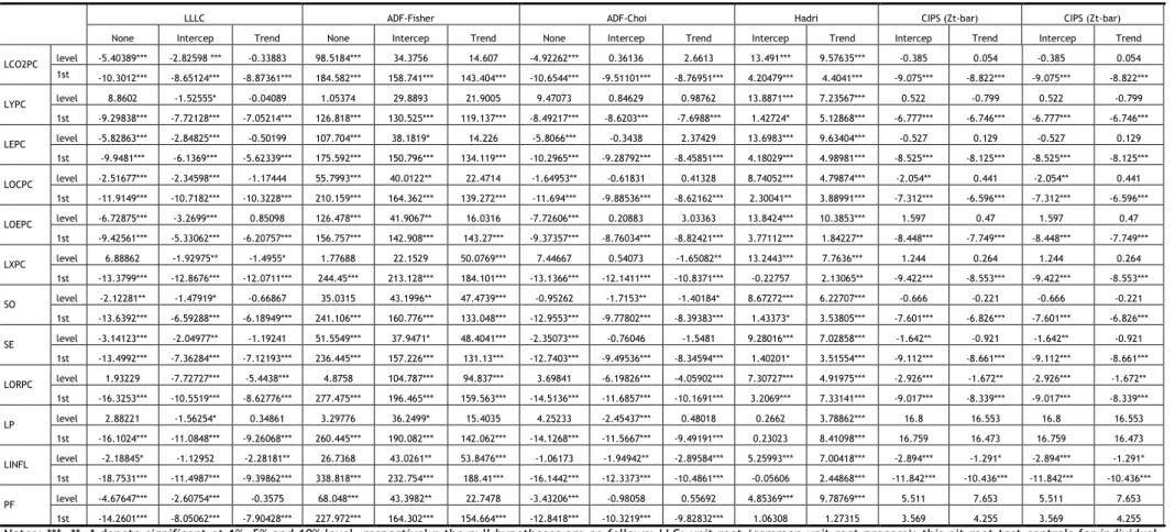
The unit root tests of first and second generation were applied to verify the integration order of the variables, i.e. I(0) and I(1). The first generation tests used were Levin Lin e Chu (2002) (LLC), ADF-Fisher (Maddala e Wu, 1999), ADF-Choi (Choi, 2001), while the second generation test was CIPS (Pesaran, 2007). This test has the advantage of being robust for heterogeneity and relax the cross-sectional independence assumption. After computing the tests, it was confirmed that the variables are integrated I(0) and I(1). The absence of I(2) variables allows consistent estimations for the dynamical estimators. The results can be checked at Annex A.
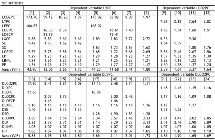
Another issue referred at the literature is the collinearity, i.e. the correlation between variables. Correlated variables mean that the independent variables explain in the same way the dependent variable. The correlation coefficients can be viewed at Table 2 and VIF statistics, to test
7 the multicollinearity, at Table 3. The VIF statistics were computed in level and first differences for both models, YPC and CO2PC.
Table2
Matrices of correlations
LCO2PC LYPC LEPC LOCPC LOECP LXCP SE SO LORPC LP LINFL PF
LCO2PC 1 LYPC 0.6711 1 LEPC 0.9964 0.6417 1 LOCPC 0.9218 0.5615 0.9237 1 LOECP 0.9297 0.6453 0.9329 0.7501 1 LXCP 0.685 0.9007 0.6692 0.603 0.6324 1 SE -0.0535 -0.1061 -0.0521 0.0639 -0.2064 0.0386 1 SO 0.0109 -0.082 0.0237 0.0118 -0.0407 0.0961 0.8993 1 LORPC 0.3254 0.4123 0.3292 0.2709 0.3147 0.5606 0.4276 0.5247 1 LP 0.0824 0.0871 0.0884 0.0443 0.1308 0.1512 -0.06 -0.0452 0.3171 1 LINFL -0.3499 -0.2637 -0.339 -0.2838 -0.369 -0.3293 0.0469 0.0196 -0.047 0.0809 1 PF 0.1112 -0.0497 0.1369 -0.0014 0.162 0.1377 0.0344 0.2684 0.2864 -0.0744 0.0171 1
DLCO2PC DLYPC DLEPC DLOCPC DLOECP DLXPC DSE DSO DLORPC DLP DLINFL DPF
DLCO2PC 1 DLYPC 0.3569 1 DLEPC 0.9703 0.3501 1 DLOCPC 0.6422 0.2548 0.5918 1 DLOECP 0.3948 0.1367 0.5227 -0.0208 1 DLXPC 0.0375 0.2034 0.033 -0.0239 0.0053 1 DSE -0.2331 0.4059 -0.2613 -0.132 -0.1939 0.2154 1 DSO -0.2809 0.3104 -0.2661 -0.5573 -0.0262 0.1929 0.7969 1 DLORPC 0.0831 0.1988 0.0818 0.0481 0.0959 0.3489 0.2302 0.1869 1 DLP 0.0956 0.1936 0.0844 0.0702 0.0376 0.2557 -0.017 -0.0206 0.8037 1 DLINFL -0.0254 0.1195 -0.0154 -0.0281 0.0258 0.1242 0.1724 0.1463 0.1929 0.1821 1 DPF -0.0436 -0.2364 -0.0293 -0.117 0.0432 -0.0231 -0.061 0.0189 -0.1523 -0.2027 -0.0654 1
Following these tests the model specifications are presented, namely the growth model in level (Eq. 1) and in first differences (Eq. 2), where LENPC represents the combination of three variables: LEPC, LOCPC and LOEPC; Furthermore, SOP embodies two variables: SE and SO.
) , , , , , , 2 ( it it it it it it it
it f LCO PC LENPC SOP LORPC LP LINFL PF
LYPC (1) ) , , , , , , , 2 ( it it it it it it it it
it f DLCO PC DLENPC DLXPC DSOP DLORPC DLP DLINFL DPF
DLYPC (2)
The specification of CO2 model in level (Eq. 3) and in first differences (Eq. 4) is exhibited next: ) , , , , , , , (
2PCit f LYPCit LENPCit LXPCit SOPit LORPCit LPit LINFLit PFit
LCO (3) ) , , , , , , , (
2PCit f DLYPCit DLENPCit DLXPCit DSOPit DLORPCit DLPit DLINFLit DPFit
8 Scrolling down from Table 2 to Table 3, some unwished coefficients can be observed. For the matrix table, a correlation coefficient that overpasses 0.8 reveals potential multicollinearity and may lead to some concerns. The energy variables (LEPC, LOCPC, and LOEPC) are strongly correlated with CO2 (LCO2PC) and exports of goods and services (LXPC) are strongly correlated with GDP (LYPC). To overcome this problem, the variables LEPC and LOEPC from the growth model and LXPC from the CO2 will be removed of estimations.
Table 3 VIF statistics
Dependent variable LYPC Dependent variable LCO2PC [1] [2] [3] [4] [5] [6] [7] [8] [9] [10] [11] [12] LCO2PC 173.70 59.12 10.23 1.97 175.02 58.02 9.09 1.97 LYPC 7.86 2.12 7.64 2.02 LEPC 166.87 168.02 LOCPC 16.33 8.39 16.61 7.40 1.63 1.54 1.60 1.51 LOECP 21.79 19.41 LXCP 2.88 2.83 2.69 2.69 2.89 2.83 2.72 2.72 9.33 9.30 SE 1.42 1.93 1.62 1.42 1.64 1.59 SO 1.63 1.73 1.63 1.62 1.80 1.76 LORPC 2.52 2.75 2.58 2.51 2.65 2.72 2.65 2.65 2.56 2.46 2.67 2.56 LP 1.29 1.28 1.28 1.28 1.29 1.28 1.28 1.27 1.37 1.32 1.35 1.30 LINFL 1.21 1.26 1.23 1.21 1.21 1.25 1.23 1.21 1.22 1.13 1.22 1.13 PF 1.31 1.26 1.25 1.19 1.29 1.27 1.27 1.17 1.50 1.28 1.37 1.20 Mean (VIF) 43.90 12.06 3.66 1.75 44.25 11.68 3.41 1.80 3.39 1.64 3.37 1.64 Dependent variable DLYPC Dependent variable DLCO2PC [13] [14] [15] [16] [17] [18] [19] [20] [21] [22] [23] [24] DLCO2PC 17.30 2.41 1.81 1.09 17.15 2.48 1.74 1.11 DLYPC 1.48 1.46 1.19 1.16 DLEPC 17.66 16.98 DLOCPC 2.03 1.73 3.00 2.48 1.17 1.16 1.09 1.08 DLOECP 1.45 1.46 DLXPC 1.16 1.16 1.16 1.16 1.16 1.16 1.16 1.16 1.17 1.17 DSE 1.40 1.39 1.35 1.35 1.59 1.58 DSO 1.28 1.90 1.83 1.28 DLORPC 3.60 3.64 3.54 3.54 3.34 3.57 3.46 3.33 3.61 3.47 3.02 2.85 DLP 3.36 3.37 3.31 3.31 3.14 3.29 3.23 3.13 3.46 3.46 2.90 2.89 DLINFL 1.08 1.07 1.07 1.07 1.07 1.07 1.07 1.06 1.07 1.07 1.06 1.05 DPF 1.06 1.07 1.07 1.06 1.05 1.07 1.07 1.05 1.10 1.10 1.10 1.10 Mean (VIF) 5.83 1.96 1.88 1.80 5.65 2.11 2.01 1.73 1.83 1.90 1.65 1.69 The estimations with the best results will be used, therefore the ARDL specifications for the growth model (Eq. 5) is shown:
k j it j it ij k j j it ij k j j it ij k j j it ij j it k j ij k j k j k j ij j it ij j it ij t i i PF LINFL LP LORPC LXPC LOCPC PC LCO LYPC TREND LYPC 0 1 18 0 18 0 17 0 16 0 14 1 0 0 13 12 11 1 1 2 (5)where α1i denotes the intercept; δ1i, β1kij, k=1,…,m, the estimated parameters, and ε1i the error
term.
The Eq. 5 can be rewritten in UECM form (Eq. 6) with the proposal of decomposing the dynamic relationships in short- and long-run as follows:
9 it it i it i it i it i it i it i it i k j k j it i it i j it ij j it ij k j k j k j j it ij k j j it ij j it ij j it ij k j k j j it ij j it ij t i i PF LINFL LP LORPC SE LXPC LOCPC PC LCO LYPC DPF DLINFL DLP DLORPC DSE DLXPC PC DLCO DLYPC TREND DLYPC 2 1 29 1 28 1 27 1 26 1 25 1 24 1 23 0 0 1 22 1 21 29 28 0 0 0 27 0 26 25 24 1 0 22 21 2 2 2 2
(6)where α2i denotes the intercept; δ2i, β2kij, k=1,…,m to the estimated parameters; and ε2i to the error
term. The ARDL specification for CO2 model (Eq. 7) is shown next:
k j it j it ij j it k j ij k j j it ij k j j it ij k j k j j it ij j it ij k j k j j it ij j it ij t i i it PF LINFL LP LORPC SE LOCPC LYPC PC LCO TREND PC LCO 0 3 38 0 37 0 36 0 35 0 0 34 33 1 0 32 31 3 3 2 2 (7)where α3i denotes the intercept; δ3i, β3kij, k=1,…,m, the estimated parameters; and ε3i the error
term.
This equation 7 can be rewritten in UECM form (Eq. 8) with the proposal of decomposing the dynamic relationships in short- and long-run as follows:
it it i it i it i it i it i it i k j k j it i it i j it ij j it ij k j j it ij k j j it ij k j k j j it ij j it ij k j j it ij k j j it ij t i i it PF LINFL LP LORPC SE LOCPC LYPC PC LCO DPF DLINFL DLP DLORPC DSE DLOCPC DLYPC PC DLCO TREND PC DLCO 4 1 48 1 47 1 46 1 45 1 44 1 43 0 0 1 42 1 41 48 47 0 46 0 45 0 0 44 43 0 42 1 41 4 4 2 2 2
(8)The presence of individual effects ought to be tested against random effects. For the random effects (RE) growth model, in Eq. (9), the error assumes the form ε5it=µ5i +ω5it, where µ5i
denotes the N-1 country-specific effects and ω5it are the independent and identically distributed
errors. In conformity, Eq. (6) is converted in Eq. (9):
it i it i it i it i it i it i it i it i it i k j k j k j it i j it ij j it ij j it ij k j k j j it ij j it ij k j k j j it ij j it ij k j k j j it ij j it ij t i it PF LINFL LP LORPC SE LXPC LOCPC PC LCO LYPC DPF DLINFL DLP DLORPC DSE DLXPC DLOCPC PC DLCO DLYPC TREND DLYPC 5 5 1 59 1 58 1 57 1 56 1 55 1 54 1 53 1 52 0 0 0 1 51 59 58 57 0 0 56 55 0 0 54 53 1 0 52 51 6 5 2 2
(9)where α5 denotes the intercept; δ5i, β5kij, k=1,…,m, e γ5im the estimated parameters; and µ5i +ω5it
the error term. For the random effects (RE) CO2 model, in Eq. (10), the error assumes the form ε6it=µ6i+ω6it, where µ6i denotes the N-1 country-specific effects and ω6it are the independent and
10 it i it i it i it i it i it i it i k j k j it i it i j it ij j it ij k j k j j it ij j it ij k j k j j it ij j it ij k j k j j it ij j it ij t i it PF LINFL LP LORPC SE LYPC LOCPC PC LCO DPF DLINFL DLP DLORPC DSE DLOPC DLYPC DLOCPC TREND PC DLCO 6 6 1 68 1 67 1 66 1 65 1 64 1 63 0 0 1 62 1 61 68 67 0 0 66 65 0 0 64 63 1 0 62 61 6 6 2 2
(10)where α6 represents the constant term; δ6i, β6kij, k=1,…,m, and γ5im are the estimated parameters;
and µ6i +ω6it corresponds for the error term.
The following step was attesting the model specifications trough the Hausman test. This test faces fixed effects (FE) with (RE). According to the Hausman test, the null hypothesis represents RE model while the alternative hypothesis indicates FE model. The FE model reveals evidence of individual correlation between countries and removes all the invariant characteristics. The Hausman test selected the FE as the most suitable estimator. Indeed this result establish the necessity of computing another tests, namely to apprise the heterogeneity. For a dynamic approach, the heterogeneity may assume two shapes: (i) short- and long-run; and (ii) short-run. To deal with this, the estimators Mean Group (MG) and (PMG) could be applied. These estimators require a large number of observations (N) and time (T) (Blackburne III and Frank, 2007). The MG model is the most flexible, by enabling the heterogeneity of the coefficients between countries. This model is effective when long- and short-run estimations are made, but ineffective against homogeneity (Pesaran et al., 1999). This model needs a long span of time and a large number of countries, 20 to 30 countries (Ciarlone, 2011). The PMG allows the existence of heterogeneity in the coefficients of short-run and homogeneity in the coefficients of long-run. If the presence of homogeneity in the coefficients of long-run is confirmed, the PMG model will be chosen as the most suitable.
11
4. Results
The exhaustive control of the integration order of the variables is being conclusive as was shown at Annex A. As explained before, the econometric techniques must be suitable to deal with variables integrated as I(0) and I(1). To assess the presence of heterogeneity, the MG and PMG were carefully exanimated and tested against the dynamic FE estimator.
The MG, PMG and FE model estimations as the results of the Hausman test are provided at Table 4. The variables without any significance were removed from the model. Moreover, trend and LORPC from the growth model, likewise the variables LOCPC, LORPC, LP and LINFL from CO2 model are not statistically significant.
Table 4
Heterogeneous estimators, dynamic fixed effects, and Hausman tests Growth model (Dependent variable DLYPC)
MG(I) PMG(II) FE(III)
Constant 3.6460*** 1.4138*** 0.8398*** LOCPC 0.5563*** 0.1622*** 0.2108*** LXCP 0.2822*** 0.1923*** 0.3873*** SO 0.6189 0.0183* 0.0626*** LORPC 0.0624 0.0334*** -0.0249 LINFL -0.0618** -0.0763*** -0.0467**
PF -2.10E+07 -5.3E+07*** -7.5E+07***
ECM -0.2484*** -0.1316*** -0.0854*** Trend 0.0020* 0.0006* 0.0003 DLCO2PC 0.2167*** 0.1663* 0.1397*** DLOCPC 0.1514** 0.1815* 0.1988*** DLXPC 0.0363** 0.0389*** 0.0257*** DSO 0.0850*** 0.0476*** 0.0340*** DLORPC -0.0168 -0.0289** -0.0253*** DLP 0.0261** 0.0384*** 0.0332***
DPF -2.30E+07 -1.7E+07* -2.4E+07***
Models MG vs PMG PMG vs FE MG vs FE
Hausman tests
Chi2(2)=-31,05 Chi2(2)=0,00 Chi2(2)=0,00 CO2 model (Dependent variable DLCO2PC)
MG(I) PMG(II) FE(III)
Constant -4.7485*** -1.6993*** -0.8776***
LYPC 0.1695 0.3973*** 1.5031**
LOCPC 0.3612*** 0.4338*** -0.4031
12 LORPC 0.0588 0.1537*** 0.0532 LP -0.0268 -0.1322*** 0.0899 LINFL -0.0037 -0.0254*** -0.0598 ECM -0.4411*** -0.1582*** -0.0272** Trend 0.0028 -0.0001 -0.0008** DLYPC 0.3234*** 0.2974*** 0.6315*** DLOCPC 0.4641*** 0.5096*** 0.3025*** DSE -0.2525*** -0.3060*** -0.0456*** DLORPC 0.0660*** 0.0546*** 0.0280*** DLP -0.0614*** -0.0499*** -0.0283**
DPF 1.3E+07*** 7.4E+06*** 1.8E+07***
Models MG vs PMG PMG vs FE MG vs FE
Hausman tests
Chi2(1)= n.
a. Chi2(1)=0,00 Chi2(1)=0,00 Notes: ***, **, * denote significant at 1%, 5% and 10 % level, respectively; Hausman results (with the options sigmamore, alleqs, and constant) for H0: difference in coefficients not systematic; ECM denotes error correction mechanism; the long-run parameters are computed elasticities; the Stata command xtpmg was used; n. a. denote not available.
The Hausman test of MG vs PMG for the growth model presents a negative coefficient. Indeed, the negative x2 from Hausman test although uncommon (see Dincecco, 2010) emphasizes
the rejection of the first estimator (Hausman, 1984; Fuinhas et al., 2015). From Table 4 we can observe that the FE estimator is the most suitable, i.e. there is homogeneity for both models in the panel data entry. These results sustain that oil producing countries share same coefficients and can be treated in the same way.
To reinforce the FE parameter significance, several tests were made to identify the existence of econometric violations, namely heteroskedasticity, correlations, autocorrelations and CSD. The Wald test was used to control the heteroskedasticity of the residuals. Next he Pesaran test analyses the presence of contemporaneous relationships between crosses. The null hypothesis specifies that the residuals are not correlated and follow a normal distribution. The Breusch-Pagan Lagrangian Multiplier was applied to test the cross sectional Independence and verify the correlation between errors. At last, the Wooldridge test assesses the presence of autocorrelation of first order. The results are revealed at Table 5.
13 Table 5
Specification tests
Tests Growth model CO2 model
Statistics
Modified Wald chi2(13)= 383.27*** chi2(13)= 1808.14***
Pesarant -1577 0.569
Breusch-Pagan LM n. a. n. a.
Wooldrige F(1,12) = 105.952*** F(1,12) = 40.842***
Note: *** denotes significant at 1% level; results for H0 of Hausman test (with the option sigmamore) : difference in coefficients not systematic; results for H0 of Modified Wald test: sigma(i)^2 = sigma^2 for all I; results for H0 of Pesaran and: residuals are not correlated; results for H0 of Wooldrige test: no first-order autocorrelation; n. a. denote not available.
The applied tests come out as appropriate and revealed the existence of heteroskedasticity, autocorrelation of first order and contemporaneous correlation. With these phenomena the elasticities and semi-elasticities, shocks and speed adjustments for both models are presented at the Table 6. The models were re-estimated and the significance of the variables was maintained. Furthermore, the elasticities of long-run have a different way of reading them. By the reverse, the short-run elasticities have a direct reading for having equal coefficients. To measure the long-run elasticities the ratio between the coefficient of each independent variable and the coefficient of the dependent variable (LYPC) for growth model and (LCO2PC) for CO2 model was made. Moreover, the variables had lag 1 and were multiplied by (-1). The results revealed Granger causal effects on both models (see Table 6).
14 Table 6
Elasticities, semi-elasticities, impacts, and adjustment speed
Growth model (Dep var. DLYPC) CO2 model (Dep var. DLCO2PC) Short-run DLCO2PC 0,1367*** DLYPC 0,6128*** DLOCPC 0,1973*** 0,3086*** DLXPC 0,0283*** DSE -0,0448*** DSO 0,0336*** DLORPC -0,0266*** 0,0303*** DLP 0,0343*** -0,0310*** DPF -2,44E^7*** 1,74E^7** Long-run LYPC 0,5725* LXCP 0,4565*** SE -0,1441* SO 0,0559*** LORPC -0,0247* LP 0,1237** LINFL -0,0558** PF -7,45E^7*** Speed of adjustment ECM -0,0805*** -0,0286*
Notes: ***, **, * denote significant at 1%, 5% and 10 % level, respectively; ECM denotes the coefficient of variable LYPC lagged once for the Growth model, and LCO2PC lagged once for the CO2 model; the long-run parameters are computed elasticities; and the Stata command xtscc with the options: fe, ase and lag(1) was used.
15
5. Discussion
The main objective of this study is highlighting the relationship between energy and CO2 among with financial development for a group of oil producer countries. Furthermore, 2 different views can be found through CO2: (1) First as a growth engine; and (2) as a dependent variable explained by his own drivers.
Preliminary tests revealed the presence of heteroskedasticity, CSD, residual correlation, first order autocorrelation and I(0) and I(1) of integration order. Moreover, the panel data entry used covers: (i) developed and developing countries; (ii) small and big oil producer countries; and (iii) to ensure a robust analysis, a large span of time was used. The dynamical panel data techniques are adequate to the study. Indeed, short- and long-run effects are detected, sustaining the former statement. The adjustment speeds are negative and statistically significant. The ECM term for the growth model is low (slightly over 8%, see table 8) while for the CO2 model is very low (under 3%). This fact suggests that a long span of time is needed when a shock is introduced. Likewise, the economic structure from the oil producer countries is weak and takes too much time to overpass possible shocks due to the lack of competitiveness.
The growth model reveals a high number of positive coefficients in the short- and long-run. Undeniably, some variables only present a short-run effect on growth, namely CO2 (CO2PC), oil consumption (OCPC) and International oil prices (P). In the main terms, the variables that have a higher impact on growth are the goods and services exportations (EXPC) at long-run and oil consumption (OCPC) at short-run. Additionally, a negative coefficient is verified at the oil rents (ORPC) and financial depth (PF) both on short- and long-run. The inflation has a negative coefficient too but only at long-run. Forward, a more detailed discussion will be provided.
At the CO2 model, variables like oil consumption (OCPC), oil rents (ORPC) and financial depth (PF) only enhances growth at the short-run. In this model, GDP (YPC) is the main propeller at short- and long-run. The relationship between oil production to consumption (SO) or primary energy consumption (SE) reveal explanation power at short- and long-run for both models. As result of this relationship, for growth have a positive impact while to CO2 as negative effect. This dissimilitude is expected. On the one hand, when oil production increases relatively to oil consumption this impacts positively on growth. On the other hand, the negative effect of the ratio of oil production to primary energy consumption indicates the phenomenon of concentration of wealth typical of economies that are resource abundant. Indeed, wealth concentration contributes to lower CO2 per
capita due to the specialization effect (Fuinhas et al., 2015).
Comparing both models expose interesting results. Indeed, oil prices (P) are highly significant at short- and long-run on both models. Furthermore, different signals are presented for the growth and CO2 models. A positive coefficient is revealed for the growth model and a negative one for the CO2 model. This phenomenon is consistent with the founded effect on oil rents (ORPC) and for financial depth (PF) with a negative effect on growth model and a positive effect on CO2 model. Therefore, when the oil extraction costs decrease, the local economic will all suffer the effect. The financial depth coefficient presents a negative impact on growth model and positive
16 impact on CO2 model. In fact, this phenomenon may occur due to the recent financial crisis, a weak banking sector, and low level of finance trough the banking sector. In a different perspective, a positive impact could be in the agenda if the financial sector presents a low level of development, like the high growth rate of credit market in economies in development, originating a GDP increase. At last, inflation revealed a negative coefficient in the long-run at the growth model due to her functions, i.e. capture the economic instability. This result was expectant attending to the group of countries selected. Therefore, the instability effect dominates the excess of demand. Hence, this outcome suggests the presence of an indirect weak growth hypothesis of the oil-growth nexus. Indeed, the analyses of the two models detect causality running from CO2 to growth, and causality running from oil consumption to CO2, in the short-run. The obtained results should be considered by the policymakers in order to apply better energy policies.
17
6. Conclusion
This paper analyses the relationship between energy and CO2, highlighting the role of financial depth and inflation. For this paper, annual frequency data from 1970 to 2012 for a group of thirteen oil producer countries was used. Additionally, CO2 are studied as a growth propellant and as explained variable.
The results contribute to the literature by providing a detailed explanation to the growth-CO2 nexus. Furthermore, the introduction of a new variable, namely inflation, revealed to be a good innovation. The financial institutions in oil producer countries are weak and financial sector is undeveloped. Other factor can be provided from the excess of financial system development. In the literature, excess of finance harms growth.
The consistence of the results suggest that the resources curse phenomenon should not be neglected and deserve be considered in the literature. In fact, most of the studies only use rents from exploration of endogenous resources. The results are consistent as the CO2 are an important growth driver and vice-versa. Moreover, the emissions cause economic growth on the short-run. A bi-directional relationship between CO2 and growth was shown. The ratio between oil production and primary energy consumption reduce CO2 at short- and long-run. At the growth model this ratio is a driver to growth. The oil consumption contributes for both growth and short-run CO2. Similar results are obtained with financial depth and oil rents. The inflations imply a decrease on growth at long-run while oil prices reduces CO2 in the short-run and enhance growth at short-run to. Both exportations and ratio between oil production and consumption increase the growth rate at short- and long-run. This phenomenon emphasizes that an increase in exports and surpluses promotes economic growth. Oil rents decrease the growth rate at short- and long-run, i.e. the resources curse could be considered as a blessing to these countries.
18
References
Blackburne III, E. F., Frank, M. W., (2007). Estimation of non-stationary heterogeneous panels. The
Stata Journal 7(2): 197-208.
Choi, I., (2001). Unit root tests for panel data. Journal of International Money and Finance, 20(1): 249-272.
Ciarlone, A., (2011). Housing wealth effect in emerging economies. Emerging Markets Review,
12(4): 399-417.
Costa, H. K. D. M., Santos, E. M. D., (2013). Institutional analysis and the “resource curse” in developing countries. Energy Policy, 63: 788-795.
Dan Y., Lijun Z., (2009). Financial development and energy consumption: an empirical research based on Guangdong Province. Paper presented at International Conference on Information Management, Innovation Management and Industrial Engineering, ICIII, 3: 102–105.
Deidda, L., Fattouh, B., (2002). Non-linearity between finance and growth. Economics Letters, 74(3): 339-345.
Dincecco, M., (2010). The political economy of fiscal prudence in historical perspective. Economics
and Politics, 22(1): 1-36.
Eberhardt, M., (2011). Panel time-series modeling: New tools for analyzing xt data. 2011 UK Stata Users Group meeting.
Fuinhas, J. A., Marques, A.C., Couto, A. P., (2015). Oil-Growth nexus in Oil Producing Countries: Macro Panel Evidence. International Journal of Energy Economics and Policy, 5(1): 148-163. Goldsmith R.W., (1969). Financial structure and development. New York: Yale University Press. Hausman, J., Mcfaden, D., (1984). Specification test for multinominal logit model. Econometrica,
52: 1219-1240.
Kaminsky, G.L., Reinhart, C.M., (1999). The twin crises: the causes of banking and balance-of payments problems. The American Economic Review, 89(03): 473-500.
Karanfil, F., (2009). How many times again will we examine the energy–income nexus using a limited range of traditional econometric tools? Energy Policy, 36: 3019–3025
19 Maddala, G.S., Wu, S., (1999). A comparative study of unit root tests with panel data a new simple test. Oxford Bulletin of Economics and Statistics, 61: 631-652.
Menegaki, A.N., (2013). Growth and energy nexus in Europe revisited: Evidence from a fixed effects political economy model. Energy Policy, 61: 881–887.
Minier, J., (2009). Opening a stock exchange. Journal of Development Economics, 90: 135–143. Mohammadi, H., Parvaresh, S., (2014). Energy consumption and output: Evidence from a panel of 14 oil-exporting countries, Energy Economics, 41: 41-46.
Nili, M., Rastad, M., (2007). Addressing the growth failure of the oil economies: The role of financial development. The Quaterly Review of Economics and Finance, 46: 726-740.
Omri, A., (2013). CO2 emissions, energy consumption and economic growth nexus in MENA countries: Evidence from simultaneous equations models. Energy Economics, 40: 657–664. Omri, A., (2014). An international literature survey on energy-economic growth nexus: Evidence from country-specific studies. Renewable and Sustainable Energy Reviews, 38: 951–959.
Pesaran, M.H., (2007). A simple panel unit root test in the presence of cross section dependence.
Journal of Applied Econometrics, 22(2): 265-312.
Pesaran, M.H., Shin, Y., Smith, R.P., (1999). Pooled Mean Group Estimation of Dynamic Heterogeneous Panels. Journal of American Statistical Association, 94(446): 621-634.
Sadorsky, P., (2010). The impact of financial development on energy consumption in emerging economies. Energy Policy, 38: 2528–2535.
Sadorsky, P., (2011). Financial development and energy consumption in Central and Eastern European frontier economies. Energy Policy, 39: 999 1006.
Saidi, K., Hammani, S., (2015). The impact of CO2 emissions and economic growth on energy consumption in 58 countries. Energy Reports, 1: 62-70.
Wachtel, P., (2003). How Much Do We Really Know about Growth and Finance? Economic Review,
88: 33-48.
Ziaei, S.M., (2015). Effects of financial development indicators on energy consumption and CO2 emissions of European, East Asian and Oceania countries. Renewable and Sustainable Energy
1 APPENDIX – A1
Table A Unit root tests
LLLC ADF-Fisher ADF-Choi Hadri CIPS (Zt-bar) CIPS (Zt-bar) None Intercep Trend None Intercep Trend None Intercep Trend Intercep Trend Intercep Trend Intercep Trend
LCO2PC level -5.40389*** -2.82598 *** -0.33883 98.5184*** 34.3756 14.607 -4.92262*** 0.36136 2.6613 13.491*** 9.57635*** -0.385 0.054 -0.385 0.054 1st -10.3012*** -8.65124*** -8.87361*** 184.582*** 158.741*** 143.404*** -10.6544*** -9.51101*** -8.76951*** 4.20479*** 4.4041*** -9.075*** -8.822*** -9.075*** -8.822*** LYPC level 8.8602 -1.52555* -0.04089 1.05374 29.8893 21.9005 9.47073 0.84629 0.98762 13.8871*** 7.23567*** 0.522 -0.799 0.522 -0.799 1st -9.29838*** -7.72128*** -7.05214*** 126.818*** 130.525*** 119.137*** -8.49217*** -8.6203*** -7.6988*** 1.42724* 5.12868*** -6.777*** -6.746*** -6.777*** -6.746*** LEPC level -5.82863*** -2.84825*** -0.50199 107.704*** 38.1819* 14.226 -5.8066*** -0.3438 2.37429 13.6983*** 9.63404*** -0.527 0.129 -0.527 0.129 1st -9.9481*** -6.1369*** -5.62339*** 175.592*** 150.796*** 134.119*** -10.2965*** -9.28792*** -8.45851*** 4.18029*** 4.98981*** -8.525*** -8.125*** -8.525*** -8.125*** LOCPC level -2.51677*** -2.34598*** -1.17444 55.7993*** 40.0122** 22.4714 -1.64953** -0.61831 0.41328 8.74052*** 4.79874*** -2.054** 0.441 -2.054** 0.441 1st -11.9149*** -10.7182*** -10.3228*** 210.159*** 164.362*** 139.272*** -11.694*** -9.88536*** -8.62162*** 2.30041** 3.88991*** -7.312*** -6.596*** -7.312*** -6.596*** LOEPC level -6.72875*** -3.2699*** 0.85098 126.478*** 41.9067** 16.0316 -7.72606*** 0.20883 3.03363 13.8424*** 10.3853*** 1.597 0.47 1.597 0.47 1st -9.42561*** -5.33062*** -6.20757*** 156.757*** 142.908*** 143.27*** -9.37357*** -8.76034*** -8.82421*** 3.77112*** 1.84227** -8.448*** -7.749*** -8.448*** -7.749*** LXPC level 6.88862 -1.92975** -1.4955* 1.77688 22.1529 50.0769*** 7.44667 0.54073 -1.65082** 13.2443*** 7.7636*** 1.244 0.264 1.244 0.264 1st -13.3799*** -12.8676*** -12.0711*** 244.45*** 213.128*** 184.101*** -13.1366*** -12.1411*** -10.8371*** -0.22757 2.13065** -9.422*** -8.553*** -9.422*** -8.553*** SO level -2.12281** -1.47919* -0.66867 35.0315 43.1996** 47.4739*** -0.95262 -1.7153** -1.40184* 8.67272*** 6.22707*** -0.666 -0.221 -0.666 -0.221 1st -13.6392*** -6.59288*** -6.18949*** 241.106*** 160.776*** 133.048*** -12.9553*** -9.77802*** -8.39383*** 1.43373* 3.53805*** -7.601*** -6.826*** -7.601*** -6.826*** SE level -3.14123*** -2.04977** -1.19241 51.5549*** 37.9471* 48.4041*** -2.35073*** -0.76046 -1.5481 9.28016*** 7.02858*** -1.642** -0.921 -1.642** -0.921 1st -13.4992*** -7.36284*** -7.12193*** 236.445*** 157.226*** 131.13*** -12.7403*** -9.49536*** -8.34594*** 1.40201* 3.51554*** -9.112*** -8.661*** -9.112*** -8.661*** LORPC level 1.93229 -7.72727*** -5.4438*** 4.8758 104.787*** 94.837*** 3.69841 -6.19826*** -4.05902*** 7.30727*** 4.91975*** -2.926*** -1.672** -2.926*** -1.672** 1st -16.3253*** -10.5519*** -8.62776*** 277.475*** 196.465*** 159.563*** -14.5136*** -11.6857*** -10.1691*** 3.2069*** 7.33141*** -9.017*** -8.339*** -9.017*** -8.339*** LP level 2.88221 -1.56254* 0.34861 3.29776 36.2499* 15.4035 4.25233 -2.45437*** 0.48018 0.2662 3.78862*** 16.8 16.553 16.8 16.553 1st -16.1024*** -11.0848*** -9.26068*** 260.445*** 190.082*** 142.062*** -14.1268*** -11.5667*** -9.49191*** 0.23023 8.41098*** 16.759 16.473 16.759 16.473 LINFL level -2.18845* -1.12952 -2.28181** 26.7368 43.0261** 53.8476*** -1.06173 -1.94942** -2.89584*** 5.25993*** 7.00418*** -2.894*** -1.291* -2.894*** -1.291* 1st -18.7531*** -11.4987*** -9.39862*** 338.818*** 232.754*** 188.41*** -16.1442*** -12.3373*** -10.4861*** -0.05606 2.44868*** -11.842*** -10.436*** -11.842*** -10.436*** PF level -4.67647*** -2.60754*** -0.3575 68.048*** 43.3982** 22.7478 -3.43206*** -0.98058 0.55692 4.85369*** 9.78769*** 5.511 7.653 5.511 7.653 1st -14.2601*** -8.05062*** -7.90428*** 227.972*** 164.302*** 154.664*** -12.8418*** -10.3219*** -9.82832*** 1.06308 1.27315 3.569 4.255 3.569 4.255
Notes: ***, **, * denote significant at 1%, 5% and 10% level, respectively; the null hypotheses are as follows: LLC: unit root (common unit root process); this nit root test controls for individual effects, individual linear trends, has a lag length 1, and Newey-West automatic bandwidth selection and Barttlett kernel; ADF-Fisher and ADF-Choi: unit root (individual unit root process); this unit root test controls for individual effects, individual linear trends, has a lag length 1; first generation tests follow the option "individual intercept and trend", which was decided after a visual inspection of the series; Pesaran (2007) Panel Unit Root test (CIPS): series are I(1); the EViews was used to compute LLC, ADF-Fisher, and ADF-Choi; and the Stata command multipurt was used to compute CIPS.